The State of the Economy at Graduation, Wages, and Catch-up Paths: Evidence from Switzerland - IZA DP No. 11622 JUNE 2018
←
→
Page content transcription
If your browser does not render page correctly, please read the page content below
DISCUSSION PAPER SERIES

IZA DP No. 11622

The State of the Economy at Graduation,
Wages, and Catch-up Paths:
Evidence from Switzerland

Elena Shvartsman

JUNE 2018
DISCUSSION PAPER SERIES

IZA DP No. 11622

The State of the Economy at Graduation,
Wages, and Catch-up Paths:
Evidence from Switzerland

Elena Shvartsman
University of Basel and IZA

JUNE 2018

Any opinions expressed in this paper are those of the author(s) and not those of IZA. Research published in this series may
include views on policy, but IZA takes no institutional policy positions. The IZA research network is committed to the IZA
Guiding Principles of Research Integrity.
The IZA Institute of Labor Economics is an independent economic research institute that conducts research in labor economics
and offers evidence-based policy advice on labor market issues. Supported by the Deutsche Post Foundation, IZA runs the
world’s largest network of economists, whose research aims to provide answers to the global labor market challenges of our
time. Our key objective is to build bridges between academic research, policymakers and society.
IZA Discussion Papers often represent preliminary work and are circulated to encourage discussion. Citation of such a paper
should account for its provisional character. A revised version may be available directly from the author.

                                           IZA – Institute of Labor Economics
Schaumburg-Lippe-Straße 5–9                      Phone: +49-228-3894-0
53113 Bonn, Germany                             Email: publications@iza.org                                    www.iza.org
IZA DP No. 11622 JUNE 2018
ABSTRACT
The State of the Economy at Graduation,
Wages, and Catch-up Paths:
Evidence from Switzerland*
This paper analyses whether the short- and mid-term labour market outcomes of Swiss
university graduates are affected by the state of the domestic economy at the time
of labour market entry, where the economic conditions are captured by the regional
unemployment rate at the time of graduation. This analysis contributes to the question
as to whether labour market outcomes are determined inter alia by luck even under fairly
stable labour market conditions. The study provides empirical evidence demonstrating that
less favourable economic conditions at the time of labour market entry have a negative
impact on the individuals’ wages one year after graduation. However, there appears to be
a partial catchup towards luckier cohorts in the subsequent four years, which is primarily
explained by higher job mobility with respect to the number of jobs an individual has held
since his graduation as well as tenure with the first job. Finally, there is strong evidence
in favour of heterogeneous effects with respect to, for instance, individuals employed in
part-time, for whom the negative effects appear to be most pronounced, while at the same
time it is found that the probability of part-time employment rises under less favourable
entry conditions.
JEL Classification: J31, J39
Keywords: labour market entry conditions, wages, job mobility
Corresponding author:
Elena Shvartsman
Faculty of Business and Economics
University of Basel
Peter Merian-Weg 6
P.O. Box
4002 Basel
Switzerland
E-mail: elena.shvartsman@unibas.ch
* An earlier draft of this manuscript, entitled “The labour market success of Swiss University graduates and the
state of the economy at graduation”, formed the fourth chapter of my dissertation. I would like to thank Michael
Beckmann, Lukas Eckert, Nico Pestel, George Sheldon, Conny Wunsch, and conference and seminar participants
at the 29th Annual Conference of the European Association of Labour Economists (St. Gallen), the 2017 Annual
Meeting of the Swiss Society of Economics and Statistics (Lausanne), IZA Bonn, IAB Nuremberg, and the Universities
of Lüneburg and Trier for their helpful comments and discussions. Data from the Swiss Graduate Survey (Erhebung
der Hochschulabsolvent/innen EHA) were kindly provided by the Swiss Federal Statistical Office (FSO, Bundesamt für
Statistik). I would also like to acknowledge valuable data support by Alain Weiss from the FSO. All remaining errors
are my own.1 Introduction
How do economic conditions at the time of labour market entry affect college and university
graduates’ career and earnings trajectories? This question has been addressed by numerous
recent studies (see e.g., Altonji et al., 2016; Kahn, 2010; Liu et al., 2016; Oreopoulos et al., 2012;
van den Berge and Brouwers, 2017).1 However, previous literature has exploited the variation in
economic conditions stemming mostly from large-scale downturns. Little is known whether and
how moderate business cycle fluctuations within overall fairly stable economic conditions affect
career trajectories of labour market entrants. The aim of this study is thus to analyse whether
there is a negative effect of adverse labour market entry conditions on labour market outcomes
for graduates of Swiss universities, one of the world’s most prosperous economies. Furthermore,
this study addresses the possible catch-up paths towards cohorts, who graduated under more
favourable conditions, and analyses potential heterogeneities, such as whether the individuals
entered the labour market in part-time employment.
The analysis of the effects of entry conditions on future labour market outcomes relies on two
theories. The underlying assumption of human capital theory is that individuals realise wage
increases through human capital accumulation (Becker, 1962; Mincer, 1962) and learning (Rosen,
1972, 1976). In accordance with human capital theory, a mismatch between an individual’s
qualifications (or skills) and the assignments she receives in her first job, i.e., on entering the
labour market, will negatively affect her human capital accumulation and hence disrupt her
subsequent career progress.2
On the other hand, individuals may predominantly achieve wage growth by switching jobs
(Mincer and Jovanovic, 1979; Mincer, 1986; Topel and Ward, 1992). Thus, in contrast to the
previously outlined considerations, search theory suggests that employees who enter into sub-
optimal positions may improve their career path by searching for jobs that better match their
qualifications once the labour market conditions improve.
1
Beaudry and DiNardo (1991) were among the first to show that wages are not only determined by current
market conditions, but also by workers’ previous labour market outcomes, where particularly the conditions at
labour market entry can be decisive in shaping an individual’s future (e.g., Ellwood, 1982; Franz et al., 1997).
2
This path-dependency arises because individuals acquire “wrong” human capital (e.g., with respect to the
task) when they are assigned to a mismatched job (Gibbons and Waldman, 2004). This is particularly true, if
one believes that individuals experience the largest earnings gains in the beginning of their career (Murphy and
Welch, 1990). Using the same data source as in this analysis, Diem and Wolter (2014) find that individuals
who had a mismatching job (in terms of overeducation) one year after their graduation were much more likely
to be still employed in a mismatching job four years later on. Furthermore, Hagedorn and Manovskiiz (2013)
show theoretically and empirically that the observed effect of past labour market conditions determining present
outcomes is entirely driven by the initial quality of the job match which is worse when individuals enter the labour
market in a recession.
1Most of the empirical studies on this issue (e.g., Altonji et al., 2016; Kahn, 2010; Liu et al.,
2016; Oreopoulos et al., 2012; Oyer, 2006, 2008) agree on long lasting, statistically significant,
and negative effects on wage development from entering the labour market in a bad state of
the economy. Furthermore, some studies have investigated the underlying mechanisms of wage
penalties associated with the adverse labour market entry conditions and identify, for instance,
a job-skill mismatch (Liu et al., 2016) or the lower probability of full-time employment (Altonji
et al., 2016).3 However, the effect appears to be heterogeneous with respect to, for instance, an
individual’s skills. Oreopoulos et al. (2012) find that this effect is decreasing with an individual’s
qualification level. They attribute this to the fact that better qualified individuals have a greater
incentive to “correct” an unsuccessful start in the labour market by changing jobs. Thus,
they also identify job mobility as a potential catch-up channel for a sub-group of the analysed
sample.4 Using German administrative data, Bachmann et al. (2010) support the importance of
job mobility as a catch-up path towards luckier cohorts. Finally, the size and prevalence of the
scarring effect may also be affected by a country’s institutional setting, for instance, in terms
of employment protection or wage stickiness (Cockx and Ghirelli, 2016; Fernández-Kranz and
Rodríguez-Planas, forthcoming; Genda et al., 2010; Kawaguchi and Murao, 2014).
The objective of this study is to analyse whether a scarring effect can also be observed in
a labour market that is characterised by generally stable employment conditions. This is of
particular interest as existing evidence on scarring effects mostly covers recessions. For my
analysis, I therefore rely on a rich representative data set from Switzerland, the Swiss Graduate
Survey. This survey covers every second cohort of graduates of Swiss universities since 2003, and
offers information on the transition into the labour market and on the labour market outcomes
one and five years after graduation. This allows me to examine the early career paths of over
30,000 individuals in the period from 2003 to 2015. Using Swiss data is very appealing in this
context, because throughout the last decade Switzerland’s labour market has attracted numerous
highly qualified individuals, which speaks in favour of the generally bright employment conditions
(see e.g., Graff et al., 2014). At the same time, the Swiss labour market offers a high rate of
regional disparity owing to, for instance, its cultural and language diversity (Eugster et al.,
3
In a study that is not limited to college graduates, Kwon et al. (2010) find a pro-cyclical pattern regarding
promotions when controlling for an individual’s initial position at labour market entry, i.e., employees who entered
the labour market in a good state are promoted faster and realise a higher position throughout their employment
career.
4
Their results with respect to the graduates’ heterogeneity in terms of skills is complemented by Altonji et
al. (2016), who find that individuals who graduate with majors which are valued above average suffer least from
recession-related wage cuts.
22017). Moreover, Switzerland is characterised by relatively liberal labour market regulations,
which reduces the possibility that institutional settings confound the observed effects.
My second objective is to examine both the mechanisms underlying the possible scarring
effect of unfavourable entry conditions and potential catch-up paths. I therefore verify the
existing findings on the underlying channels by presenting results on several outcomes that reflect
the relationship between the state of the economy at the time of an individual’s graduation and
her university to labour market transition and early labour market outcomes. In this contex, I
also conduct a heterogeneity analysis, for instance, by gender, with respect to both the initial
outcomes and the potential catch-up paths.
My results show that the effect of a higher regional unemployment rate in the year of an
individual’s labour market entry on wages one and five years after graduation is statistically
significant and negative, however, the effect significantly fades out after five years. Next, I
find that in particular job mobility in terms of tenure with the first job after graduation and
number of jobs in the first five years since graduation, appear to drive the potential catch-
up. That is, graduates who entered the labour market in less favourable conditions are found
to be more mobile. Finally, my results exhibit several heterogeneous features. The scarring
effects are predominantly observed for female graduates and part-time employees, while they
are considerably lower for graduates of universities of applied sciences. Moreover, the initially
disadvantaged groups also appear to be less mobile, which contributes to higher persistence of
the negative labour market entry effects.
The remainder of this paper is structured as follows. Section 2 describes the data and the
key variables, while Section 3 outlines the econometric approach. Section 4 continues with the
results. In Section 5, I the heterogeneity of my results and conduct various robustness checks.
Section 6 concludes this paper.
2 Data and Variables
The data set used in this analysis is the Swiss Graduate Survey.5 The data are complemented
by macroeconomic variables, such as regional unemployment rates or the consumer price index
(CPI), retrieved from the Swiss Federal Statistical Office’s (FSO) data base (FSO, 2016a; FSO,
5
Swiss Graduate Survey, panel data sets 2002, 2004, 2006, 2008, and 2010, FSO 2016, for more informa-
tion, see http://www.bfs.admin.ch/bfs/portal/en/index/infothek/erhebungen__quellen/blank/blank/bha/
01.html.
32016c). The Swiss Graduate Survey aims to capture the graduates’ transition between university
graduation and the labour market. It covers questions on the graduates’ completed education,
their transition into the labour market, and early labour market outcomes. The survey’s ques-
tions concern, for instance, an individual’s fields of study, how long he searched for a job after
having graduated, his current labour market status, and his wage.6,7
The Swiss Graduate Survey is conducted on a bi-annual basis and attempts to cover the
total population of graduates of Swiss universities. The survey also includes the graduates of
universities of applied sciences (“Fachhochschule”, further on referred to as UAS). In contrast
to general universities, UAS usually offer degrees in an applied field in a range of subjects that
differ from those offered at universities.
For the current analysis, data from all even cohorts from 2002 to 2010 are used.8 These
cohorts have been surveyed twice, one year and five years after the individuals’ graduation. The
first cohort, i.e., 2002, also includes 650 graduates of UAS who graduated in early 2003. Since
the survey is designed as a total population survey, approximately 55% of all graduates return
the questionnaire in the first survey and approximately 65% of these graduates participate in
the second survey wave, which takes place four years later on (FSO, 2014).9,10
In the present analysis, the main dependent variable of attention is an individual’s wage.11
Wages refer to an individual’s total annual gross wage (stated in Swiss francs) from his main
occupation one and five years after graduation, respectively. The annual wage is adjusted
by the individuals’ contractual working hours.12 The wages are then adjusted for CPI (base
6
The original questionnaires can be retrieved online http://www.bfs.admin.ch/bfs/portal/en/index/
infothek/erhebungen__quellen/blank/blank/bha/02.html.
7
Graduates who possess more than one degree, which can mean both a degree in another field of study or a
postgraduate degree, are asked to answer the questionnaire with regard to the last degree obtained.
8
The first survey has been conducted as early as 1977, however, the data starting with the 2002 cohort offer
a harmonised set of questions, which can be used for a longitudinal analysis.
9
The presented survey return rates are exemplary and apply to the graduation cohort of 2008 (FSO, 2014).
10
The questionnaire is sent by email and mail in German, French, and Italian up to three times to the graduates.
11
Most publications on labour market entry outcomes which rely on European data use the labour market status,
i.e., employed or unemployed, as the key dependent variable (e.g., Franz et al., 1997). In contrast, corresponding
publications that cover North America (e.g., Kahn, 2010; Oreopoulos et al., 2012) rely on wages. Raaum and
Røed (2006) attribute this difference to the fact that the European labour markets tend to be more heavily
regulated than the North American labour markets, for example, by means of a minimum wage. (Note that
their publication stems from the year 2006; i.e., before the United States implemented its statutory minimum
wage in 2009.) According to Raaum and Røed (2006), this wage regulation distorts outcomes in such a way that
individuals who would otherwise be employed for lower wages in the United States tend to be unemployed in
Europe. Yet, for the present research, this problem appears to be of an incidental nature. On the one hand,
this analysis focuses on the rather liberal Swiss labour market, and, on the other hand, the group of individuals
which is considered in this analysis is restricted to graduates of tertiary education; i.e., a group which is usually
remunerated on a level above the minimum wage, even if Switzerland had a minimum wage legislation in place,
which is not the case to date.
12
The contractual working hours refer to weekly hours and cannot be converted to annual hours, because no
information is collected on the number of working weeks per year.
4year=2010) and extreme outliers are cleared by removing observations of the lowest and highest
1% percentiles.13 The resulting wage is set in logarithms. Individuals who are self-employed
are excluded from the analysis. Also, individuals aged below 22 or above 35 at the time of first
observation are removed from the sample, as it is reasonable to assume that these individuals are
implausibly young (graduating from university below the age of 21) or have an employment career
with work experience before entering university, which makes them distinctly different from
average university graduates.14 Finally, individuals working abroad (i.e., not in Switzerland)
are not considered in the analysis, as the aim of this paper is to analyse the effects of variations
in the Swiss economy on individual labour market outcomes.
The regional unemployment rate in the region of an individual’s university serves as the
indicator for the state of the economy.15,16 Although mobility in the geographically small Swiss
labour market is arguably high, I chose the regional and not the national unemployment rate
for three reasons. First, the country’s three main languages, i.e., German, French, and Italian,
arguably separate its labour market. Second, a regional rate increases the variation of my major
explanatory variable. Third, descriptive statistics of the data show that approximately 65% of
graduates of Swiss universities work in the region of their university one year after graduation
and 60% still do so four years later. It therefore appears that the regional indicator is more
determining for labour market outcomes.17
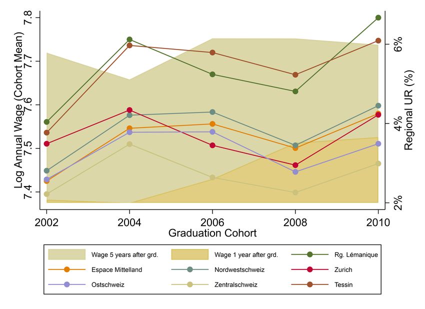
[Insert Figure 1 about here]
Figure 1 plots the mean log wages by cohort versus the regional unemployment rate. From
this Figure it becomes evident that while wages one year after graduation increased throughout
the observation period, the respective cohorts’ wages five years after graduation remained relat-
ively stable. Second, Figure 1 reveals that throughout the covered graduation period (2002-2010)
there was both inter- and intra-regional variation in the unemployment rate. The unemploy-
ment rate reached a peak in 2004 in most regions, decreased thereafter and peaked again in
13
Kahn (2010) and Mansour (2009) work with the hourly wage which they restrict to USD 1–1000 and USD
3–100, respectively.
14
See Altonji et al. (2016), for a similar argumentation.
15
The FSO divides Switzerland into seven regions: Région Lémanique, Espace Mittelland, Nordwestschweiz,
Zurich, Ostschweiz, Zentralschweiz, and Tessin.
16
Unemployment rate calculated according to ILO – see http://www.bfs.admin.ch/bfs/portal/de/index/
themen/03/11/def.html.
17
For instance, Diem and Wolter (2014) also use the unemployment rate in the region, where the individual
attended university as the control variable reflecting economic conditions in their analysis of overeducation among
graduates of Swiss universities.
52010. Between 2004 and 2006, the Tessin surpassed Région Lémanique, which took over the
lead again in 2010 as the region with the highest unemployment rate, while Zentralschweiz
steadily remained the region with the lowest unemployment rate.
3 Empirical Strategy
The aim of this analysis is to identify the effect of the state of the economy in the year of the
individuals’ university graduation on their subsequent labour market outcomes. Therefore, I
start the analysis by regressing an individual’s i wage, yi , on the state of the economy in the
year of her graduation. The state of the economy in the year of the individual’s graduation is
represented by the unemployment rate in the region of her institution of tertiary education and
denoted by U Ri . This specification is defined as follows:
yi = γU Ri + Xi β + ui . (1)
In equation (1), ui denotes an idiosyncratic error term with zero mean and finite variance.
Vector X conveys the fact that an individual’s labour market outcomes may also depend on
various factors that are not related to the state of the economy at the time of her labour market
entry. More specifically, X includes various individual characteristics, such as age, age squared,
gender, nationality, whether an individual has responsibility for children, her canton of origin,18
and dummies indicating whether the individual’s mother and father hold tertiary degrees. The
set of control variables also depicts the details of an individual’s university degree. Namely,
whether the individual holds a degree at the Master’s level,19 her standardised GPA,20 dummies
18
The dummies for the canton of origin serve as a proxy for the individual’s skills, because the cantonal university
eligibility rate (acquired through grammar school graduation, “gymnasiale Maturitätsquote”) varies highly over
the cantons. The rate was between 11.7% for St. Gallen and 32.1% for Basel City in 2015 (FSO, 2015). If one
assumed normally distributed intelligence over the cantons, this would mean that the average university entrant
from St. Gallen is more skilled than the average university entrant from Basel City (for a detailed discussion, see
Ramel, 2015).
19
Since graduates are questioned with respect to the last degree they obtained (compare footnote 7), it is
possible that an individual is represented more than once in the data i.e., first as a Bachelor’s graduate and at a
later point in time as a Master’s graduate. Since the data set is provided by cohorts and without a unique identifier
over all cohorts, there is no possibility to identify these individuals. This problem appears to be negligible for the
rather few cases where an individual has obtained successive degrees in different fields of study. However, there
are certainly individuals in the data who have been surveyed after their Bachelor’s degree and also after having
obtained a Master’s degree. The clustering of the standard errors by individuals is thus not correct in such a
case. I therefore rerun my main regressions under the exclusion of all Bachelor’s graduates. The results remain
qualitatively the same and are therefore not reported here.
20
In order to calculate an individual’s standardised GPA, I first group graduates by field of study, the scale
of their GPA, their institution, year, and type of degree (Bachelor’s or Master’s). Thereafter I standardise the
observed GPA into a variable with mean 0 and variance 1 by subtracting the group’s mean from the individual’s
6for the degree major and the university, and whether an individual has acquired labour market
experience during her studies. The latter is represented by two dummy variables, the first indic-
ating whether an individual had (occasionally or regularly) a job related to her studies and the
second indicating whether she had a job unrelated to her studies. I further enrich the set of con-
trol variables, X, with an individual’s job characteristics that may affect her wage. I control for
working conditions, such as whether the current position requires an academic degree, the type
of employment contract (fixed-term vs. permanent), dummies for the individual’s occupational
status (intern, Ph.D. student/research assistant, employee, or management), dummies for the
individual’s economic area of employment (private, public, non-profit), and the industry sector
of the company the individual is employed in. I also include a dummy for whether the individual
has a side job apart from her main employment. In order to account for possible self-selection
into regions with better employment opportunities, I also include six regional dummies for the
region of employment into my analysis. I control for the state of the economy in the year of the
observation itself by including the regional unemployment rate in the workplace region. I do so,
in order to account for the fact that earning and employment opportunities could be confoun-
ded by the prevailing economic conditions in the moment of the observation itself. Finally, I
also include a linear time trend and its second-degree polynomial into the regression equation.21
Table A.1 in the Appendix provides the definitions and descriptive statistics of the complete set
of variables used in this study.
In order to obtain the maximum of variation, all five cohorts are pooled into one regression,
so equation (1) is estimated using the pooled OLS estimator. Since I include various fixed
effects, the identification relies on intra-individual variation for graduates who are employed in
the same region and sector, attended the same university and pursued the same field of study,
i.e., individuals who follow similar career paths in different years. Equation (1) is estimated
twice. First, only outcomes one year after graduation are considered. Then, only outcomes five
years after graduation are considered.
When observations from both survey periods are pooled in one regression, equation (1) is
observation and dividing this difference by the respective group’s standard deviation.
21
The inclusion of a linear time trend variable only, did not affect my results to a noteworthy extent.
7rewritten in the following way:
yit =γ1 U Ri + γ2 Expit × U Ri + θExpit + X1,i β1 + Expit × X1,i β2
(2)
+X2,it β3 + Expit × X2,it β4 + it .
In equation (2), the moment of the observation, i.e., one or five years after graduation, is
denoted by the index t. Expit is a binary variable with the value 1 if the individual’s potential
experience on the labour market is five years; i.e., this dummy variable indicates that the
observation is from the second survey.22 Expit × U Ri denotes the interaction term of the
regional unemployment rate and potential experience. In this context, γ2 captures how the
effect of the regional unemployment rate at labour market entry on subsequent labour market
outcomes changes between observations; i.e., one and five years after graduation. Furthermore,
the vector X of control variables is now split into a time-invariant component, denoted by X1,i
and a time-variant component, denoted by X2,it . Finally, all control variables are also interacted
with the experience dummy (denoted by Expit × X1,i and Expit × X2,it ). Proceeding in this
way, allows me to utilise the panel structure of the data and to differentiate between the effects
of labour market conditions on wages one year and five years after graduation.
Nevertheless, estimation of equation (2) is likely to suffer from an omitted variable bias
caused by time-invariant and time-varying unobserved individual characteristics. Since the ex-
planatory variable of my analysis is only observed once, i.e., in the year of the individual’s
university graduation, it does not vary over time. In such a setting, the implementation of an
individual fixed effects model is not feasible, because the fixed effects estimator relies on the
within variation. Therefore, I specify a random effects model that relies on both within and
overall variation:
yit =γ1 U Ri + γ2 Expit × U Ri + θExpit + X1,i β1 + Expit × X1,i β2
(3)
+X2,it β3 + Expit × X2,it β4 + ci + vit .
In equation (3), the error term is split into a time-invariant component, ci , and a time-variant
component, vit . However, a major disadvantage of the random effects model is that it relies
on the very strong assumption of mean independence, i.e., E[ci |X1,i , X2,it , U Ri ] = 0, which is
22
Since the actual experience on the labour market could be less than five years for observations five years after
graduation (also due to unfavourable entry conditions), the dummy variable captures potential and not actual
experience (compare Kahn, 2010)
8unlikely to be fulfilled as it implies that the individual heterogeneity cannot be correlated with
any of the regressors. Therefore, I proceed with the so-called Mundlak’s approach and rewrite
equation (3) in the following way:23
yit =γ1 U Ri + γ2 Expit × U Ri + θExpit + X1,i β1 + Expit × X1,i β2
(4)
+X2,it β3 + Expit × X2,it β4 + X2,i λ + µi + vit .
In equation (4), the time-invariant component, ci , is split into the time-invariant stochastic error
term µi and X2,i , the person-specific mean values of all time-varying covariates. Mundlak’s
approach relies on the assumption that after controlling for the person-specific mean values,
the remaining error term µi is no longer correlated with X2 . This approach can therefore be
understood as a “compromise” between the fixed effects and the random effects model.
In contrast to several related studies, I include female individuals in my regressions as labour
force participation is comparable for men and women. For instance, for the 2008 graduation
cohort, it is approximately 95% for both female and male university graduates with a Master’s
degree in both surveys, i.e., one and five years after graduation (Gfeller and Weiss, 2015).
Nevertheless, I also present regression results from separate estimations in Section 5.2.
The main analysis focuses on university graduates, since UAS graduates are often not la-
bour market entrants per se, because these institutions’ entry regulations frequently require a
vocational degree in a field related to the aimed final degree. Furthermore, the degree is often
pursued on an extra-occupational basis. However, in order to account for possible heterogeneity
with respect to skills, job training provided by UAS institutions, pre-degree labour market ex-
perience, and career goals, I run an analysis similar to my main analysis for UAS graduates in
Section 5.2.
Finally, Ph.D.-level graduates are excluded from the main analysis, because the GPA is not
surveyed for this group in the 2008 and 2010 cohorts. However, I run a robustness check, where
these individuals are included for the sake of dropping the GPA from the set of control variables
(see Section 5.1).
23
This approach was originally proposed by Mundlak (1978) and is discussed, for example, in Greene (2008).
94 Results
4.1 Wages and the State of the Economy at Graduation
The results of the regression analyses on the relationship between the regional unemployment
rate and the wages of graduates of Swiss universities are displayed in Table 1. The results for
the regressions of an individual’s wages one year and five years after graduation on the regional
unemployment rate according to equation (1) are displayed in columns (1) and (2), respectively.
The combination of these two regressions according to equation (2) is displayed in column (3).
In this column, the pooled wage is regressed on the regional unemployment rate, the individual’s
potential labour market experience, the interaction term of these two variables, and the vector
X of covariates.
[Insert Table 1 about here]
In all these models, all estimated coefficients are negative and statistically highly signific-
ant. Since the pooled regression (column (3)) is a combination of the two separate regressions,
the initial effect of the regional unemployment rate on log wages corresponds to the result in
column (1), while the post-estimation fitted effect for outcomes five years after an individual’s
graduation, which is the sum of the initial effect and the interaction term, corresponds to the
result in column (2). There appears to be a relatively large (-0.022) and statistically significant
effect for the estimate referring to an individual’s wage one year after her graduation, meaning
that a one-percentage-point increase in the regional unemployment rate in the graduation year
translates into a wage loss of approximately 2.2%.24 According to the OLS specifications, the
effect halves five years after graduation. Thus, there is evidence for a small, but statistically
significant effect of adverse labour market conditions on wages five years after an individual’s
graduation. It means that for university graduates a one-percentage-point increase in the re-
gional unemployment rate in their graduation year translates into a wage loss of approximately
1% five years later. Keeping in mind that my specification accounts for university, field of study,
and region of employment fixed effects, this is, nevertheless, a substantial effect. Finally, the size
of the interaction term between the regional unemployment rate and an individual’s potential
24
Since the dependent variable is log-transformed, a one-percentage-point increase in the explanatory variable
corresponds to a bγ -log-points increase in the dependent variable. The transformation into a percentage value is
γ
calculated as follows: (eb − 1) × 100. However, for small values of b
γ , this transformation can be approximated by
≈bγ × 100. In the following, this is assumed, when interpreting the regression coefficients.
10experience is 0.012, which means that individuals reduce their initial wage gap by approximately
1.2% in the four years following the initial wage observation.
Since the Breusch Pagan LM test for positive variance of the random effects rejects the null
hypothesis of no random effects, results from a random effects regression according to equation
(3) are presented in column (4). Furthermore, I run a F-test for the joint significance of the
averages of all time-variant person-specific variables. The null hypothesis of all averages being
zero is rejected. My preferred specification is therefore a regression that applies Mundlak’s
approach according to equation (4). The results of this regression are displayed in column (5).
However, neither step of correction for potential unobserved individual heterogeneity produces
coefficients that visibly differ from the OLS results, i.e., compared to the OLS specification,
results only differ at the third decimal place. This potentially suggests that controlling for the
observables sufficiently eliminated individual heterogeneity.
The presence of a statistically significant effect of the regional unemployment rate on wages
one year after graduation suggests that even without substantial recessions labour market fluc-
tuations affect wages, nevertheless, the size of the effect on graduates’ wages one year after
their labour market entry is substantially smaller than it is for the United States and Norway,
respectively, as found in Kahn (2010) and Liu et al. (2016). Both studies, however, cover more
volatile periods.
4.2 Self-Selected Timing of Graduation and Adjustment on the Margins?
Several related studies (e.g., Kahn, 2010; Oreopoulos et al., 2012) discuss the possibility of biased
results.25 A bias occurs, if, for instance, individuals time their graduation in accordance with
the state of the economy; i.e., they avoid entering the labour market when the economy is weak.
I therefore analyse, whether potential self-selection issues may have biased my results.
[Insert Table 2 about here]
The associated results are displayed in Table 2.26 First, I run a test for possible self-selection
with respect to the timing of graduation by regressing the gap between the actual and the
expected graduation year on the regional unemployment rate in the year of an individual’s
25
While Kahn’s (2010) results substantially increase after instrumenting the regional unemployment rate, Or-
eopoulos et al. (2012) dismiss their IV specification in favour of the more efficient OLS regression.
26
All these results are conducted on a cross-sectional sample and do not apply econometric techniques that fully
tackle endogeneity. Therefore, these results should be considered as associations without the claim of indicating
causal effects.
11graduation (column (1)). However, I do not find any statistically significant relationship between
this gap and the regional unemployment rate.27
Related to the issue of self-selection in timing is the question of whether the more skilled indi-
viduals are more willing to enter the labour market, so that the previously obtained results may
be biased downwards; i.e., if the more skilled are the only ones who do not shy away from facing
adverse economic conditions, then their outcomes should be better than the potential outcomes
of the average graduates.28 I therefore check, whether particularly capable individuals are the
ones not shying away from graduating in less favourable times and regress the individuals’ final
GPA on the regional unemployment rate (column (2)). I also check whether the probability of
conducting a Ph.D. increases with the regional unemployment rate (column (3)), i.e., individuals
avoid labour market entry by pursuing further education (see, Kahn, 2010). However, again, I
do not find any statistically significant association for both outcomes.
Finally, in line with Kahn (2010), I also analyse the probability of non-employment and
the extent of underemployment by regressing a dummy for whether an individual is working
and the individual’s actual working hours in the year following his graduation on the regional
unemployment rate (columns (4) and (5)), respectively. Both the probability of working and the
amount of working hours appear to slightly decrease with higher regional unemployment rates.
Thus, certain individuals appear to adjust on either the extensive or intensive margin to adverse
entry conditions. Both findings suggests that the resulting wage penalty from adverse economic
conditions could have been higher if these individuals had remained in employment or worked
more hours. Since underemployment may negatively affect subsequent career outcomes, such
as promotion opportunities, this would also contribute to explaining, why wages are negatively
affected by entry conditions even after adjusting them for working hours. This finding is also
in line with Altonji et al. (2016), who identify the lower incidence of full-time employment as
the major driver behind negative outcomes in the post “Great Recession” period in the United
States.
27
I also implemented an IV specification, where I instrumented the regional unemployment rate in the year of
an individual’s graduation with the regional unemployment rate in the expected year of graduation (an approach
similar to, for instance, Kahn, 2010, Mansour, 2009 or Oreopoulos et al., 2012). The results remained qualitatively
similar to the main results with the exception that I observed a complete catch-up after five years in the IV
specification. In the OLS specification, which utilised the same sample as the IV specification, the effect after five
years was reduced to 0.8% and remained statistically significant at the 5% level. Since the C-test for endogeneity
of the main regressor was rejected at the 1% level for the specification which referred to wages one year after
graduation and the sample was reduced by approximately 6,000 observations, I restrained from further following
this approach.
28
Mansour (2009) suggests that the observed scarring effect is usually underestimated because the more skilled
graduates are rather the ones not shying away from entering the labour market in a recession.
124.3 Channels of Catch-up
According to the main results, the persistence of the negative effect of graduating under adverse
conditions is considerably weaker than, for instance, in Kahn (2010) or Liu et al. (2016). In my
specifications, the observed effect almost fades out after five years, which lends some support to
search theory, according to which graduates manage to correct an initially adverse labour market
outcome and catch up with their peers from other, i.e., “luckier”, cohorts. Thus, in order to
contribute to a better comprehension of the underlying channels of the observed catch-up, I
enhance my analysis by regressing further dependent variables on the regional unemployment
rate. In this context, Oreopoulos et al. (2012) suggest that job mobility is a substantial factor
(which is in line with search theory), while Kahn (2010) finds that individuals with initial
wage penalties partly catch-up by working more hours. I therefore, first, analyse how many
job stations an individual has had in the first five years of his career, in order to account for
job mobility. In line with the theoretical argumentation, one would assume that an initial bad
assignment (for instance, caused by an adverse economic situation and consequently fewer jobs
to chose from) should result in subsequent job mobility once the economic conditions improve.
Second, I examine the tenure with the fist job since graduation. In line with the job mobility
hypothesis, it should be lower for individuals who entered the labour market in less favourable
conditions.29 Finally, I verify as to whether individuals who entered in suboptimal conditions
work longer hours in the subsequent years, in order to catch-up potential underemployment,
which arose in the first years.
[Insert Table 3 about here]
Table 3 displays the results of these supplementary regressions.30 Column (1) displays the
estimated incidence rate ratios of the Negative Binomial-ML regression on the relationship
between the regional unemployment rate and the total number of jobs that an individuals has had
in the first five years since his graduation.31 I find a statistically significant positive association
for the total number of jobs that an individuals has had and the regional unemployment rate
29
Kahn (2010) also finds a negative effect of state level entry conditions on tenure in the short run. However,
on the national level she finds that the tenure increases in the long run and interprets this as a hint of lower job
mobility, which may be responsible for potentially slower wage growth of individuals who graduated in recessions.
30
As in the previous Section, all results should be only interpreted as associations and not causal effects (compare
footnote 26).
31
Please note that the number of observations in this regression is lower than in the main specification, since
the section on the employment biography in the first five years since graduation was (i) surveyed five years after
graduation and (ii) contains over-proportionally many missing values.
13prevailing at the moment of his labour market entry, although the effect’s size of approximately
2.7% is relatively small given that the average university graduate has had 2,5 jobs in the first
five years since his graduation (compare Table A.1 in the Appendix). Nevertheless, this finding
provides an indication of job mobility and appears to support the idea that if an initial job match
is suboptimal, individuals move on, in order to improve their career paths, which lends support
to job search theory and the idea of a catch-up. Next, column (2) displays results from a Poisson-
ML regression for the tenure with the first job since graduation.32 In this case, an incidence
rate ratio below one indicates that individuals, who faced higher regional unemployment rates
in the year of their graduation, remained for a shorter period with their first employers than
their peers. This finding lends further support to a potential catch-up via job mobility, but also
indicates that the initial job may have been a suboptimal match. These findings support the
results of, for instance, Oreopoulos et al. (2012) or Bachmann et al. (2010), who suggest that
job mobility explains the declining gap between luckier and less lucky entry cohorts.
Finally, column (3) displays results from the OLS regression of the individuals’ weekly work-
ing hours five years after graduation on the regional unemployment rate in the year of graduation.
In line with Kahn (2010), I find that individuals who experienced suboptimal conditions when
graduating report to work more hours five years later, which at least partly explains the catch-up
in the wage gap.
5 Heterogeneity and Sensitivity Analysis
In this section, I aim at checking the robustness and heterogeneity of the results obtained in the
previous section. In Section 5.1, I check the sensitivity of my main results by running various
robustness checks. Next, in Section 5.2, I analyse the heterogeneity of my main results with
respect to the individuals’ gender, their level of employment (full- or part-time employment)
and the type of their tertiary institution.
5.1 Robustness Checks
[Insert Table 4 about here]
Table 4 presents the results of various robustness checks. In the main analysis, I omitted
32
The likelihood-ratio test for alpha (the over-dispersion parameter) being zero cannot be rejected, therefore,
in this case, the Poisson model appears appropriate as compared to a Negative Binomial model.
14individuals who obtained a Ph.D. as their highest university degree, since for this group the
overall GPA was not surveyed for the 2008 and 2010 cohorts. Although the GPA is an important
confounding variable as it serves as proxy for an individual’s skills, I repeat the main specification
under the exclusion of this variable for the sake of integrating individuals who hold a Ph.D. It
should be noted, however, that this specification still includes a proxy for skills as I account for an
individuals canton of origin (compare footnote 18 in Section 3). The results of this specification
are reported in column (1). The results remain qualitatively the same, although the estimated
coefficient for the initial wage penalty is slightly lower than in the main regression. This could
be explained by both the inclusion and thus dilution of the sample by a group of highly skilled
individuals and the insufficient correction for the confounding variable GPA.
The main specification did not allow me to include graduation region fixed effects, since these
are highly overlapping with the university fixed effects. While I expect very similar results,
because most Swiss greater regions have only one university, it is worthwhile to make this
substitution, in order to account for regional trends. The associated results are presented in
column (2) and there appears to be literally no difference to the main results. Since those few
institutions that are located in the same region are usually of very distinct orientation in terms
of the offered fields of study,33 I prefer to include institution fixed effects over graduation region
fixed effects.
Finally, I present findings, from uncensored wage observations. That is, I restrain from
removing outliers. The associated results are displayed in column (3) and deviate from the
main findings in that I do not observe a statistically significant catch-up effect after five years.
However, as said, this specification included outliers in wage observations, which may potentially
strongly bias the linear regression. I therefore rely on my main approach of censoring extreme
wage outliers, which is in line with the related literature (e.g., Kahn, 2010; Mansour, 2009).
5.2 Heterogeneity Analysis
5.2.1 Entry Conditions and Wages by Gender and Part-Time Status
Despite the very high labour force participation among female graduates of Swiss universities,
the share of female part-time workers is higher than the share of male part-time workers. In
33
For instance, the University of Zurich and the Federal Institute of Technology are located in Zurich. The
latter has a very strong focus on natural sciences and engineering, while the first offers all regular fields of study
covered by universities.
15the analysed sample, the respective shares for women and men are on average, i.e., over all
graduation cohorts, approximately 39% and 25% one year after graduation, and 44% and 23%
four years later. Yet, the consequences of part-time employment include, for example, limited
investment in human capital and thus less steep wage profiles (e.g., Hirsch, 2005). Moreover,
Anderson et al. (2002) suggest that career disruptions for highly skilled women may dampen
human capital accumulation and thus result in lower mid- and long-term wages.34,35 Therefore,
I rerun the main regressions, split by gender and the individuals’ part-time status, i.e., whether
they are employed in full-time or part-time.
[Insert Table 5 about here]
The results from these regressions are presented in Table 5.36 The inspection of columns (1)
and (2), which refer to men and women, respectively, reveals that the direction of the estimated
coefficients is in line with the main estimates. In both regressions, the estimated coefficient with
respect to wages one year after graduation is negative and statistically significant. However, the
coefficients lie below the main estimates for male graduates and above the main estimates for
female graduates. The effect for male graduates halves, while the effect for female graduates
increases by more than 50% as compared to the main results. In precise terms, this means
that a one-percentage-point increase in the regional unemployment rate in the year of a male
university graduate’s labour market entry translates into a wage loss of approximately 1%, while
the corresponding value for a female university graduate is 3.6%. Four years later, for both sexes
a wage penalty of approximately 1% remains, albeit, at lower levels of statistical significance
than in the main analysis.
According to the results of the gender-specific regressions, the adverse effects of unfavourable
entry conditions on wages appear to be stronger for women than for men. Since women are more
frequently employed in part-time, I proceed by examining whether this disparity is caused by
part-timers.37 These results can be found in columns (3) and (4), which refer to full- and
34
Anderson et al.’s (2002) study refers to career disruptions because of children.
35
Also, recent evidence by Hershbein (2012) suggests that women are less likely to be in the labour force in the
first years following high school graduation, when facing adverse entry conditions.
36
I define part-time employees as individuals who report to work less than 40 hours per week, since regular
Swiss full-time employment contracts usually specify 42 working hours per week with some exceptions specifying
40 hours per week. The part-time sample refers to employees who were employed in part-time in both observation
periods. Relaxing this restriction to individuals who were part-time employees in the first observation period
and either part- or full-time employees in the second observation period does not qualitatively affect the results.
However, the effect of adverse entry conditions five years after graduation declines in comparison to the main
part-time sample.
37
van den Berge and Brouwers (2017) conduct a similar heterogeneity analysis with respect to gender for the
16part-time employees, respectively. As suspected, there is an inherent difference between the
effects of adverse entry conditions for full- and part-timer workers, while the estimated wage
penalty one year after labour market entry for full-timers is roughly 1%, it is over 5% for part-
timers. Also, the effect of adverse entry conditions does not persist for full-time employees, but
remains remarkably large for part-time employees. Thus, it appears that my main results are
largely driven by part-time workers. Since the outcome variable, annual wages, is adjusted by
contractual working hours, this finding suggests that there is an additional penalty for part-time
employment under adverse entry conditions. Yet, it should be kept in mind that according to the
results in Section 4.2, the probability of full-time employment declines under adverse economic
conditions, i.e., these results do not permit to disentangle whether the observed increasing
penalty through part-time employment is inter alia driven by the fact that some of the part-
timers are involuntary in such arrangements.38 Thus, their part-time status may at least partly
reflect sub-optimal employer-employee matches, which was previously found to be one of the
main drivers for the wage penalty of adverse labour market entry conditions (see e.g., Liu et al.,
2016).
As it is not clear yet, whether the more prevalent part-time employment among women is
solely responsible for the difference observed between men and women, I additionally present
the results for a sample of full-time employees split by gender in columns (5) and (6). I find that
women who were employed in full-time in both periods catch-up with luckier peers five years
later, yet, the initial wage gap due to adverse labour market entry conditions still appears to
be larger for women than for men. Moreover, for men who were employed in full-time in both
observation periods the scarring effects of adverse entry conditions completely disappear. Thus,
after decomposing the sample, an unexplainable penalty of adverse entry conditions for female
university graduates remains.
Previously job mobility has been suggested as a channel for potential catch-up. I therefore
hypothesise that full-time employees are able to successfully improve their career trajectories
because of higher job mobility.39 In order to verify this assumption, I present again results from
Dutch case. They also attribute the larger negative impacts of entry conditions for women to potential part-time
employment, however, they do not further progress into investigating these heterogeneities.
38
In a specification, which is not presented here, I run an according regression for individuals who were employed
in part-time in the year following their university graduation and in full-time four years later. For these individuals,
the immediate wage penalty is approximately 4%, while the effect vanishes four years later. However, this
specification relies on less than 3,000 observations, so its comparison to the main findings remains questionable.
39
Loprest (1992) suggests that even for full-time employees, wage growth in the first years after labour market
entry is higher for men than for women. Though in her analysis this is not attributed to a higher job mobility
among men per se, but to a higher wage increase associated with job changes for men than for women.
17the specifications discussed in Section 4.3 split by part-time status in Table 6.
[Insert Table 6 about here]
The results presented in Table 6 reveal that indeed job mobility associated with the economic
conditions at labour market entry is significantly lower for part-time than for full-time workers.
This finding hints at the possibility that an individual initially employed in part-time experiences
difficulties in changing his job, for instance, because human capital accumulation on a part-time
job is slower than for comparable full-time employees.40
In total, the results of this heterogeneity analysis indicate that the penalty for disadvantaged
or possibly discriminated groups increases with unfavourable economic conditions.
5.2.2 Entry Conditions and Wages for Graduates of Universities of Applied Sci-
ences
I excluded graduates of UAS from my main analysis, because these graduates differ substantially
in several key characteristics. Therefore, in order to account for possible heterogeneity between
university and UAS graduates, I repeat my main analysis for UAS graduates.
[Insert Table 7 about here]
Table 7 presents the results of wage estimation for UAS graduates. These results exhibit
the same direction as those for university graduates, but differ in that the estimated coefficients
for the initial effect are smaller for UAS graduates than for university graduates. For UAS
graduates, an increase in the regional unemployment rate by one-percentage-point results in
a wage loss of approximately 1.3% one year after their graduation. A possible explanation
for this divergence has already been briefly mentioned in Section 3: Usually UAS graduates
are not labour market entrants per se and often follow their degree on an extra-occupational
basis. Hence, the mechanisms of wage bargaining at work for UAS graduates may not be
the same as for university graduates. In specific, UAS graduates are often professionals who
have completed a vocational training in a field related to their subsequent studies and have
also acquired work experience before following tertiary education. Therefore, on re-entering
the labour market after degree completion they often possess work experience, which is not
40
Table A.2 in the Appendix presents the same heterogeneity analysis by gender. Again, it appears that men
exhibit a higher level of job mobility than women.
18You can also read