UAV: Trajectory Generation and Simulation - Thesis Substitute Project Neha Bhushan - UTA
←
→
Page content transcription
If your browser does not render page correctly, please read the page content below
UTA Research Institute
                           Professor Dr. Frank Lewis

       Thesis Substitute Project

UAV: Trajectory Generation and
          Simulation

              Neha Bhushan

    Date of hand in: May, 2019
        Supervisor: Dr. Frank Lewis
                     Patrik Kolaric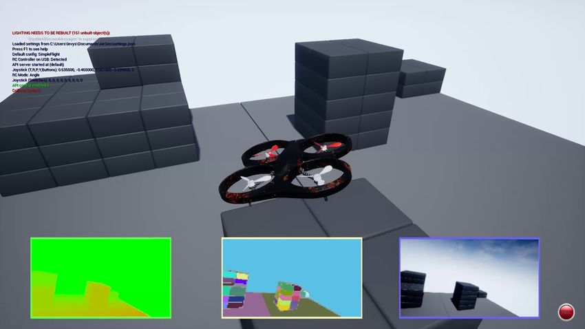
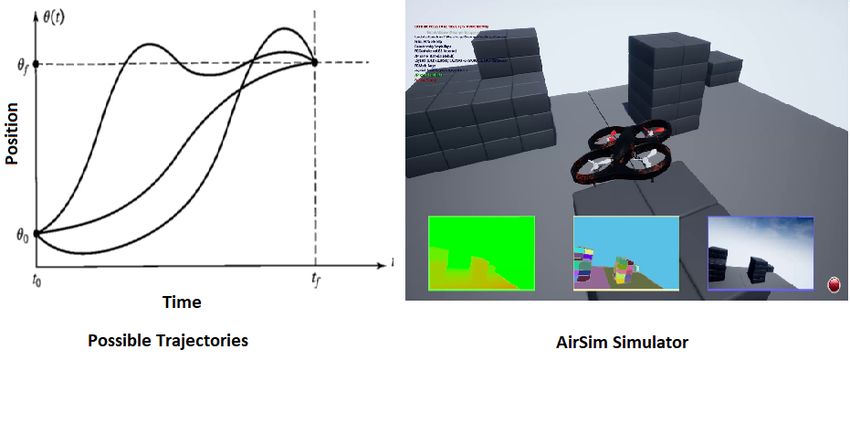
ii
Abstract

Abstract

Unmanned Aerial Vehicles (UAVs) have gained mass popularity in fields such as Defense,
Agriculture, Sport and Photography etc. Their wide adoption in such research projects have
opened new horizons for opportunities. However, UAVs operate in a rather dynamic environ-
ment since various factors such as airspeed, temperature, pressure, turbulence etc. are capable
of hampering the flight operation. There is a need for rather robust trajectory generation al-
gorithm and system such that it provides an easy user interface to specify the path of UAV
through space, alongside making the UAV capable enough to maneuver itself from the initial
to final position. This project focuses on two aspects of UAV control, the first part focuses
on trajectory generation using various mathematically modeled techniques for the position,
velocity and acceleration expressed as a function of time. Their comparison is done based on
the constraint-based optimization techniques followed by some discussions. The second part
focuses on UAV simulators and lays out the foundations and requirements for them, followed
by some proposed simulators and their comparison, which could be used not only for flight
control simulation, but also have potential to integrate Reinforcement Learning techniques
for Autonomous flight control and Autopilot systems. Finally, in-depth analysis of AirSim
simulator is carried out along with its environment setup process which may be used as an
Interfacing, Installation and set-up documentation for future work.

Title page image: First image demonstrates Potential Trajectory functions. Second image is
a sample simulated AirSim Blocks environment.

iii
                          Acknowledgement

I, Neha Bhushan, Masters Student in Electrical Engineering at the University of Texas, Arling-
ton would like to extend my deepest appreciation and acknowledgement to Dr. Frank Lewis
and Patrik Kolaric associated with the University of Texas Arlington and UTA Research In-
stitute. This project would not have been possible to accomplish without their continuous
support and feedback. Special appreciation to Vatsal Joshi and Mohit Kalra who provided
assistance with work stations and IT infrastructure. Last but not the least, many thanks to
my University for all the resources and its Graduate advisors for guiding me throughout my
course curriculum and thesis project.
Contents

1. Introduction                                                                                                                                    1
   1.1. UAV: Overview . . . . . . . . . . . . . . . . . . . . . . . . . . . . . . . . .                                                            1
   1.2. Dynamic Environment . . . . . . . . . . . . . . . . . . . . . . . . . . . . .                                                              1
   1.3. Trajectory . . . . . . . . . . . . . . . . . . . . . . . . . . . . . . . . . . . .                                                         1

2. Motivation                                                                                                                                      3
   2.1. Control Strategies . . . . . . . . . . .               .   .   .   .   .   .   .   .   .   .   .   .   .   .   .   .   .   .   .   .   .   3
   2.2. Application Areas . . . . . . . . . . .                .   .   .   .   .   .   .   .   .   .   .   .   .   .   .   .   .   .   .   .   .   3
        2.2.1. Research Platform . . . . . .                   .   .   .   .   .   .   .   .   .   .   .   .   .   .   .   .   .   .   .   .   .   3
        2.2.2. Military and Law Enforcement                    .   .   .   .   .   .   .   .   .   .   .   .   .   .   .   .   .   .   .   .   .   3
        2.2.3. Photography . . . . . . . . .                   .   .   .   .   .   .   .   .   .   .   .   .   .   .   .   .   .   .   .   .   .   4
        2.2.4. Drone-Delivery . . . . . . . .                  .   .   .   .   .   .   .   .   .   .   .   .   .   .   .   .   .   .   .   .   .   4
        2.2.5. Industrial Site Inspection . . .                .   .   .   .   .   .   .   .   .   .   .   .   .   .   .   .   .   .   .   .   .   4
        2.2.6. Agriculture and Forests . . . .                 .   .   .   .   .   .   .   .   .   .   .   .   .   .   .   .   .   .   .   .   .   4
        2.2.7. Archeology . . . . . . . . . .                  .   .   .   .   .   .   .   .   .   .   .   .   .   .   .   .   .   .   .   .   .   5
        2.2.8. Weather and Storm Analysis .                    .   .   .   .   .   .   .   .   .   .   .   .   .   .   .   .   .   .   .   .   .   5
        2.2.9. Emergency Response . . . . .                    .   .   .   .   .   .   .   .   .   .   .   .   .   .   .   .   .   .   .   .   .   5
   2.3. Mechanical Structure . . . . . . . . .                 .   .   .   .   .   .   .   .   .   .   .   .   .   .   .   .   .   .   .   .   .   5
   2.4. Flight Dynamics . . . . . . . . . . . .                .   .   .   .   .   .   .   .   .   .   .   .   .   .   .   .   .   .   .   .   .   6

3. Trajectory Generation                                                                                                                            8
   3.1. Overview . . . . . . . . . . . . . . . .                   .   .   .   .   .   .   .   .   .   .   .   .   .   .   .   .   .   .   .   .    8
   3.2. Proposed Methods . . . . . . . . . . .                     .   .   .   .   .   .   .   .   .   .   .   .   .   .   .   .   .   .   .   .    9
        3.2.1. Cubic Polynomials . . . . . . .                     .   .   .   .   .   .   .   .   .   .   .   .   .   .   .   .   .   .   .   .    9
        3.2.2. Linear blend . . . . . . . . . .                    .   .   .   .   .   .   .   .   .   .   .   .   .   .   .   .   .   .   .   .   10
   3.3. Trigonometric Functions . . . . . . . .                    .   .   .   .   .   .   .   .   .   .   .   .   .   .   .   .   .   .   .   .   10
        3.3.1. Arc Tangent Function . . . . .                      .   .   .   .   .   .   .   .   .   .   .   .   .   .   .   .   .   .   .   .   10
        3.3.2. Sine, Cos Function . . . . . . .                    .   .   .   .   .   .   .   .   .   .   .   .   .   .   .   .   .   .   .   .   12
   3.4. Implementation of Trajectory Generator                     .   .   .   .   .   .   .   .   .   .   .   .   .   .   .   .   .   .   .   .   12

4. Simulator                                                                                                                                       14
   4.1. Introduction . . . . . . . .   .   .   .   .   .   .   .   .   .   .   .   .   .   .   .   .   .   .   .   .   .   .   .   .   .   .   .   14
   4.2. UAV Systems . . . . . . .      .   .   .   .   .   .   .   .   .   .   .   .   .   .   .   .   .   .   .   .   .   .   .   .   .   .   .   14
   4.3. Simulator Requirements .       .   .   .   .   .   .   .   .   .   .   .   .   .   .   .   .   .   .   .   .   .   .   .   .   .   .   .   15
        4.3.1. Physical Modelling      .   .   .   .   .   .   .   .   .   .   .   .   .   .   .   .   .   .   .   .   .   .   .   .   .   .   .   15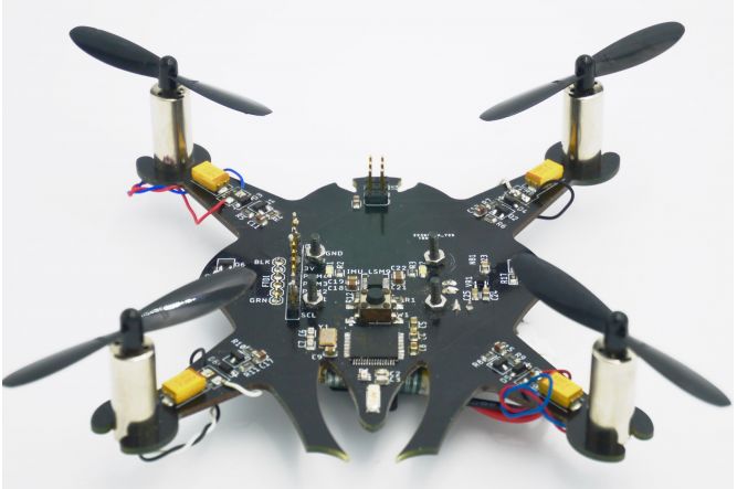
4.3.2.   Environment . . . . . .                  .   .   .   .   .   .   .   .   .   .   .   .   .   .   .   .   .   .   .   .   .   .   .   .   15
         4.3.3.   Reinforcement Learning                   .   .   .   .   .   .   .   .   .   .   .   .   .   .   .   .   .   .   .   .   .   .   .   .   16
         4.3.4.   Long Term Support . . .                  .   .   .   .   .   .   .   .   .   .   .   .   .   .   .   .   .   .   .   .   .   .   .   .   17
         4.3.5.   Interface . . . . . . . .                .   .   .   .   .   .   .   .   .   .   .   .   .   .   .   .   .   .   .   .   .   .   .   .   17

5. Choice of Simulators                                                                                                                                    19
   5.1. Gazebo . . . . . .     .   .   .   .   .   .   .   .   .   .   .   .   .   .   .   .   .   .   .   .   .   .   .   .   .   .   .   .   .   .   .   19
   5.2. Hector Quadrotor .     .   .   .   .   .   .   .   .   .   .   .   .   .   .   .   .   .   .   .   .   .   .   .   .   .   .   .   .   .   .   .   19
   5.3. TUM Simulator . .      .   .   .   .   .   .   .   .   .   .   .   .   .   .   .   .   .   .   .   .   .   .   .   .   .   .   .   .   .   .   .   20
   5.4. GymFC . . . . . .      .   .   .   .   .   .   .   .   .   .   .   .   .   .   .   .   .   .   .   .   .   .   .   .   .   .   .   .   .   .   .   20
   5.5. AirSim . . . . . . .   .   .   .   .   .   .   .   .   .   .   .   .   .   .   .   .   .   .   .   .   .   .   .   .   .   .   .   .   .   .   .   21

6. AirSim                                                                                                                                                  23
   6.1. Architecture . . . . . . . .           .   .   .   .   .   .   .   .   .   .   .   .   .   .   .   .   .   .   .   .   .   .   .   .   .   .   .   23
   6.2. Mathematical Model . . .               .   .   .   .   .   .   .   .   .   .   .   .   .   .   .   .   .   .   .   .   .   .   .   .   .   .   .   24
        6.2.1. Vehicle Model . .               .   .   .   .   .   .   .   .   .   .   .   .   .   .   .   .   .   .   .   .   .   .   .   .   .   .   .   24
        6.2.2. Gravity . . . . . .             .   .   .   .   .   .   .   .   .   .   .   .   .   .   .   .   .   .   .   .   .   .   .   .   .   .   .   25
        6.2.3. Magnetic Field . .              .   .   .   .   .   .   .   .   .   .   .   .   .   .   .   .   .   .   .   .   .   .   .   .   .   .   .   25
        6.2.4. Accelerations . . .             .   .   .   .   .   .   .   .   .   .   .   .   .   .   .   .   .   .   .   .   .   .   .   .   .   .   .   25
   6.3. Flight Controller . . . . .            .   .   .   .   .   .   .   .   .   .   .   .   .   .   .   .   .   .   .   .   .   .   .   .   .   .   .   26
        6.3.1. Hardware-in-Loop                .   .   .   .   .   .   .   .   .   .   .   .   .   .   .   .   .   .   .   .   .   .   .   .   .   .   .   26
        6.3.2. Software-in-Loop .              .   .   .   .   .   .   .   .   .   .   .   .   .   .   .   .   .   .   .   .   .   .   .   .   .   .   .   26
        6.3.3. simple_flight . . .             .   .   .   .   .   .   .   .   .   .   .   .   .   .   .   .   .   .   .   .   .   .   .   .   .   .   .   26
        6.3.4. PX4 . . . . . . . .             .   .   .   .   .   .   .   .   .   .   .   .   .   .   .   .   .   .   .   .   .   .   .   .   .   .   .   27

7. Conclusion                                                                                                                                              30

A. (Appendix) AirSim: Documentation and Installation Instructions                                                                                          31
   A.1. Code Structure . . . . . . . . . . . . . . . . . . . . . . . . . . . . .                                                           .   .   .   .   31
        A.1.1. AirLib . . . . . . . . . . . . . . . . . . . . . . . . . . . . . .                                                          .   .   .   .   31
        A.1.2. Unreal/Plugins/AirSim . . . . . . . . . . . . . . . . . . . . .                                                             .   .   .   .   31
        A.1.3. MavLinkCom . . . . . . . . . . . . . . . . . . . . . . . . . .                                                              .   .   .   .   32
        A.1.4. Unreal Framework . . . . . . . . . . . . . . . . . . . . . . .                                                              .   .   .   .   32
   A.2. System Requirements . . . . . . . . . . . . . . . . . . . . . . . . . .                                                            .   .   .   .   32
        A.2.1. Hardware Requirements . . . . . . . . . . . . . . . . . . . .                                                               .   .   .   .   32
        A.2.2. Software Requirements . . . . . . . . . . . . . . . . . . . . .                                                             .   .   .   .   32
   A.3. Installation Instructions . . . . . . . . . . . . . . . . . . . . . . . . .                                                        .   .   .   .   33
        A.3.1. Option 1: Download pre-compiled Binaries . . . . . . . . . .                                                                .   .   .   .   33
        A.3.2. Option 2: Build AirSim . . . . . . . . . . . . . . . . . . . .                                                              .   .   .   .   33
   A.4. Setup Instructions . . . . . . . . . . . . . . . . . . . . . . . . . . . .                                                         .   .   .   .   33
        A.4.1. Unreal Environment . . . . . . . . . . . . . . . . . . . . . .                                                              .   .   .   .   33
        A.4.2. AirSim Environment: Blocks . . . . . . . . . . . . . . . . . .                                                              .   .   .   .   34
   A.5. Programmatic Control . . . . . . . . . . . . . . . . . . . . . . . . .                                                             .   .   .   .   34
   A.6. Application Programming Interfaces (APIs) . . . . . . . . . . . . . .                                                              .   .   .   .   34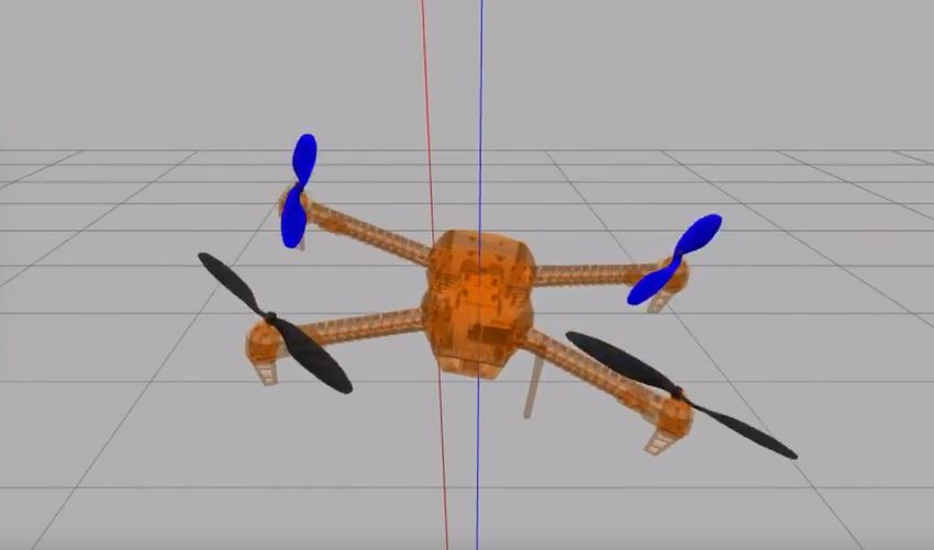
A.7. APIs for Multimotor . . . . . . . . . . . . . . . . . . .     .   .   .   .   .   .   .   .   .   .   .   35
  A.8. APIs Explained . . . . . . . . . . . . . . . . . . . . . .    .   .   .   .   .   .   .   .   .   .   .   36
       A.8.1. getMultirotorState . . . . . . . . . . . . . . . .     .   .   .   .   .   .   .   .   .   .   .   36
       A.8.2. Async methods, duration and max_wait_seconds           .   .   .   .   .   .   .   .   .   .   .   36
       A.8.3. Drivetrain . . . . . . . . . . . . . . . . . . . . .   .   .   .   .   .   .   .   .   .   .   .   37
       A.8.4. yaw_mode . . . . . . . . . . . . . . . . . . . .       .   .   .   .   .   .   .   .   .   .   .   37
       A.8.5. lookahead and adaptive_lookahead . . . . . . .         .   .   .   .   .   .   .   .   .   .   .   37

Bibliography                                                                                                     43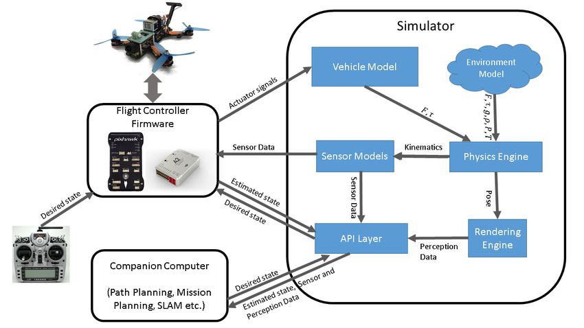
1

1. Introduction

1.1. UAV: Overview
Unmanned Aerial Vehicles (UAVs) have been gaining momentum in their popularity in wide
application fields such as surveillance and monitoring, aerial imaging, cargo delivery, photog-
raphy etc [23] [9]. Being Aerial, UAVs are independent of terrain unlike Unmanned Ground
Vehicles (UGVs) where the application use cases might be hindered by unfavorable terrain
contours for which the system might not be designed for. In fact, UAVs can easily fly and
reach inspection points, record surveillance data and transmit the information to the base sta-
tion wirelessly. Being Airborne brings its own set of challenges, limitations. Take aerial traffic
for example, just like vehicles running on the ground, UAVs may collide with each other in
the air especially for densely populated areas where geographically practical use case of UAV
is higher. In residential or commercial places this collision could be disastrous. Furthermore,
in a modern city of the present, we have many high-rise buildings and skyscrapers acting as
objects of hinderance leaving limited room for maneuverability.

1.2. Dynamic Environment
UAVs operate in a rather dynamic environment; another type of challenge is the physical char-
acteristics of Airflow in the environment. Factors such as airspeed, air pressure, temperature,
turbulence etc. [17] have the potential to disrupt flight operation and prove fatal for the UAV.
Among several open problems related to UAV, trajectory generation is of immense signifi-
cance which pertains generating a feasible yet optimal or optimally closest flight trajectory in
respect to all limitations and constraints such as but not limited to minimum and maximum
maneuvering radius, minimum and maximum speed, obstacle and terrain collision avoidance
[4].

1.3. Trajectory
Trajectory refers to change in position, velocity, and acceleration of UAV with respect to time
for the motion of a UAV. In this project, trajectory generation deals with describing the desired
motion of UAV in a way that it is easy for user to specify the path of UAV through space rather
than calculating its complicated functions in space and time. For the purpose of this project,
2

it is required to generate trajectory for desired initial position, final position and time to reach
that position and leave it to the system to decide on the exact shape of the path to get there and
calculate the respective the velocity profile.

                      Figure 1.1.: Example of Generated and Actual path

As seen in Fig. 1.1 [7], ], for a typical flight controller, the actual path might differ from the
generated path due to presence of obstacles and non-linear characteristics of the controller. In
case of UAV flight, it is desirable for the motion to be smooth so that the jerks don’t cause the
UAV to have erratic behavior like flip in the middle of flight. For a function to be smooth it is
desired to be continuous and have a continuous first and second derivatives.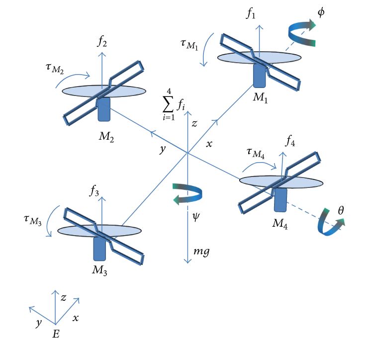
3

2. Motivation
UAVs have become increasingly popular due to their versatile nature and potential to solve
real-life challenges in a wide horizon of industry. Environments which are mostly inaccessible
to other types of aircrafts such as low-altitude flying in urban areas, carrying out tasks where
situation is hazardous for humans prove to be the most generating markets for them. Since
UAVs operate without a human on board pilot, there are mainly two control strategies: Remote
Control or Autonomous Control. [4]

2.1. Control Strategies
In Remote Control, the onboard flight controller receives commands from the base station re-
garding the trajectory, initial final position, and other flight-critical parameters. At the base
station a human pilot flies through the remote controller communicating with Radio Frequency
Link. With recent advances in navigation systems, embedded systems, modern microcon-
troller architectures are getting computationally powerful yet consuming less and less power.
This coupled with optimization techniques and digital vision systems have broadened the de-
gree of reliability and autonomy making modern-day UAVs extremely versatile.

2.2. Application Areas
Some of the potential use cases of UAVs are as follows.

2.2.1. Research Platform
Quadcopters are an extremely useful tool and development platform for University Students
and Researchers to validate various control strategies and Algorithms in a real-life scenario to
study the flight dynamics and impact of environmental factors such as airspeed, temperature,
humidity, turbulence etc. Algorithms relating to flight navigation can also be tested on small
inexpensive platforms before deploying them on expensive hardware.

2.2.2. Military and Law Enforcement
UAVs are used for surveillance by Military and defense organizations wherever needed for
the sake of National Security. These UAVs are generally equipped with Multispectral image
4

sensors, such as RGBD cameras, Infrared based thermal sensing for night-sight vision. Some
UAVs depending on application might also be capable of occlusion motions flow sensors and
motion detectors for critical areas like border crossings and Secured test sites.

2.2.3. Photography
Initially used by professional cinematographers, drones equipped with cameras are gain-
ing mass popularity among millennial travelers for photography and videography. Massive
progress has been made towards portable and foldable quadcopters design with advanced tech-
nology such as Optical Image Stabilization and Object following technology making its way
into commercial photography drones.

2.2.4. Drone-Delivery
Many companies such as Deutsche Post and Amazon prime have been experimenting to at-
tempt home delivery of parcels and couriers using drones. These solutions may ultimately
prove to be revolutionary for the shipping and logistics industry as they solve the problem
of last mile delivery connectivity situation, thereby enabling faster deliveries in downtown
metropolitan areas and among high-rise residential. Moreover some food startups are trying
to utilize drone potential to make deliveries for home-orders which increases the quality of
service since it drastically reduces the time-to-home.

2.2.5. Industrial Site Inspection
This is one particular area that has highly impactful real-life use case for the UAVs. Very often
in or nearby industrial sites, such as chemical plants, Thermal Power plants as well as Nuclear
Plants, site inspection is mandated to ensure safe functionality of these plants. Due to their
sheer size, physically it is not possible for humans to inspect all the aspects of them. Drones
are gaining mass popularity in these use cases. When equipped with multispectral camera
sensors and gas sensors, these can be used for monitoring health of a boiler, reactor or furnace
exhaust. With onboard integrated sensors, they collect valuable data which might be helpful
in detecting or preventing industrial leakage which might be catastrophic.

2.2.6. Agriculture and Forests
There are quite a number of civil applications of UAVs. Recently, many governmental orga-
nizations such as the forest department and municipalities have been using drones for Aerial
3D mapping of a locality along with Aerial surveys for crops, inspection of power lines /
pipelines, counting and analyzing wildfires, detection of illegal hunting, providing medical
support in areas which are otherwise not accessible etc.
5

2.2.7. Archeology
In Latin America, drones have been increasingly replacing the use of small planes, kites and
helium balloons as the latter have proven to be expensive and difficult to operate as compared
to UAVs. Smaller UAVs have been capable to producing 3D models of Peruvian sites instead
of flat-maps in a relatively shorter period of time.

2.2.8. Weather and Storm Analysis
UAVs are especially useful in accessing areas that are hazardous for manned vehicles. Sit-
uations such as hurricanes, tornadoes and cyclones are some of the typical example where
usually manned aircrafts are warned to stay away from. In such cases inexpensive UAVs can
be used for in-depth analysis of such calamities to gather crucial data, which helps in making
plans for emergency response and evacuations if need be. Such systems are equipped with
necessary barometric and temperature sensors which transmit the data wirelessly.

2.2.9. Emergency Response
Even in post-calamity conditions, drones have proven to be extremely effective in search and
rescue operations alongside property damage assessment. Typical payloads include optical
sensors, radars to capture imagery and analyze terrain situation. Similarly, when equipped
with gas sensors, they can be used to analyze the pollutions levels and severity especially for
cities like New Delhi and Beijing with critical pollution levels.

2.3. Mechanical Structure
For a typical quadcopter construction, there are these following components.
   1. Frame
   2. Propellers (fixed pitch or variable pitch)
   3. Electric Motors
   4. Battery
   5. Flight Controller and Electronics
Generally, to obtain optimum performance and simple control system, the motors and pro-
pellers are placed equidistant from each other. To improve the power to weight ratio, exotic
materials such are carbon fibre are used in the chassis and mechanical structure construction
as these offer exceptionally well, strength to weight ratio, thus enabling UAVs to drastically
be lighter. This not only improves the maneuverability but also enhances flight time as battery
could be used more efficiently.
6

                             Figure 2.1.: Quadcopter Design [21]

2.4. Flight Dynamics
Flight dynamics of a UAV are quite complex and explode exponentially as the number of
rotors increase such as for a hexacopter and an octocopter. To break the dynamics down in
simpler forms, it is easier to model and understand for a four-rotor design.
A quadcopter has two pairs of rotors in cross-configuration which are capable of rotating
at different angular velocities (rads/sec) This differential velocities enable the quadcopter to
achieve rotational and translation motion. Detailed dynamics can be found in the words of
Ali et. al [3]. The following equations briefly summarize the dynamics. the total thrust u is
described as [6].

                                     u = f1 + f2 + f3 + f4

where f1 f2 f3 f4 denote the upwards thrust generated by each rotor.

                                     fi = ki ωi2 , i = 1, ..., 4

where ki > 0 is a constant and ω is the angular speed of the respective motor, m is the mass of
the quadcopter and g is the gravitational acceleration.

                                        mẍ = −u sin θ
7
Figure 2.2.: Quadcopter Dynamics [19]
mÿ = u cos θ sin φ
mz̈ = u cos θ cos φ − mg
ψ̈ = τψ
θ̈ = τθ
φ̈ = τφ
τψ τθ τφ denote the control inputs for yaw, pitch and roll respectively.8
3. Trajectory Generation
3.1. Overview
Our functional requirements can be formulated as follows. Since there are n number of pos-
sible permutations and combination for a UAV to travel from initial to the final positions. We
apply constraints of limited time window along-side having jerk-free motion.
Let p(t) denote the position as a function of time. Let p(0),p( f ) denote the initial and final
positions of the UAV respectively. Let the timing constraints for the UAV to reach from initial
to final position be given by t0 and t f respectively. Figure 3.1 shows the possible smooth
function trajectories which might be feasible. Of these, the one with most optimal trajectory
should be used.
Figure 3.1.: Example of Possible smooth trajectories
In making a smooth motion, at least four constraints on p(t) are evident. To derive simpler
equations, the characteristics are considered to be one dimensional rather than the actual 3-
dimensional model for the physical system. Two constraints on the function’s value come
from the selection of initial and final values:
tf =T9
p(0) = P0
p(t f ) = Pf
Additional two constraints are that the velocity function be continuous as the UAV starts and
stops at the final position, which in this case means that the initial and final velocity on UAV
are zero:
ṗ(0) = 0
ṗ(t f ) = 0
3.2. Proposed Methods
Trajectory generation problems in robotics are generally solved using Cubic Polynomials and
Linear function with parabolic blends. The solutions explored are briefly described below:
3.2.1. Cubic Polynomials
p(t) = x0 + x1t + x2t 2 + x3t 3
p(0) = x0 = P0
p(t) = P0 + x1t + x2t 2 + x3t 3
v(0) = ṗ(0) = x1 = 0
v(t) = ṗ(t) = x1 + 2x2t + 3x3t 2
a(0) = v̇(0) = 2x2 = 0
v(t) = ṗ(t) = 2x2 + 6x3t
Using this method accelerations can’t be zero as it will make all the coefficients zero and for
smooth trajectory, these accelerations are desired to be minimized which in turn affects its10
efficiency in term of time to reach goal position. To have the desired trajectory, we will need
higher order polynomials which makes the equation more complex. To follow the constraints,
we will have to solve the trajectory problem for third order derivative i.e. jerk and fourth order
derivative i.e. snap.
3.2.2. Linear blend
In case of linear blend, the motion from the initial to the final position is simply linearly
interpolated as seen in Fig. 3.2. However, if such a trajectory is desired, it would result in
velocity to be discontinuous as the system would demand abrupt changes in infinitesimally
small time from 0 to v f inal in the starting phase and v f inal to 0 in the final phase thereby
resulting in infinite acceleration in both.To create a smooth path with continuous position and
velocity we add parabolic terminators at both these phases as shown in Fig. 3.2. As the
acceleration increases, the length of the blend region becomes shorter and shorter. In the limit,
with infinite acceleration, we are back to the simple linear-interpolation case.
Figure 3.2.: Linear Interpolation with (a) Infinite acceleration (b) Parabolic Blends
Fig. 3.3 (a) shows a case where the value of acceleration is chosen to be quite high. In
such cases, we quickly move from initial to the final position, this results in nearly constant
velocity with noticeable changes only during the beginning and the end phase. For (b) we see
that acceleration is lower as compared to the previous case hence the linear section disappears
and the curve appears parabolic.
3.3. Trigonometric Functions
3.3.1. Arc Tangent Function
Due to uneven acceleration values for linear blend, cubic polynomial seems like a better
choice. Mathematical functions like exponential and trigonometric functions can be used11
Figure 3.3.: Example curves of position, velocity, acceleration in Linear Interpolation (a)
Higher Accleration (b) Lower Acceleration
similarly for trajectory generation as they produce similar results when differentiated. Trans-
formation of these functions and curve fitting methods can be used to produce results for
problem at hand. Trigonometric functions like arctan and cos are best suited for the desired
position curve. I went ahead with testing the arctan function first. Considering the variables,
A, B, C and D for transformation of functions we can start with the equation below.
p = C. arctan(At − B) + D
For the given curve of final position can be defined as:
p = 0.9lim [C. arctan(At − B) + D]
t→∞12
π
p f = 0.9[C. + D]
2
P0 = −C. arctan(B) + D = 0
Considering max velocity A = Vmax C , Solving these equations did not come up with a very
smooth curve as the variables in this equation are not independent.
3.3.2. Sine, Cos Function
The other solution is transforming cos functions and limiting them generated more desirable
curve. The equation used for position, velocity and acceleration as follows
Pf π Pf
p(t) = − cos( .t) +
2 T 2
pf π π
v(t) = . sin( .t)
2 T T
Pf π π π
a(t) = . . cos( .t)
2 T T T
The curves generated for these equations are well suited for smooth trajectories and are hence
preferred.
Figure 3.4.: Position, Velocity, Acceleration curves
3.4. Implementation of Trajectory Generator
Trajectory Generator only generates a path for the UAV from an initial position to the final
position. However during a UAV flight and motion, other aspects such as Hovering, Dynam-
ical Rotor control and actual flight are not directly controlled by the Trajectory Generated.13 When actually using the trajectory generator for desired motion of UAV, the trajectory gener- ator must be triggered at the time of defining path or guiding the UAV from starting position to desired final position and after reaching the final position, a threshold of a small value (eg. 10 cm) must be considered to kill the trajectory generator and override by the hover function to make the UAV stop and hover at the final position.
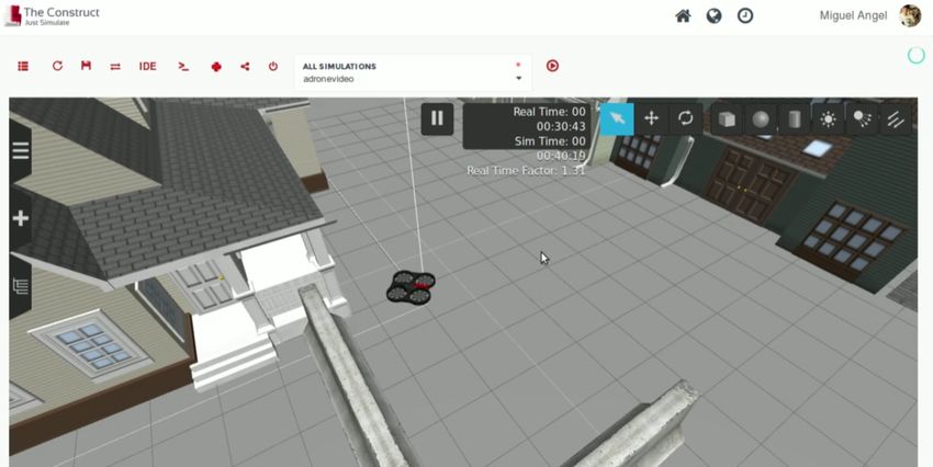
14

4. Simulator

4.1. Introduction
Simulation has always been an integral tool in robotics and is a reliable source to generate
useful data by saving time and cost. Testing of any robotic hardware or software can be done
by simulation by creating number of scenarios and the reaction of robot in these scenarios
for example a hundred of seconds of real-world scenario can be enacted in one second of a
simulation. Moreover, it lets user to study and perform research in complex missions that may
be time-consuming and risky in real-world. Virtually, the mistakes or bugs in simulation cost
nothing as the vehicle can crash multiple times and hence the implementation of a concept can
be debugged by learning through the simulation of the concept in various conditions. In case
of UAVs, developing and testing algorithms in real world can be very expensive and time-
consuming. Moreover, utilizing current research and advancement in machine intelligence
and deep learning requires collection of huge amounts of training and testing of in a variety of
conditions and environments.

4.2. UAV Systems
UAV system simulation is desired to train UAV to control and navigate by its own thereby
having fully autonomous capabilities. The flight simulator is desired to artificially recreate
the UAV flight dynamics and environment in which it flies by simulating aerodynamic model.
This is done by replicating the equations that govern the control of UAV, their reaction to
external factors such as air density, turbulence, wind shear, cloud, precipitation, etc. The
best simulators generally offer a variety of courses, variable weather conditions and realistic
physics to keep it as realistic and practically applicable as possible.
However, simulating the real-world is a big challenge. To operate a UAV in the real-world
without any hurdles it is important to be able to transfer the learning it does in simulation as
the simulation and real-world varies a lot. One of the most difficult components in this aspect
is simulating the detailed physics of the environment [22]. For a UAV simulation system,
physics includes perception, sensing and the dynamics of the system, ground and atmosphere.
Therefore, it is important to develop accurate models of the UAV system dynamics so that
simulated behavior enacts the real-world as accurately as possible.
15

                      Figure 4.1.: Quadcopter Simulation Environment

4.3. Simulator Requirements
For a typical UAV simulator we have the following requirements.
   1. Good physical model that include aerodynamical effects like wind and gravity.
   2. Realistic Environment for better use at time of implementing in real world.
   3. Reinforcement Learning integration.
   4. Long term support and easy to use for other users.
   5. Good interface for system integration and hardware in loop testing.

4.3.1. Physical Modelling
For a typical UAV simulator, the quality of the environment and simulating engine depends on
how well detailed and complex is the physical model. The environment is more real-life like if
it supports the effects of wind gusts, precise gravitational forces, air temperature and pressure.
Since these parameters are beyond the control of the system, modelling them enhances the
robustness of algorithm and system design. Some even more complex parameters such as
aerodynamical effects play a critical role in higher altitude and high-speed maneuvers during
a flight. Having such properties is highly desirable in a simulator.

4.3.2. Environment
For vision-based systems and simulators supporting trajectory generation and path planning.
Detailed modelling of the environment and setting becomes crucial, since the algorithm of
16
the system being tested in the simulated environment might be custom tailored for some cus-
tom and specific scenarios. Typical examples of Environment includes, Hill Side, City Life,
Parks, Indoors. Depending on the use case and application area, some simulators might have
an advantage over the rest. It is highly desirable to have a simulator that supports multiple
environments and has extensions or add-ons, where newly modelled environments could be
easily integrated.
Figure 4.2.: Indoor Simulator Environment [10]
Figure 4.3.: City Simulator Environment [12]
4.3.3. Reinforcement Learning
With the advancement of Machine Learning based algorithms and techniques, simulators have
gained massive popularity. Certain unsupervised learning techniques such as K-means cluster-17
ing and Q-Learning based DQN networks have a massive advantage over supervised learning
techniques in a way that they do not require labelled dataset, i.e. they do not require for each
input label x to have an output label y. This has massive implications in terms of savings
in time and resources as manually labelling dataset is quite expensive and time-consuming.
Rather by utilizing the techniques of reward and penalty, a cost function could be formulated
where, the network can be trained on massive unlabelled data, which learns by optimizing the
cost function by minimizing the penalty and maximizing the reward.
Figure 4.4.: Reinforcement Learning Block Diagram
Such learning frameworks are usually based on Python or R, hence if the simulator is capa-
ble to be interfaced by using certain Application Programming Interfaces (APIs) along with
TensorFlow, Caffee, is an added advantage. When configured correctly, the system could be
initialized by integrating with the simulator and ideally train on infinite amount of simulated
data without the need for manual labelling, thereby truly creating an Artificially Intelligent
system.
4.3.4. Long Term Support
Long Term Support or legacy support is critical from a life-cycle management point of view.
Traditional development of new projects tend to take a few years depending on the complexity
of the underlying system. Meanwhile, if the simulator is discontinued or is not constantly
being updated according to the state-of-the-art standards results in a buggy development envi-
ronments which is not at all desirable. Long-term support also ensures wider adoptability of
a simulator since developers are willing to pay a premium over support, which leads to even
wider adoption and hence creates a positive improvement life-cycle.
4.3.5. Interface
System integration, APIs, IOs and Hardware-in-loop testing is another crucial characteristic
for a simulator. Many a times, after validating the system in a simulated environment, it is
important to verify it in actual hardware setting before a test flight. However, due to high18
degree of uncertainty, there is a high degree of risk associated with actual flight and using
expensive hardware for such tests. Hardware-in-loop is an excellent verification methodology
which ensures that the algorithm performs at par in performance as compared when tested in
a simulated environment. This enables to check the hardware functionality running the actual
algorithm yet in a simulated environment, such that even if certain things go hay-wire, no
damage is done to expensive hardware. Similar extensive hardware interfacing and integration
is desirable since devices supporting various communication protocols could be interfaced.
Figure 4.5.: Hardware-in-loop Testing [24]19
5. Choice of Simulators
There are a bunch of flight simulators out there continuously trying to improve the controllers
and make it as realistic as possible. With increased computation power and easily accessible
better hardware for computing makes it easier to run learning algorithms as it helps creating
realistic test data at lower cost of resources like time and money.
5.1. Gazebo
Gazebo is the most popular simulator used in robotics research mainly because of its long-term
and is well suited for testing computer vision and object avoidance algorithms. Its access to the
control interface of UAV in the simulation enables users to experiment with control dynamics
of the UAV providing a good base for further research and analysis. Gazebo provides simula-
tion environment which can integrate different features like support for ROS, SITL (Software
in the loop) and HITL (Hardware in the loop) testing and support for various UAVs like Quad
(Iris and Solo, Hex (Typhoon H480), Generic quad delta VTOL, Tailsitter, Plane. Gazebo
simulation environment lets simulators be customized according to the goal of its mission.
Fig. 4.2 is an example indoor environment instance running for a quadcopter.
5.2. Hector Quadrotor
Hector Quadrotor is a ROS package based on packages related to modeling, control and sim-
ulation of quadrotor UAV systems. Maintained by Johannes Meyer and written by Johannes
Meyer, Stefan Kohlbrecher, it offers wind tunnel tuned flight dynamics, sensor models that in-
cludes bias drift using Gaussian Markov process and software-in-loop using Orocos Toolchain.
Hector lacks support for popular hardware platforms such as Pixhawk and protocols such as
MavLink. [13] Hector Quadrotor consists of the following packages:
• hector_quadrotor_description provides a generic quadrotor URDF model as well as vari-
ants with various sensors.
• hector_quadrotor_gazebo contains the necessary launch files and dependency informa-
tion for simulation of the quadrotor model in gazebo.
• hector_quadrotor_teleop contains a node that permits control of the quadrotor using a
gamepad.20
• hector_quadrotor_gazebo_plugins provides plugins that are specific to the simulation of
quadrotor UAVs in gazebo simulation.
5.3. TUM Simulator
This package, written by Hongrong Huang and Juergen Sturm is based on hector quadrotor
made particularly for implementation of a gazebo simulator for the Ardrone 2.0. The simulator
can simulate both the AR.Drone 1.0 and 2.0, the default parameters however are optimized for
the AR.Drone 2.0 by now. The AR.Drone2.0 connects with a computer via WIFI, while the
user manipulate a joystick which is via USB connecting with the same computer. ROS is
running in this computer. [2]
Figure 5.1.: TUM Simulator [2]
5.4. GymFC
GymFC [8] is an OpenAI Gym environment specifically designed for developing intelligent
flight control systems using reinforcement learning. This environment was customized to
progress research of the intelligent flight controller by providing with a tool to access and
modify the PID controller. GymFC’s primary goal is to train controllers capable of flight in
the real world. In order to construct optimal flight controllers, the aircraft used in simulation
should closely match the real world aircraft. Therefore the GymFC environment is decoupled
from the simulated aircraft. The documentation of GymFC includes an example to verify the
environment and get used to it. GymFC is recommended to be run using gzserver in a headless
mode but it is generally desired to visually see the aircraft during development and testing for
verifying results.21
Figure 5.2.: GymFC Environment [8]
5.5. AirSim
AirSim [20] is a new open source simulator in market that is still under development. Starting
in 2017, this simulator uses Unreal Engine for physically and visually realistic environment
and supports cross-platform functionality that makes it easy to interface provides the free-
dom of using libraries with support of learning algorithms and providing fast computing for
logging and testing data. It exposes APIs to interact with the vehicle in the simulation pro-
grammatically to retrieve images, get state, control the vehicle etc. It is the best choice of
simulator for current research because of its cross-platform functionality to support learning
algorithms in Python, support for Windows as well as Linux OS platform, integration with
ROS and advanced rendering and detailed environments using Unreal Engine.
It includes a physics engine that can operate at a high frequency for real-time hardware-in-
the-loop (HITL) simulations with support for popular robotic communication protocols like
MavLink. The simulator is designed to be extensible to accommodate new types of vehicles,
hardware platforms and software protocols. In addition, the modular design enables various
components to be easily usable independently in other projects. Its development as an Unreal
plugin enables it to be dropped into any Unreal environment and support flight controllers
such as PX4 for physically and visually realistic simulations.
The most important aspect of Airsim for the project is its integration with learning algorithms
and its cross-platform accessibility. Airsim is designed to be used for experimenting with deep
learning, computer vision and reinforcement learning algorithms for autonomous vehicles,
which can be done through the exposed APIs to retrieve data and control vehicles in a platform
independent way. Another major advantage of using AirSim is that it was initially developed
by Microsoft and then open-sourced to the community. As a result, it has wide adoption across
industry and developers thereby ensuring that long-term support would be easily available. At22
Figure 5.3.: GymFC PID controller response [8]
GitHub [14] , it is available in Free-Open Source License, such that the source code and
respective releases are regularly released. At present there are about 100+ contributors to the
project with 1700+ commits to the project, making it pretty actively updated. Moreover, the
support developers are constantly working to resolve any bug fixes.23
6. AirSim
As discussed in the previous chapter, the best choice for simulator for experimenting with
reinforcement learning in drones is AirSim because of its cross-platform functionality and long
term support. AirSim can be used as a simulator for drones, cars and more, built on Unreal
Engine, it provides physically and visually realistic simulations. Its APIs retrieve data and
control vehicles in a platform independent way and prove to be very useful in experimenting
with deep learning, computer vision and reinforcement learning algorithms for autonomous
vehicles.
6.1. Architecture
Fig. 6.1 shows the block diagram of AirSim. A very important aspect of Airsim is its modular
design and its ability to be expanded and changed as needed. Its classification of modules
for specific function makes it easy to understand and implement. Higher level overview of
the simulator consists of environment model, vehicle model, physics engine, sensor models,
rendering interface via Unreal Engine, public API layer and an interface layer for vehicle
firmware.
Figure 6.1.: AirSim Block Diagram [20]
Unreal Engine (UE) [5] provides support for computer vision analysis that is transferable to
the real world. Some of the features of this architecture enables hardware-in-the-loop (HIL)24
simulation, where a flight controller such as Pixhawk [11] directly interacts with the simulation
environment.
When the simulator is started, the simulator provides all the sensor data from the environment
i.e. the simulated world to the flight controller which in return outputs the actuation signals.
These actuator signals are fed to the vehicle model as an input component of the simulator
engine. The objective of the vehicle model is to calculate the forces and torques which are
resultant of the actuation mechanism. Moreover, the engine has to take into account of addi-
tional forces such as drag, friction, gravity etc which might be applicable depending on the
dynamics of the vehicle. These forces are taken as input arguments by the physics engine to
compute the following state of kinematics of the vehicle in the simulated world. The reference
of ground truth for this kinematics is provided by the simulated sensor models.
The final input state to the flight controller can be manually entered by using a remote con-
troller or initialization script in autonomous mode. This script may perform high-level com-
putations such as determining next desired waypoint, performing Simultaneous Localization
and Mapping (SLAM), calculating desired trajectory etc. The computational complexity and
demand for computation power is quite high for the companion computer as it may have to
perform large amount of data processing in real-time to process all the data generated by the
cameras, LIDARs etc. To leverage such advanced sensor systems, the environment model re-
quires to be rich in details which can be leveraged through the rendering technique used in the
Unreal Engine.[5]
The interaction between companion computer and the simulator is accomplished via a set of
APIs that enables the companion computer to observe the sensor streams, vehicle state and
send commands. These APIs are designed to prevent the companion computer of being aware
of its state of running under simulation or in the real world. This feature serves useful in de-
velopment and testing of algorithms in simulator and its deployment to real vehicle without
the need to make additional changes for its implementation. The AirSim code base is imple-
mented as a plugin for the Unreal engine that can be dropped into any Unreal project. The
Unreal engine platform offers an elaborate marketplace with hundreds of pre-made detailed
environments, many created using photogrammetry techniques to generate reasonably faithful
reconstruction of real-world scenes. [16]
6.2. Mathematical Model
6.2.1. Vehicle Model
AirSim defines the vehicle as a rigid body that may have arbitrary number of actuators [20].
Some of the vehicle parameters are mass, inertia, drag, friction etc. A vehicle is defines as a
collection of K vertices at positions {r1 , ...rk } and normals {n1 , ...nk } with control inputs as
{u1 , ...uk }. Then forces and torques are computed as follows
2
Fi = CT ρωmax D4 ui25
1 2
τi = C pow ρωmax D5 ui
2π
P
ρ=
R.T
where, CT and C pow are the thrust and power coefficients, ρ is the air density and D is the
propeller diameter ωmax is the maximum angular velocity. P is the air pressure, T is the
temperature and R is the specific gas constant
6.2.2. Gravity
Gravitational forces are calculated as per the following formula:
R2e h
g = g0 . ≈ g0 .(1 − 2 )
(Re + h)2 Re
Where Re is the Earth’s radius and g0 isthe gravitational constant measured at surface
6.2.3. Magnetic Field
The Horizontal Field Intensity (H), latitudinal (X) , longitudinal (Y) and vertical field (Z)
components of the magnetic field vector are calculated as follows
H = |B| cos α
Z = |B| sin α
X = |H| cos β
Y = |H| sin β
6.2.4. Accelerations
The Force and Torque are calculated as follows.
Fnet = ∑ Fi + Fd
i26
τnet = ∑ |τi + ri × Fi | + τd
i
6.3. Flight Controller
The flight controller uses desired state and the sensor data as inputs to compute the estimate
of current state and output the actuator control signals to achieve the desired state. In case of
quadrotors, pitch, roll and yaw angles are desired states and sensor data from accelerometer
and gyroscope is also considered to estimate the current angles to compute the motor signals
required to achieve the desired angles.
6.3.1. Hardware-in-Loop
HITL or HIL (Hardware-in-Loop) means flight controller runs in actual hardware such as
Naze32 or Pixhawk chip. The hardware is connected to PC using USB port. Simulator com-
municates with the device through USB port to retrieve actuator signals and send it simulated
sensor data. It requires more steps to set up and is usually hard to debug as compared to
SITL, significant problem being simulator clock and device clock running on their own speed
and accuracy. Also, USB connection (which is usually only USB 2.0) may not be enough for
real-time communication.
6.3.2. Software-in-Loop
SITL or SIL (software-in-loop simulation) mode uses the firmware in computer as opposed
to separate board. This is generally fine except the fact that code paths specific to device are
not hampered. Moreover, none of the code now runs with real-time clock usually provided
by specialized hardware board. For well-designed flight controllers with software clock, these
are usually not concerning issues.
6.3.3. simple_flight
simple_flight is the built-in flight controller in AirSim. It is used by default and does not need
any configuration. AirSim also supports PX4 as another flight controller for advanced users.
Flight controllers are generally designed to run on actual hardware on vehicles and their sup-
port varies for running in simulator. These have complex build usually lacking cross-platform
support, therefore, are difficult to configure for non-expert users. simple_flight is designed
as a library with clean interface that can work onboard the vehicle as well as simulator. The
core principle is that flight controller must not be able to specify special simulation mode and
therefore must not be able to differentiate between running under simulation or real vehicle.
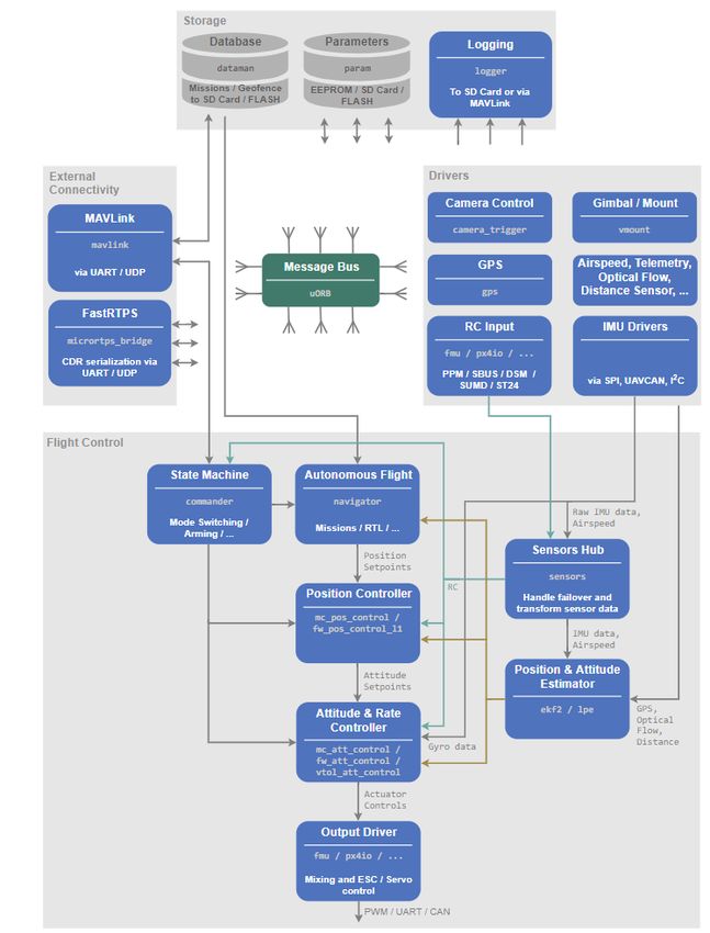
This way flight controller is simply viewed as collection of algorithms packaged in a library.27 Moreover, this code is developed as dependency free header-only pure standard C++11 code requiring no special build to compile simple_flight. To work on any project, the source code is required to be copied to the project that is being worked on. As no additional setup is needed to work with simple_flight, it is advantageous over other flight controllers. Also, simple_flight uses steppable clock which enables the simulation to be paused and still it will not be affected by high variance low precision clock that operating system provides. Further, simple_flight is simple, cross-platform and 100% header-only dependency-free C++ code enabling user to step through from simulator to inside flight controller code within same code base. 6.3.3.1 Control Vehicle control in simple_flight is done by taking in desired input as angle rate, angle level, velocity or position. Each axis of control can be specified with one of these modes. Internally simple_flight uses cascade of PID controllers to finally generate actuator signals. This means position PID drives velocity PID which drives angle level PID which finally drives angle rate PID. 6.3.3.2 State Estimation In current release ground truth from simulator is used for state estimation. Work is in progress to add complimentary filter based state estimation for angular velocity and orientation using 2 sensors (gyroscope, accelerometer) and integrate another library to do velocity and position estimation using 4 sensors (gyroscope, accelerometer, magnetometer and barometer) using EKF. 6.3.4. PX4 PX4 [18] flight code is used by simulator to control a computer modeled vehicle in a virtual world. PX4 can be integrated with different simulators like Gazebo and AirSim to explore flight controller APIs for various UAV functionalities. All PX4 airframes share a single code- base (this includes other robotic systems like boats, rovers, submarines etc.). The complete system design is reactive. Fig. 6.3 shows the block diagram for PX4 1. The functionality is clustered into reusable and exchangeable components. 2. Asynchronous communication is established with message passing. 3. The system is robustly designed to work with varying workload. 6.3.4.1 Flight Stack PX4 flight stack includes guidance, navigation and control algorithms for autonomous drones. It consists of controllers for fixed wing, multirotor and VTOL airframes as well as estimators
28

for attitude and position. As shown in the figure, the building blocks consist of the full pipeline
from sensors, RC input and autonomous flight control (Navigator), down to the motor or servo
control (Actuators).

                      Figure 6.2.: PX4 Flight Stack Block Diagram [18]

    • The estimator takes one or more sensor inputs, combines them, and computes a vehicle
      state (for example the attitude from IMU sensor data).
    • The controller takes a setpoint and a measurement or estimated state (process variable)
      as input. Its goal is to adjust the value of the process variable such that it matches the
      setpoint. The output is a correction to eventually reach that setpoint (for example the
      position controller takes position setpoints as inputs, the currently estimated position
      as the process variable, and attitude and thrust setpoint as output that move the vehicle
      towards the desired position).
    • The mixer takes force commands (e.g. turn right) and translates them into individual
      motor commands. This translation is specific for a vehicle type and depends on various
      factors like motor arrangements with respect to the center of gravity, or the vehicle’s
      rotational inertia.
29 Figure 6.3.: PX4 Block Diagram [18]
30

7. Conclusion
From the discussions in the previous sections, it is clear that technological trends favoring
UAVs have been growing exponentially. Cheaper computation power, improving performance
per dollar and improving performance per watt have been the major contributing factors work-
ing in favour of UAVs. Massive data being generated has a lot of potential to revolutionize
the Robotics and UAV industry in the years to come. From the first phase of this report, it
can be concluded that UAVs find a wide array of application across industry and one of the
major challenges in designing versatile drones is trajectory generation. Some mathematical
functions were discussed weighing their pros and cons and trigonometric sine, cosine were
selected for their smooth trajectory functions.
In the second phase, Simulators have been discussed from a modelling and specifications point
of view, which helps in reducing costs in testing and validation of UAV flight controllers.
An in-depth analysis of multiple simulators is carried out at multiple fronts including but
not limited to long-term support, integrations, effective physical modelling etc. Of these,
AirSim seems to stand out of the rest of them given its highly versatile and powerful APIs,
strong community support and robust system model. The in-depth analysis and documentation
presented in this study shall prove to be useful for future works, which opens the potential of
interfacing Reinforcement Learning with the Simulators to provide a foundation for next level
of Autonomy and Artificial Intelligence.
31

A. (Appendix) AirSim:
   Documentation and Installation
   Instructions
This section and its contents have been quoted from the AirSim official documentation which
is available online at [1]. This documentation has in-depth description of AirSim Code Struc-
ture, System Requirements, APIs, Vehicle and Environment Models, Setup Installation in-
structions and Guide to use the simulator.

A.1. Code Structure

A.1.1. AirLib
Majority of the code is located in AirLib. This is a self-contained library that can be compiled
with any C++11 compiler. AirLib consists of the following components:
   1. Physics engine: This is header-only physics engine. It is designed to be fast and exten-
      sible to implement different vehicles.
   2. Sensor models: This is header-only models for Barometer, IMU, GPS and Magnetome-
      ter
   3. Vehicle models: This is header-only models for vehicle configurations and models. Cur-
      rently it has model for a MultiRotor and a configuration for PX4 QuadRotor in the X
      configuration
   4. Control library: This part of AirLib provides abstract base class for our APIs and con-
      crete implementation for specific vehicle platforms such as MavLink. It also has classes
      for the RPC client and server.

A.1.2. Unreal/Plugins/AirSim
The only portion of AirSim dependent on Unreal engine is the plugin. It is kept isolated
to enable implementation of simulator for other platforms as well. The Unreal code takes
advantage of its UObject based classes including Blueprints.
32
1. SimMode_ classes: To support various simulator modes such as pure Computer Vision
mode where there is no drone. The SimMode classes help implement many different
modes.
2. VehiclePawnBase: This is the base class for all vehicle pawn visualizations.
3. VehicleBase: This class provides abstract interface to implement a combination of ren-
dering component (i.e. Unreal pawn), physics component (i.e. MultiRotor) and con-
troller (i.e. MavLinkHelper).
A.1.3. MavLinkCom
This library is developed by Chris Lovett at Microsoft that provides C++ classes to talk to the
MavLink devices. This library is stand alone and can be used in any project.
A.1.4. Unreal Framework
The following picture illustrates how AirSim is loaded and invoked by the Unreal Game En-
gine:
A.2. System Requirements
System Requirements as per [20]
A.2.1. Hardware Requirements
GPUs such as NVidia 1080 or NVidia Titan series with powerful desktop such as one with
64GB RAM, 6+ cores, SSDs and 2-3 displays (ideally 4K) is recommended. The development
experience on high-end laptops is generally sub-par compared to powerful desktops however
they might be useful in a pinch. Generally laptops with discrete NVidia GPU (at least M2000
or better) with 64GB RAM, SSDs and hopefully 4K display work well. Laptops with only
integrated graphics might not work well.
A.2.2. Software Requirements
• • Unreal Engine
• Windows (Preferable)/ Linux OS
• Anaconda (preferable Python 3.5 or above for APIs)
• ROS
Windows 10 and Visual Studio 2017 are recommended as development environment. This is
because the support for other OSes and IDE is not as mature on the Unreal Engine side.33
A.3. Installation Instructions
1. Download the Epic Games Launcher. While the Unreal Engine is open source and free
to download, registration is still required.
2. Run the Epic Games Launcher, open the Library tab on the left pane. Click on the Add
Versions which should show the option to download Unreal 4.18. If there are multiple
versions of Unreal installed then make sure 4.18 is set to current by clicking down arrow
next to the Launch button for the version.
AirSim binaries can be installed from releases or compile from the source as given below
(Windows, Linux).
A.3.1. Option 1: Download pre-compiled Binaries
Precompiled binaries can be easily downloaded and run to get started immediately. Download
the binaries for the environment of choice from [15]
A.3.2. Option 2: Build AirSim
• Install Visual Studio 2017.
• Make sure to select VC++ and Windows SDK 8.1 while installing VS 2017.
• Start x64 Native Tools Command Prompt for VS 2017.
• Clone the repo: git clone https://github.com/Microsoft/AirSim.git, and go the AirSim
directory by cd AirSim.
• Run build.cmd from the command line. This will create ready to use plugin bits in the
Unreal\Plugins folder that can be dropped into any Unreal project.
A.4. Setup Instructions
A.4.1. Unreal Environment
Setting Up the Unreal Project with Built-in Blocks Environment: To get up and running fast,
the Blocks project that already comes with AirSim can be used. This is not very highly detailed
environment to keep the repo size reasonable but it can be used for various testing and it is the
easiest way to start experimenting with the simulator.34
A.4.2. AirSim Environment: Blocks
Blocks environment is available in repo in folder Unreal/Environments/Blocks and is designed
to be lightweight in size. That means it is very basic but fast.
Here are quick steps to get Blocks environment up and running: (For Windows)
1. Navigate to folder AirSim\Unreal\Environments\Blocks and run update_from_git.bat.
2. Double click on generated .sln file to open in Visual Studio 2017 or newer.
3. Make sure Blocks project is the startup project, build configuration is set to DebugGame_Editor
and Win64. Hit F5 to run.
4. Press the Play button in Unreal Editor.
A.5. Programmatic Control
AirSim exposes APIs so user can interact with the vehicle in the simulation programmatically.
These APIs are used to retrieve images, get state, control the vehicle and so on. The APIs
are exposed through the RPC, and are accessible via a variety of languages, including C++,
Python, C# and Java. These APIs are also available as part of a separate, independent cross-
platform library, so it can be deployed on a companion computer on a UAV. This way the code
can be written and tested in the simulator, and later executed on the real UAV.
To use Python to call AirSim APIs, it is recommended to use Anaconda with Python 3.5 or
later versions and install the following package:
p i p i n s t a l l msgpack−r p c −p y t h o n
A.6. Application Programming Interfaces (APIs)
The following is a list of some of the common APIs
• reset: This resets the vehicle to its original starting state. Note to call enableApiControl
and armDisarm again after the call to reset.
• confirmConnection: Checks state of connection every 1 sec and reports it in Console so
user can see the progress for connection.
• enableApiControl: For safety reasons, by default API control for autonomous vehi-
cle is not enabled and human operator has full control (usually via RC or joystick in
simulator). The client must make this call to request control via API. It is likely that
human operator of vehicle might have disallowed API control which would mean that
enableApiControl has no effect. This can be checked by isApiControlEnabled.35
• isApiControlEnabled: Returns true if API control is established. If false (which is de-
fault) then API calls would be ignored. After a successful call to enableApiControl, the
isApiControlEnabled should return true.
• ping: If connection is established then this call will return true otherwise it will be
blocked until timeout.
• simPrintLogMessage: Prints the specified message in the simulator’s window. If mes-
sage_param is also supplied then it’s printed next to the message and in that case if this
API is called with same message value but different message_param again then pre-
vious line is overwritten with new line (instead of API creating new line on display).
For example, simPrintLogMessage("Iteration: ", to_string(i)) keeps updating same line
on display when API is called with different values of i. The valid values of severity
parameter is 0 to 3 inclusive that corresponds to different colors.
• simGetObjectPose, simSetObjectPose: Gets and sets the pose of specified object in
Unreal environment. Here the object means "actor" in Unreal terminology. They are
searched by tag as well as name. Please note that the names shown in UE Editor are
auto-generated in each run and are not permanent. So if the actor needs to be referred
by name, then its auto-generated name needs to be changed in UE Editor. Alternatively,
add a tag to actor which can be done by clicking on that actor in Unreal Editor and then
going to Tags property, click "+" sign and add some string value. If multiple actors have
same tag then the first match is returned. If no matches are found then NaN pose is
returned. The returned pose is in NED coordinates in SI units with its origin at Player
Start. For simSetObjectPose, the specified actor must have Mobility set to Movable or
otherwise you will get undefined behavior. The simSetObjectPose has parameter tele-
port which means object is moved through other objects in its way and it returns true if
move was successful
A.7. APIs for Multimotor
Multirotor can be controlled by specifying angles, velocity vector, destination position or
some combination of these. There are corresponding move* APIs for this purpose. When
doing position control, we need to use some path following algorithm. By default AirSim
uses carrot following algorithm. This is often referred to as "high level control" because it
specifies high level goal and the firmware takes care of the rest. Currently lowest level control
available in AirSim is moveByAngleThrottleAsync API.
Python Scripts needs to be generated with the AirSim Simulator to perform different maneu-
vers, whereupon specifying parameters such as velocity, angle, position etc, API calls to sim-
ulator can be made. Regarding control of these parameters, these APIs make it easy, as such
parameters can be passed as arguments to function calls in these libraries. (For eg. Velocities
in the X,Y,Z directions can be specified as:
Client.moveByVelocity(vx=x_velocity, vy=y_velocity, vz=z_velocity, duration=duration_of_movement)You can also read