Unemployment Effects of Stay-at-Home Orders: Evidence from High Frequency Claims Data
←
→
Page content transcription
If your browser does not render page correctly, please read the page content below

IRLE WORKING PAPER
                                                                               #101-20
                                                                              April 2020

Unemployment Effects of Stay-at-Home Orders:
Evidence from High Frequency Claims Data

ChaeWon Baek, Peter B. McCrory, Todd Messer, and Preston Mui

Cite as: ChaeWon Baek, Peter B. McCrory, Todd Messer, and Preston Mui. (2020). “Unemployment Effects of
Stay-at-Home Orders: Evidence from High Frequency Claims Data”. IRLE Working Paper No. 101-20.
http://irle.berkeley.edu/files/2020/04/Unemployment-Effects-of-Stay-at-Home-Orders.pdf

http://irle.berkeley.edu/working-papers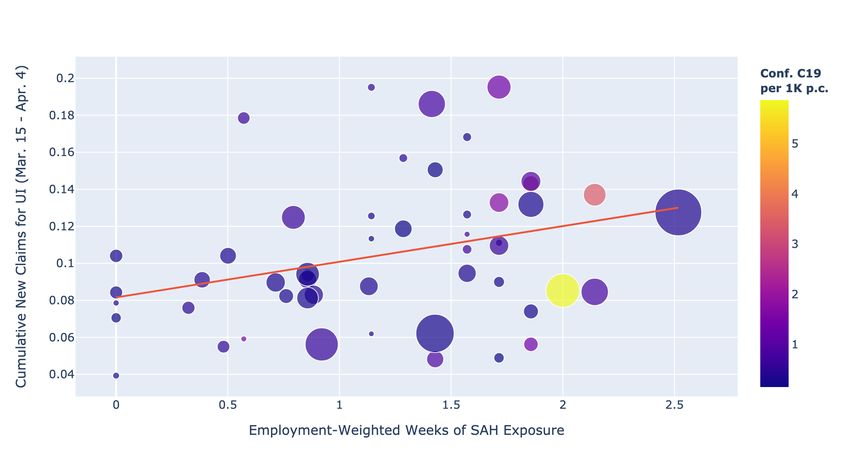
Unemployment Effects of Stay-at-Home Orders:
                Evidence from High Frequency Claims Data

         ChaeWon Baek∗ , Peter B. McCrory∗ , Todd Messer∗ , and Preston Mui∗

                                              April 23, 2020

                                                  Abstract

          Without effective mitigation strategies, epidemiological models project that upwards of 2
      million Americans are at risk of death from the coronavirus pandemic, with many more subject
      to uncertain health complications. Heeding the warning, in mid-March 2020, state and local
      officials in the United States began issuing Stay-at-Home (SAH) orders, instructing people to
      remain at home except to do essential tasks or to do work deemed essential. By April 4th,
      2020, nearly 95% of the U.S. population was under such directives. Over the same three week
      period, initial claims for unemployment spiked to unprecedented levels. In this paper, we use
      the high-frequency, decentralized implementation of SAH policies, along with high-frequency
      unemployment insurance (UI) claims, to disentangle the local effect of SAH policies from the
      general economic disruption wrought by the pandemic that affected all regions similarly. We
      find that, all else equal, each employment-weighted week of Stay-at-Home exposure increased
      a state’s weekly initial UI claims by 1.9% of its employment level. Ignoring cross-regional
      spillovers, this finding implies that, of the 16 million UI claims made between March 14, 2020
      and April 4, 2020, only 4 million are attributable to the Stay-at-Home directives. This evidence
      suggests that the direct effect of SAH orders accounted for a significant, but minority share of
      the overall rise in unemployment claims, and that the majority of the rise in unemployment
      during this period would have occurred in the absence of these orders. This suggests that
      any economic recovery that arises from undoing SAH orders will be limited if the underlying
      pandemic is not resolved.

Keywords: COVID-19, Non-pharmaceutical Interventions, NPIs, Stay-at-Home orders, Unemploy-
ment Effect, UI Claims, Pandemic Curve, Recession Curve.
JEL Codes: C21, C23, E24, E65, H75, I18, J21

   ∗ UC-Berkeley, Department of Economics, Evans Hall, Office 642 (all). Corresponding Author: Peter B. McCrory

(pbmccrory@berkeley.edu). We thank Christina Brown, Yuriy Gorodnichenko, Christina Romer, Maxim Massenkoff,
and Benjamin Schoefer for helpful comments and suggestions.

                                                      1
1 Introduction
To limit the spread and severity of the coronavirus pandemic, officials around the globe have turned
to non-pharmaceutical interventions (NPIs): shutting down schools, restricting economic activities
to those deemed essential, and requiring people to remain at home whenever possible. In mid-
March 2020, Ferguson et al. (2020) issued a report projecting that, in the absence of the effective
implementation of NPI mitigation strategies, more than 2 million Americans were potentially at
risk of death from the COVID-19 respiratory disease, with many more facing uncertain medical
complications in the near- and long-run.
Soon after, state and local officials in the United States began announcing Stay-at-Home (SAH)
Orders, with the earliest announced in the Bay Area, California on March 16th, 2020. Three days
later, the governor of California issued a state-wide order that residents remain in their homes
except to do tasks deemed essential. By March 24th, 2020, more than 50% of the U.S. population
was under such a Stay-at-Home directive (see Figure 1). By April 4th, 2020, 95% of the U.S.
population was under a state or local directive to stay at home, substantially reducing supply of
and demand for locally produced goods and services viewed as nonessential.
At the same time, there was mounting evidence of substantial disruption to labor markets in the
United States. On March 26th, 2020, the preliminary report of initial claims for unemployment for
the week ending March 21st, 2020 was released. In that week, the Department of Labor (DOL)
reported that more than 3.3 million individuals filed for unemployment benefits. For comparison, in
this week, one year prior, there were little more than 200 thousand initial claims for unemployment
insurance.1
The subsequent week (ending March 28th, 2020), initial claims for unemployment once again hit a
new all-time high of approximately 6 million claims. This dramatic increase in claim filings coincided
with a sharp increase in the share of the population under SAH orders, as made clear in Figure 1.
At the same time, the share of the population under a SAH directive increased from 20% to nearly
70%, which begs the question: how much of the increase in UI claims is attributable to the newly
implemented SAH policies?
Unfortunately, looking at these aggregate statistics alone, it is not possible to discern whether and
to what extent the implementation of SAH policies caused the dramatic rise in UI claims. This
is because the increase in unemployment claims can be attributed to a multitude of factors, not
just SAH policies, occurring at the same time. For example, consumer and business sentiment both
declined as the pandemic worsened, with economic uncertainty rising sharply as well. One stark
example of this economic uncertainty was the swift drop in the value of the S&P 500 stock market
1 This was also the first time since the DOL began issuing these reports that the flow into unemployment insurance
exceeded the number of individuals with continuing claims.
2Figure 1: Cumulative Share of Population under Stay-at-Home Order in the U.S.
Sources: Census Bureau, The New York Times; Authors’ Calculations
index, which lost roughly 30% of its value between February 20 and March 16, the first day a SAH
policy was announced in the United States.
This note disentangles the effects of SAH policies from the broader economic disruption brought
on by the coronavirus pandemic. We do so by providing evidence of a direct causal link between
the implementation of SAH policies and the observed increase in UI claims. To the best of our
knowledge, this note is the first systematic study of the causal link between SAH policies and UI
claims in the United States. This is our main contribution.2
The second contribution of this study is illustrative. In what follows, we show that the decentralized
implementation of SAH policies across the U.S. induced high-frequency regional variation as to when
and to what degree local economies were subject to such policies. Our estimates of the effect of such
policies on UI claims provides evidence that this regional variation is useful for understanding the
economic effects of SAH policies. Our empirical design could be useful for studying the effects of SAH
policies on other high-frequency, regionally disaggregated indicators of economic activity.
In this note, we focus on UI claims for three reasons: (1) UI claims are among the highest frequency
indicators of real economic activity—especially as it relates to the labor market; (2) These data are
consistently reported at a subnational level; (3) The data are publicly available.
2 Note that since our variable of interest pertains to the governmental implementation of a stay-at-home policy,
our design does not capture the effects of, for example, social distancing behaviors that may have taken place in the
absence of a government order.
3In our benchmark specification, our outcome variable is cumulative weekly UI claims between March
14 and April 4, divided by state employment. Our measure of SAH exposure is a weighted average
of the number of weeks that each state’s counties were subject to a SAH policy, where the weights
are determined by county employment. In our preferred specification, we find that an additional
week of exposure to SAH policy increases UI claims by approximately 1.9% of a state’s employment
level.
As mentioned, the timing of SAH orders may have occurred concurrently, or been caused by, al-
ternative factors. We therefore consider various control variables and alternative specifications to
show the robustness of this positive relationship. These alternative specifications include: weighting
by state employment; controlling for COVID-19 cases; predicted UI claims based on sectoral com-
position and/or the share of jobs that can be done at home in each state; dropping each state at a
time from the estimation; and changing the horizon over which the treatment and outcome variable
are constructed. We also consider a panel design that allows us to control separately for week fixed
effects between March 14 and April 11.
It is worth pointing out that in our analysis we are unable to distinguish between competing mech-
anisms by which SAH policies might ultimately increase UI claims—for example, either through
the collapse in the supply of goods that require on-site labor and/or through the drop in demand
for high-contact, nonessential goods and services (e.g. live concert musical performances). We leave
this for future research.
Nevertheless, we do provide compelling evidence of one underlying mechanism as it relates to the
demand channel. Estimating event-study regressions using a daily, county-level retail mobility index
(measuring trips to places like restaurants or shopping centers) constructed by Google, we show that
retail mobility fell sharply on the day that SAH policies became effective and remained persistently
low thereafter.3
Across all specifications, we find a consistently positive and statistically significant (oftentimes at
the 1% level) relationship. The range of estimates in the cross-sectional specifications is an increase
in UI claims of 1.9% to 2.2% of state employment for each week a state is subject to a SAH policy;
in our preferred panel specification, the coefficient falls to 1.1%. Our baseline specification yields a
point estimate of 1.9%. This coefficient corresponds to an estimated rise of 4 million claims between
March 14th, 2020 and April 4th, 2020, which accounts for approximately 1/4th of the overall rise
in unemployment claims between March 14th, 2020 and April 4th, 2020. The direct effect of SAH
orders on unemployment is therefore small relative to the aggregate increase in UI claims, suggesting
that a large majority of the increase in unemployment may have occurred in the absence of SAH
orders.
3 The community mobility reports are available at https://www.google.com/covid19/mobility/data_documentation.html
4Related Literature
Our note relates most obviously to the rapidly growing economic literature studying the coronavirus
pandemic, its economic implications, and the policies used to address the simultaneous public health
and economic crises. Broadly speaking, the macroeconomic literature on COVID-19 has split into
two distinct yet highly related strands. Here we provide a representative, albeit not exhaustive,
review.
The first strand of research focuses on the relationship between macroeconomic activity, policy, and
the unfolding pandemic. Gourinchas (2020) and Atkeson (2020) are early summaries of how the
public health crisis and associated policy interventions interact with the economy. Both emphasize
the trade-off between flattening the pandemic curve while steepening the recession curve. Similarly,
Faria–e–Castro (2020) studies the effect of a pandemic-like event in a quantitative DSGE model in
order to assess the economic damage associated with the pandemic as well as the fiscal interventions
employed in the U.S. to attempt to flatten the recession curve. Eichenbaum, Rebelo, and Trabandt
(2020) derive an extension of the standard Susceptible-Infected-Recovered (SIR) epidemiological
model to incorporate macroeconomic effects, formalizing the relationship between the flattening
the pandemic curve and amplifying the recession curve. We view our note as providing causally
identified, empirical support for this theorized relationship between the two curves.
The second strand of research uses high-frequency data to understand the economic fallout wrought
by the coronavirus pandemic. Our note aligns more closely with this strand of the literature. Baker
et al. (2020) show that economic uncertainty measured by stock market volatility, newspaper-based
economic uncertainty, and subjective uncertainty in business expectation surveys rose sharply as the
pandemic worsened. Lewis, Mertens, and Stock (2020) derive a weekly national economic activity
index and show that the coronavirus outbreak has already had a substantial negative effect on the
United States economy. Hassan et al. (2020) use firm earnings calls to quantify the risks to firms
as a result of the coronavirus crisis. Coibion, Gorodnichenko, and Weber (2020) examine how the
pandemic has affected the labor market in general. Using a repeated large-scale household survey,
they show that by April 6th, 2020, 20 millions jobs were lost and the labor market participation
rate had fallen sharply.
Our note also relates to empirical work studying the effect of lockdown policies more specifically. For
example, Hartl, Wälde, and Weber (2020) study the effect of the lockdown in Germany on the spread
of the COVID-19. In contrast to these papers, we use geographic variation to understand the effect
of coronavirus on economic activity. In that respect, our note can be thought of a high frequency
version of Correia et al. (2020), who find that over the long term, NPI policies implemented in
response to the 1918 Influenza Pandemic ultimately resulted in faster growth during the recovery
following the pandemic.
5A closely related paper is Friedson et al. (2020), which uses the state-wide SAH policy implemen-
tation in California along with high frequency data on confirmed COVID-19 cases and deaths to
estimate the effect of this policy on flattening the pandemic curve. Unlike our approach, however,
the authors in this paper use a synthetic control research design to identify the causal effects on this
policy. The authors argue that the SAH policy in California reduced the number of cases by 150K
over three weeks; with their synthetic control, with weights determined by confirmed COVID-19
cases, the authors also perform a back of the envelope calculation to calculate roughly 2-4 jobs lost
over a three week period in California per case saved. In contrast to Friedson et al. (2020), we are
able to directly estimate the causal effect of SAH policies on UI claims. Taking their benchmark
number of cases saved over three weeks, we find that a SAH policy implemented over three weeks
in California would increase UI claims by 6.4 per case saved.4
Another closely related paper is Kong and Prinz (2020), who use high-frequency Google search data
as a proxy for UI claim activity to study the effect of policies closing or limiting restaurants on
unemployment. They find that 29% of the UI claims in the food service industry between March
14th and March 28th were caused by states’ policies closing or limiting bars and restaurants. Their
work differs from ours by focusing on a NPI targeted at a specific sector, and relies on an extremely
high-frequency proxy for UI claims, while the policies we consider are broader and we use actual UI
claims. Nonetheless, both of our results are consistent in finding that NPIs had significant effects on
unemployment, but only account for a small portion of the overall increase in unemployment.
2 Data
2.1 State-Level Stay-at-Home Exposure
We construct a county-level dataset of Stay-at-Home policy implementation based on reporting by
the New York Times. On March 24th, 2020, the New York Times began tracking all cities, counties,
and states in the United States that had issued SAH policies for their residents and the dates that
those orders became effective.5
With this information, we calculate the number of weeks that each county c in the U.S. had been
under a SAH order between day t − k and day t (and counting the day that the policy became
effective).6 We denote this variable with SAHc,s,t,t−k , where s indicates the state in which the
4 UI claims likely understate job losses, since not all workers are eligible for claiming UI. Our baseline estimates
are mostly identified off of variation prior to the passage and implementation of the CARES Act, which expanded
UI coverage.
5 The most recent version of this page is available at https://www.nytimes.com/interactive/2020/us/coronavirus-
stay-at-home-order.html. Over time, the reported information on this site became less granular. Specifically, when a
state issued its own SAH order, the New York Times stopped separately reporting sub-regional orders. We therefore
used The Internet Archive to verify the timing and location of SAH orders as reported in the New York Times.
6 When a city implements a SAH policy, we assign that date to all counties in which that city is located—unless
6county is located. Except when explicitly stated, we drop the t − k subscript and set k to be large
enough so that this variable records the total number of weeks of SAH implementation in county c
through time t.
As an example, consider Alameda County, California. Alameda County was among the first coun-
ties to be under a Stay-at-Home order when one was issued on March 16th, 2020. In this case,
SAHAlameda,CA,M ar.28 = 13/7, as Alameda County had been under Stay-at-Home policies for thir-
teen days. Los Angeles County, California, on the other hand, did not issue a Stay-at-Home policy
before the state of California did so. We therefore set SAHLosAngeles,CA,M ar.28 = 10/7 because a
state-wide order was issued in California on March 19th, 2020.
The previous two examples illustrate how, in some instances, county officials took action before the
state in which they were located did. While we are able to use this county-level variation to study
the impact of SAH policies on retail activity as measured by the Google mobility index, our main
outcome of interest, new unemployment claims, is available to us only at the state level.7
To aggregate county-level SAH policies, we construct a state-level measure of the duration of ex-
posure to SAH orders by taking an employment-weighted average across counties in a given state.
Formally, we calculate:
X Empc,s
SAHs,t ≡ × SAHc,s,t (1)
c∈s
Emps
Employment for each county is the average level of employment in 2018 as reported by the BLS
in the Quarterly Census of Employment and Wages (QCEW).8 One can think of SAHs,t as the
average number of weeks a worker in state s was subject to SAH orders by time t.
Figure 2 reports SAHs,Apr.4 for each state in the U.S. and the District of Columbia. California
had the highest exposure to Stay-at-Home orders, with a value of 2.5, indicating that worker-weeks
of exposure was about two and a half weeks. Conversely, five states (Arkansas, Iowa, Nebraska,
Northa Dakota, and South Dakota) had none of its counties under Stay-at-Home policies by April
4. The average value of SAHs,Apr.4 is 0.4.
of course the county had already issued a SAH order.
7 Some states report sub-state data, but these are not available systematically for the entire country.
8 The annual averages by county in 2019 were, at the time of writing, not yet publicly available.
7Figure 2: Employment-Weighted State Exposure to Stay-at-Home Policies Through Week Ending
April 4
The Employment-Weighted exposure to SAH for a particular state is calculated by multiplying the number of
weeks each county in the state is subject to SAH by the 2018 QCEW average employment share of that county in the
state, and summing over each states’ counties. Sources: Bureau of Labor Statistics, The New York Times; Authors’
Calculations
2.2 Main Outcome Variable: State Initial Claims for Unemployment In-
surance
Our main outcome of interest is initial unemployment claims. Initial unemployment claims are
among the highest-frequency real economic activity indicators available. As discussed in the intro-
duction, initial claims for unemployment for the week ending March 21st, 2020 were unprecedented,
with more than 3 million workers claiming benefits. By the end of that week, very few states or
counties had issued Stay-at-Home orders. Figure 1 shows that by March 21st, 2020, only around
20% of the state had issued such orders. This again illustrates the point that a substantial part of the
economic disruption associated with the coronavirus crisis is likely unrelated to the implementation
of SAH policies.
8Let U Is,t indicate new unemployment claims for state s at time t. In our baseline specification, we
consider the effect of SAH policies on cumulative weekly unemployment claims by state from March
14 to April 4:
U I s,Apr.4 = U Is,M ar.21 + U Is,M ar.28 + U Is,Apr.4 (2)
We then normalize this variable by employment for each state, as reported in the 2018 QCEW, to
arrive out our outcome variable of interest:
U I s,Apr.4
(3)
Emps
3 Empirical Specification
Our baseline specification is a state-level, cross-sectional regression:
U I s,Apr.4
= α + βC × SAHs,Apr.4 + Xs Γ + s (4)
Emps
where Xs is a vector of controls. Our choice of April 4th as the end date for this regressions is
driven by the observation that, by April 4th, approximately 95% of the U.S. population was under
a SAH directive.
An additional reason for preferring April 4th is that over longer horizons, there is greater risk of
omitted variable bias (i.e. Cov[s SAHs,Apr.4 ] 6= 0). A salient example is the rollout of the Paycheck
Protection Program (PPP) on April 3rd.9 This program provided forgivable loans to small businesses
affected by the economic fallout of the pandemic, so long as those loans were used to retain workers.
On the margin, PPP incentivizes firms to not lay off their workers, which would tend to lower UI
claims for the week after April 4th. Depending upon how this interacts with the timing of SAH
implementation, the bias could go in either direction.
In order for β̂C to have a causal interpretation it must be the case that the timing of SAH policies im-
plemented at the state and sub-state level be orthogonal with unobserved factors affecting reported
state-level UI claims. In the baseline specification we consider three important controls.
First, an immediate concern is that the timing of SAH orders is directly related to the severity of
the coronavirus outbreak. These new cases, in turn, affect business directly via lower demand (due
to a sicker population and because people may themselves implement social distancing), depressed
9 The PPP was a central component of the CARES Act, a two trillion fiscal relief package signed into law on
March 27, 2020. The PPP authorized $350 billion dollars in potentially forgivable SBA guaranteed loans.
9household expectations of regional economic growth, and/or store closings. We control for this source
of bias by including the number of coronavirus cases per 1000 people through April 4th.10
Our second control is intended to address the concern that the timing of SAH implementation may
be related to the sectoral composition within each state, and therefore the magnitude of job losses
experienced by that state irrespective of SAH policies. To address this concern, we use a measure
of predicted state-level UI claims as determined by industry composition within each state and the
monthly change in jobs as reported in the national jobs report in March by the BLS. These numbers
are based on a survey reference period that concluded on March 14th, 2020—fortuitously for us,
two days before any SAH policy was announced. Specifically, the measure that we construct is a
Bartik-style control:
X
Bs = ∆ ln Empi,M arch × ωi,s (5)
i
where Empi,M arch is the monthly percentage change in employment in industry i (3-digit NAICs)
for the month of March. ωi,s is the share of employment in industry i in the state, as reported in
the QCEW for 2018.
Third, we control for a state-level work-at-home index. Dingel and Neiman (2020) construct an
index denoting the share of jobs that can be done at home by cities, industries, and countries. We
aggregate their industry-level (2-digit NAICs) index to the state-level, by taking an employment-
weighted average. Precisely, we calculate the state-level work-at-home index as follows:
X Empi,s
W AHs = W AHi , (6)
i
Emps
where i denotes industry, and s denotes state.
States with fewer jobs that can be done at home may be more affected by SAH policies. Addition-
ally, it may be the case that states with a higher work-at-home index may have been willing to
implement SAH policies earlier for political economy reasons. If this index is correlated with the
number of initial UI claims issued by the state, then failing to include this control would introduce
bias.11
10 We rely upon confirmed COVID-19 cases as compiled at the county-by-day frequency by USAFacts. USAFacts is a
non-profit organization that compiles these data from publicly available sources, typically from daily reports issued by
state and local officials. See https://usafacts.org/visualizations/coronavirus-covid-19-spread-map/ for more details.
11 As for the first point, in unreported regressions, we study whether the effect of SAH policies depends upon the
value of the work-at-home index; we find no evidence that this is the case.
10β̂C , our coefficient of interest, has the natural interpretation of the number of individuals that
claimed unemployment insurance as a percent of a state’s employment level for each week that that
state remained under a Stay-at-Home order through April 4th, 2020.12
Given the unprecedented increase in UI claims during our sample, another concern is that institu-
tional capacity to process new UI claims may vary by state systematically with the implementation
of SAH policies. More specifically, if greater exposure to SAH policies tends to make it more difficult
for states to process UI claims, then state reported claims in any given week may understate the
number of people seeking UI after job loss. While we are unable to control for this concern explicitly,
we do note that this source of omitted variable bias would tend to bias our estimates downward,
making our estimate of the effect of SAH policies on UI claims a lower bound.
Figure 3: Box Plots by Week of Initial UI Claims Relative to Employment for Early and Late
Adopters of SAH Policies
For each state we calculate SAH exposure through April 4th by multiplying the number of weeks each county
was subject to SAH through April 4 by the 2018 QCEW average employment share of that county in the state, and
summing over each state’s counties. Early adopters are those states in the top quantile of SAH exposure and late
adopters are those states in the bottom quartile. Sources: Bureau of Labor Statistics, Department of Labor, and The
New York Times; Authors’ Calculations.
To illustrate our empirical design, in Figure 3 we compare the evolution of UI claims to state
employment of "early adopters," defined as those states being in the top quartile of SAH exposure
through April 4, 2020, to those of "late adopters," defined as those states being in the bottom
13
quartile. This figure provides graphical evidence of the main result of our paper: in the first few
weeks, early adopters initially had a higher rise in unemployment claims relative to late adopters. By
12 It is possible for workers to be double-counted in the QCEW if they hold multiple-jobs. This would make our
estimate a lower bound on the effect of SAH policies.
13 The upper and lower edges of the boxes denote the interquartile range of each group, with the horizontal line
denoting the median. As is standard, the "whiskers" denote the value representing 1.5 times the interquartile range
boundaries.
11the week ending April 4th, 2020, the relative effect of adopting SAH orders early largely disappears,
reflecting the fact that by this point approximately 95% of the U.S. population was under a SAH
order.
This figure also illustrates a broader point of our paper: that there may be limited economic relief
from removing SAH policies so long as the public health crisis persists. In early weeks, late adopters
experienced historically unprecedented levels of UI claims even though early adopters had higher
claims on average. For example, consider the week ending March 28. Here the difference between
the median value of the two groups was approximately 1% of state employment; in that week, the
median value of initial claims to employment for late adopters was roughly 3%, despite close to
zero SAH exposure by this point. By April 4th, this difference almost completely disappears. Late
adopters, who were under SAH orders for a much shorter period of time (or not at all, in some
cases), converged to similar levels of unemployment claims relative to employment.
4 Results
We present results for our benchmark specification in Table 1. Column (1) shows the univariate
specification, with no controls. The point estimate of approximately 1.9% (SE: 0.67%) implies that
a one-week increase in SAH orders raises the number of claims as a share of state employment by
1.9%. Figure 4 displays this result graphically, with shading denoting the intensity of the coronavirus
pandemic and the size of the bubbles representing population.
Column (2) controls for the number of confirmed COVID-19 cases per one thousand people. To the
extent that COVID-19 infections increased the probability of implementing SAH orders and had
negative effects on employment, then we should expect to see the coefficient fall. We find that there
is almost no effect of COVID-19 cases after controlling for our measure of SAH exposure.
Columns (3) and (4) include two additional controls. Only the WAH index is marginally significant,
but our point estimate is largely unchanged. This is largely due to the lack of correlation between
the WAH index and the timing of implementing SAH policies. In column (5), we control for only
the WAH variable (the only significant one), and find that our SAH exposure variable retains its
significance and magnitude.
Our results support the idea that flattening the pandemic curve implies a steepening of the re-
cession curve in the absence of any government support (Gourinchas, 2020). However, the relative
contribution of SAH policies to the steepening of the recession curve steepens is small, according
to our estimates.14
14 In unreported calculations, we find that the implied the cost in lost labor income is far outweighed by the benefits
as calculated by Greenstone and Nigam (2020).
12Figure 4: Scatterplot of SAH Exposure to Cumulative Initial Weekly Claims for Weeks Ending
March 21 thru April 4
The Employment-Weighted exposure to SAH for a particular state is calculated by multiplying the number of
weeks each county in the state is subject to SAH, and multiplying by the 2018 QCEW average employment share
of that county in the state, and summing over the states’ counties. UI claims are cumulative new claims during the
period, divided by average 2018 QCEW average employment in the state.
Size of bubbles proportional to state population; Color gradient of each observation determined by the number
of confirmed COVID-19 cases per thousand people.
Sources: Bureau of Labor Statistics, Census Bureau, The New York Times, USAFacts.org, Department of Labor;
Authors’ Calculations
We calculate our estimate of the number of UI claims between March 14 and April 4 attributable
to SAH orders as
X
\
AggClaims = β̂C × SAHs,Apr.4 × Emps (7)
s
where s indexes a particular state. This yields an estimate of 4 million UI claims.15
As mentioned previously, it is not immediately obvious whether the effect we find is a result of the
SAH orders directly. It could be the case that even in the absence of imposing SAH orders, states
15 Alternatively, one could construct an estimate of the implied number of UI claims between March 14 and April
4 by evaluating SAHs,Apr4. at its sample mean. This yields an estimate of 3.25 million UI claims.
13Table 1: Effect of Stay-at-Home Orders on Cumulative Initial Weekly Claims Relative to State
Employment for Weeks Ending March 21 thru April 4, 2020
(1) (2) (3) (4) (5)
SAH Exposure thru Apr. 4 0.0192∗∗∗ 0.0197∗∗ 0.0196∗∗ 0.0192∗∗ 0.0208∗∗∗
(0.00669) (0.00747) (0.00749) (0.00715) (0.00632)
COVID-19 Cases per 1K -0.000816 -0.000796 0.00294
(0.00502) (0.00505) (0.00572)
Bartik-Predicted Job Loss -4.400 -2.229
(9.174) (7.511)
Work at Home Index -0.372+ -0.346
(0.207) (0.210)
Constant 0.0816∗∗∗ 0.0816∗∗∗ 0.0535 0.197∗∗ 0.202∗∗∗
(0.00851) (0.00858) (0.0556) (0.0805) (0.0753)
Adj. R-Square 0.0810 0.0622 0.0501 0.0797 0.112
No. Obs. 51 51 51 51 51
Dependent variable in all cross-sectional regressions is our measure of cumulative new unemployment claims as
a fraction of state employment, as calculated in Equation (3). Interpretation of the SAH Exposure coefficient is the
effect on normalized new UI claims of one additional week of state exposure to SAH.
Robust Standard Errors in Parentheses
+ p < 0.10, ** p < 0.05, *** p < 0.01
would still see a dramatic rise in unemployment claims due to, for example, worsening expectations
of future economic activity. We test whether this is the case by examining the effect of SAH orders
on daily-frequency data from Google’s Community Mobility Report, which measures changes in
visits and duration of visits to grocery stores, retail, work, etc.16,17 We use the mobility index for
retail. If there were no effect of SAH orders on mobility then it is possible the effect on UI claims
would have occurred in the absence of mandated SAH orders.
We estimate event studies of the following form:
K
X
M obilityc,t = αc + φt + βk SAHc,t+k + Dc,t + Dc,t + εc,t (8)
k=K
where M obilityc,t represents the Google retail mobility index in county c on day t, and SAHc,t is a
dummy variable equal to 1 on the day a county imposes SAH orders. We set K = −8 and K = 14.
The sample is unbalanced, as some counties did not impose SAH orders until April. Hence, we
include “long-run” dummy variables, Dc,t and Dc,t .18 The event study is estimated over the period
16 https://www.google.com/covid19/mobility/
17 Note that data is missing for some days in counties. When possible, we linearly interpolate the mobility measure.
Excluding counties with missing values yields the same result; this figure is available from the authors upon request.
18 D
c,t is equal to 1 if a county imposed SAH orders at least K days prior. D c,t is equal to 1 if a county will impose
14February 15th through April 10th, 2020.
Results are presented in Figure 5. We first emphasize, rather surprisingly, the lack of any pretrend
prior to SAH orders. This does not mean that counties did not experience changes in mobility, but
rather it was not systemically related to county-specific SAH orders. The day of the SAH orders,
we see an immediate decline of 5% in retail mobility. This falls further to 10% the day after SAH
orders, and stays persistently low henceforth.19
We take both the lack of pre-trend and the persistent effects of SAH orders via this event study
specification as additional evidence in support of SAH orders have direct, causal effects on unem-
ployment claims, in part through its reduction on retail sales (which is proxied for by the decline
in the retail mobility index).
Figure 5: County Retail Mobility Event Study
The mobility measure is the Google county-level retail community mobility index, which measures visits and
duration of visits to retail establishments. The time unit is days, and the index is normalized to the day before the
SAH order in a county went into effect.
Standard Errors Two-Way Clustered by County and Week
Sources: Google, The New York Times; Authors Calculations
SAH at least K periods in the future.
19 Restricting the sample to exclude never-takers yields the same result. This design identifies the mobility effects off
of counties that ultimately implemented SAH policies but at different times. In an even more restrictive specification,
we estimate the model with time-by-state fixed effects, which yields the same result, albeit with slightly larger
standard errors. The time-by-state fixed effect specification identifies the retail mobility effect off of within-state
differences in the timing of county-level SAH policies. These results are available upon request.
155 Robustness
5.1 Alternative Cross-Sectional Specifications
The first type of robustness check we do is varying the horizon over which the cross-sectional
regression is estimated, considering two natural alternative specifications: a two week horizon and
a four week horizon. For the two week horizon specification, we consider cumulative initial claims
between March 14 and March 28 regressed on SAH exposure over the same window; for the four
week specification, the end date is April 11. Because the work-at-home index was the only significant
control variable in Table 1, we only report results with this control variable.20
Columns (1) and (2) of Table 2 report the results from varying the horizon over which the model
is estimated. Relative to our baseline result of 1.9%, estimating the model over just two weeks
increases the point estimate to 1.85% (SE: 0.78%). Conversely, when the model is estimated over a
four week horizon, the point estimate is 1.9% (SE: 0.55%).
Table 2: Effect of Stay-at-Home Orders on Cumulative Initial Weekly Claims Relative to State
Employment: (i) 2-Week Horizon, (ii) 4-Week Horizon, (iii) Weighted Least Squares
(1) (2) (3)
Mar. 14 - Mar. 28 Mar. 14 - Apr. 11 WLS
SAH Exposure (varied horizons) 0.0185∗∗ 0.0191∗∗∗ 0.0221∗∗∗
(0.00783) (0.00552) (0.00529)
Work at Home Index -0.158 -0.492∗∗ -0.486∗∗
(0.160) (0.244) (0.224)
Constant 0.110+ 0.271∗∗∗ 0.247∗∗∗
(0.0574) (0.0863) (0.0815)
Adj. R-Square 0.0421 0.126 0.124
No. Obs. 51 51 51
The Employment-Weighted exposure to SAH for a particular state is calculated by multiplying the number of
weeks each county in the state is subject to SAH with the 2018 QCEW average employment share of that county in
the state, and summing over each states’ counties. UI claims are cumulative new claims during the period, divided
by average 2018 QCEW average employment in the state.
Robust Standard Errors in Parentheses
+ p < 0.10, ** p < 0.05, *** p < 0.01
In Column (3) of Table 2 we estimate the effect of SAH exposure on UI claims, over the same three
week horizon as in the benchmark case, weighting observations by state-level employment from the
QCEW in 2018 (an approached advocated for by some papers in the local multiplier literature).21
Here, we control only for the work-at-home index. The point estimate from the WLS regression is
20 Asin Table 1, the point estimate on SAH exposure is unaffected by these additional controls.
21 Foropposing views, consider Ramey (2019) and Chodorow-Reich (Forthcoming). See also Solon, Haider, and
Wooldridge (2015).
16elevated slightly relative to the benchmark specification: 2.21% (SE: 0.53%). Regardless, weighting
delivers quantitatively similar estimates.
5.2 Influence of Specific States
One may also be concerned that individual states’ responses, either in terms of rising unemployment
claims or SAH policies, is driving our results. To understand whether this is the case, we replicate
our regressions from above dropping one state at a time. The resulting coefficient estimates for βC
are available in Figure 6.
Figure 6: Benchmark Specification Estimated Dropping One State at a Time
The estimate of βC in (4) when individual states are dropped from the regression.
The key outlier is Nevada. Dropping Nevada raises the point estimate by nearly a third. Nevada
did not have a SAH in place until the week ending April 4th. Specifically, the governor of Nevada
instituted a state-wide SAH order on April 3rd. However, due to the importance of tourism to the
economy of Nevada (in particular, Reno and Las Vegas), initial unemployment claims began to rise
well before the SAH order was implementing. It is therefore unsurprising that dropping this state
raises the estimate of β̂C .
175.3 Panel Specification
One concern with the cross-sectional specifications in the preceding analysis is that there is some
unobserved aggregate factor that is inducing large increases in UI claims at the same time that
states and local municipalities are implementing SAH policies. To address this concern, we employ
a panel specification, which allows us to control for week to week fixed effects.
We modify the specification so that the outcome variable is the flow value of initial claims on
date t and the SAH policy treatment is the share of the current week that a state was subject to
SAH policies, where we take a weighted average of county-level exposure as before. Specifically,
we estimate the following fixed effects panel regression on weekly observations for the week ending
January 4 through the week ending April 11.
U Is,t
= αs + φt + βP × SAHs,t,t−7 + Xs,t Γ + s,t (9)
Emps
We consider a variety of state-time controls. We include two lags of SAHs,t,t−7 to account for
dynamics in the effect of SAH policies on unemployment claims.22 Additionally, we include the share
of the population that works from home, the number of confirmed cases per one thousand people,
and the Bartik-style employment control from before. Each of these three controls is interacted with
a dummy equal to one after March 21st, 2020.23
Table 3 provides our estimate of β̂P , the effect of implementing a SAH policy for one week on
weekly UI claims as a percent of the state’s employment. Given how we structure the cross-sectional
regression, β̂P and β̂C are each estimating the same population moment, so we should expect these
two estimates to be similar. In Column (4), where we include all controls, we find that β̂P is 1.1%
(SE: 0.32%), somewhat lower than our baseline cross-sectional estimates.
6 Conclusion
While non-pharmaceutical interventions (NPIs) are necessary to flatten the spread of viruses such
as COVID-19, they likely steepen the recession curve. But to what extent? We provide estimates
of how much one prominent NPI disrupts the labor markets in the short run.
In this note, we investigated the effect of Stay-at-Home (SAH) orders on new unemployment claims
in order to quantify the causal effect of non-pharmaceutical interventions (i.e., flattening the pan-
22 The coefficient estimates for the lags are small and insignificant, and so we do not report them.
23 Note that because our measures of work-from-home and employment loss are constant across time, we are
controlling for the relative effect of each from before March 21st.
18Table 3: Panel Specification: Effect of Stay-at-Home Orders on Initial Weekly Claims Relative to
State Employment
(1) (2) (3) (4)
SAH Exposure Current Week 0.00885∗∗ 0.0104∗∗∗ 0.0109∗∗∗ 0.0106∗∗∗
(0.00353) (0.00321) (0.00317) (0.00316)
Post-March21 x Work at Home Index -0.110+ -0.125∗∗
(0.0607) (0.0586)
Pre-March21 x COVID-19 Cases per 1K -0.0125
(0.0214)
Post-March21 x COVID-19 Cases per 1K 0.00148∗∗
(0.000719)
Post-March21 x Bartik-Predicted Job Loss -0.457
(2.250)
Constant 0.00909∗∗∗ 0.0102∗∗∗ 0.0221∗∗∗ 0.0227∗∗∗
(0.000487) (0.000594) (0.00647) (0.00762)
Lag SAH N Y Y Y
State FE Y Y Y Y
Week FE Y Y Y Y
Adj. R-Square 0.821 0.818 0.824 0.824
No. Obs. 765 663 663 663
The Employment-Weighted exposure to SAH for a particular state is calculated by multiplying the share of the
current week each county in the state is subject to SAH by the 2018 QCEW average employment share of that county
in the state, and summing over each states’ counties. UI claims are cumulative new claims during the period, divided
by average 2018 QCEW average employment in the state.
Standard Errors Clustered by State in Parentheses
+ p < 0.10, ** p < 0.05, *** p < 0.01
demic curve) on economic activity (i.e., steepening the recession curve). We leverage geographic
and time variation in when regions chose to implement SAH orders.
Between March 14th and April 4th, the share of workers under such orders rose from 0% to almost
95%. This rise was gradual, with new areas implementing such orders on a daily basis. We couple
the induced regional variation in SAH implementation along with high-frequency unemployment
claims data to quantify the resulting economic disruption.
We find that a one-week increase in stay-at-home orders raises unemployment claims by 1.9% of
employment. This accounts for 4 million unemployment insurance claims, about a quarter of the
total unemployment insurance claims during this period. This implies that the bulk of the increase in
unemployment associated with coronavirus crisis was due to other channels, such as, for example,
decreased consumer sentiment, stock market disruptions, and social distancing that would have
occurred in the absence of government orders. We see our paper as providing tentative evidence
that removing government SAH orders may only a fraction of the economic disruption arising from
19the coronavirus pandemic while at the same time exacerbating the public health crisis, and that
the economic disruption will persist until the pandemic itself is resolved.
20References
Atkeson, Andrew. 2020. “What will be the economic impact of COVID-19 in the US? Rough
estimates of disease scenarios.” No. w26867, National Bureau of Economic Research.
Baker, Scott R, Nicholas Bloom, Steven J Davis, and Stephen J Terry. 2020. “COVID-Induced
Economic Uncertainty.” No. w26983, National Bureau of Economic Research.
Chodorow-Reich, Gabriel. Forthcoming. “Regional Data in Macroeconomics: Some Advice for Prac-
titioners.” Journal of Economic Dynamics and Control .
Coibion, Olivier, Yuriy Gorodnichenko, and Michael Weber. 2020. “Labor Markets during the
COVID-19 Crisis: A Preliminary View.” No. w227017, National Bureau of Economic Research.
Correia, Sergio, Stephan Luck, Emil Verner et al. 2020. “Fight the Pandemic, Save the Economy:
Lessons from the 1918 Flu.” No. 20200327, Federal Reserve Bank of New York.
Dingel, Jonathan I and Brent Neiman. 2020. “How many jobs can be done at home?” No. w26948,
National Bureau of Economic Research.
Eichenbaum, Martin S, Sergio Rebelo, and Mathias Trabandt. 2020. “The macroeconomics of
epidemics.” No. w26882, National Bureau of Economic Research.
Faria–e–Castro, Miguel. 2020. “Fiscal Policy during a Pandemic.” No. 2020-006d, Federal Reserve
bank of St. Louis.
Ferguson, Neil M., Daniel Laydon, Gemma Nedjati-Gilani, Natsuko Imai, Kylie Ainslie, Marc
Baguelin, Sangeeta Bhatia, Adhiratha Boonyasiri, Zulma Cucunubá, Gina CuomoDannenburg,
Amy Dighe, Ilaria Dorigatti, Han Fu, Katy Gaythorpe, Will Green, Arran Hamlet, Wes Hins-
ley, Lucy C Okell, Sabine van Elsland, Hayley Thompson, Robert Verity, Erik Volz, Haowei
Wang, Yuanrong Wang, Patrick GT Walker, Caroline Walters, Peter Winskill, Charles Whittaker,
Christl A Donnelly, Steven Riley, and Azra C Ghani. 2020. “Impact of non-pharmaceutical inter-
ventions (NPIs) to reduce COVID19 mortality and healthcare demand.” manuscript, Imperical
College.
Friedson, Andrew I, Drew McNichols, Joseph J Sabia, and Dhaval Dave. 2020. “Did California’s
Shelter-in-Place Order Work? Early Coronavirus-Related Public Health Benefits.” Working Paper
26992, National Bureau of Economic Research.
Gourinchas, Pierre-Olivier. 2020. “Flattening the pandemic and recession curves.” Working paper.
Greenstone, Michael and Vishan Nigam. 2020. “Does Social Distancing Matter?” No. 2020-26,
University of Chicago, Becker Friedman Institute for Economics Working Paper.
21Hartl, Tobias, Klaus Wälde, and Enzo Weber. 2020. “Measuring the impact of the German public
shutdown on the spread of COVID19.” Covid economics, vetted and real-time papers, CEPR
press, 1, 25-32.
Hassan, Tarek Alexander, Stephan Hollander, Laurence van Lent, and Ahmed Tahoun. 2020. “Firm-
level Exposure to Epidemic Diseases: Covid-19, SARS, and H1N1.” No. w26971, National Bureau
of Economic Research.
Kong, Edward and Daniel Prinz. 2020. “The Impact of Non-Pharmaceutical Interventions on
Unemployment During a Pandemic.” No. 3581254, SSRN.
Lewis, Daniel, Karel Mertens, and James H Stock. 2020. “US Economic Activity during the Early
Weeks of the SARS-Cov-2 Outbreak.” No. w26954, National Bureau of Economic Research.
Ramey, Valerie A. 2019. “Ten Years after the Financial Crisis: What Have We Learned from the
Renaissance in Fiscal Research?” Journal of Economic Perspectives 33 (2):89–114.
Solon, Gary, Steven J Haider, and Jeffrey M Wooldridge. 2015. “What are we weighting for?”
Journal of Human resources 50 (2):301–316.
22You can also read