Unsupervised Machine learning methods for city vitality index - arXiv.org
←
→
Page content transcription
If your browser does not render page correctly, please read the page content below
Unsupervised Machine learning methods for city vitality index
                                                       Jean-Sébastien Dessureault, Jonathan Simard, and Daniel Massicotte

                                         Université du Québec à Trois-Rivières, Department of Electrical and Computer Engineering,
                                         3351, Boul. des Forges, Trois-Rivières, Québec, Canada
                                         Laboratoire des Signaux et Systèmes Intégrés
arXiv:2012.12082v2 [cs.LG] 29 Jan 2021

                                         {sebastien.dessureault, jonathan.simard, daniel.massicotte}@uqtr.ca

                                         Keywords: smart city, intelligent urbanism, district vitality index, k-mean algorithm, random forest algo-
                                         rithm, genetic algorithm

                                         ABSTRACT
                                         This paper concerns the challenge to evaluate and predict a district vitality index (VI) over the years. There
                                         is no standard method to do it, and it is even more complicated to do it retroactively in the last decades.
                                         Although, it is essential to evaluate and learn features of the past to predict a VI in the future. This paper
                                         proposes a method to evaluate such a VI, based on a k-mean clustering algorithm. The meta parameters of
                                         this unsupervised machine learning technique are optimized by a genetic algorithm method. Based on the
                                         resulting clusters and VI, a linear regression is applied to predict the VI of each district of a city. The weights
                                         of each feature used in the clustering are calculated using a random forest regressor algorithm. This method
                                         can be a powerful insight for urbanists and inspire the redaction of a city plan in the smart city context.

                                         1    Introduction                                            in [25] made a good review of the literature at this
                                                                                                      time. Since then, the GIS are a very useful tool to
                                         Cities are constantly evaluating. Too often, several         every system that must manage geographical data.
                                         districts in a city has been forgotten for years and
                                         without warning, they are devitalized. It is often too       The concept of smart city came later at the end of
                                         late to act. People and businesses are leaving this          the 90’s [12] [24]. One of the first smart city was
                                         district because of many factors such as the disuse of       Singapore. Many others were following: Suwon,
                                         the houses and the buildings, the bad economic ac-           Seoul (Korea), Taipei (Taiwan), Mikita (Japan),
                                         tivities, the criminality rate, and so on. Even though       Waterloo and Calgary (Canada), Glasgow (Scot-
                                         it is easy to note when a district is already devi-          land), New-York (USA) and Teheran (Iran), to
                                         talized, urbanists do not have some good tools to            name a few [31]. There are mainly three new soft-
                                         predict which district will be devitalized, and when.        ware tools/technologies that allow smart cities to
                                         Historically, the firsts relevant publications were          progress: Big data, Internet of things (IoT) and ar-
                                         made between 1960 and 1980. The works of Donald              tificial intelligence (AI). Talking about Big data and
                                         Appleyard for instance with a study named "Styles            IoT, a study [8] present the case of Santander, Spain.
                                         and methods of structuring a city" [4] was aiming            A platform named "SmartSantander" has made this
                                         to explain different city patterns according to some         city one of the most connected in the world, with
                                         features like the level of education, the age, the sex       its 15,000 sensors (1,200 nodes) over its territory.
                                         and so on. Having back then very few processing ca-          Many sensors are statics and some others are mobile
                                         pacities, those works was preparing a new numeric            (mounted on some bus, taxis, or police cars, for in-
                                         era for urbanism.                                            stance). A big data platform named "CiDAP" was
                                         In the late 70s, a paper [21] introduced some concept        created especially for the city of Santander. Zam-
                                         that will become a Geographical Information System           poglou et al. in [37] present a good review of those
                                         (GIS). There were many publications at the begin-            useful technology for smart cities. Artificial intel-
                                         ning of the 80’s studying those new GIS. Muehrcke            ligence is also a must for intelligent cities. Ma-

                                                                                                  1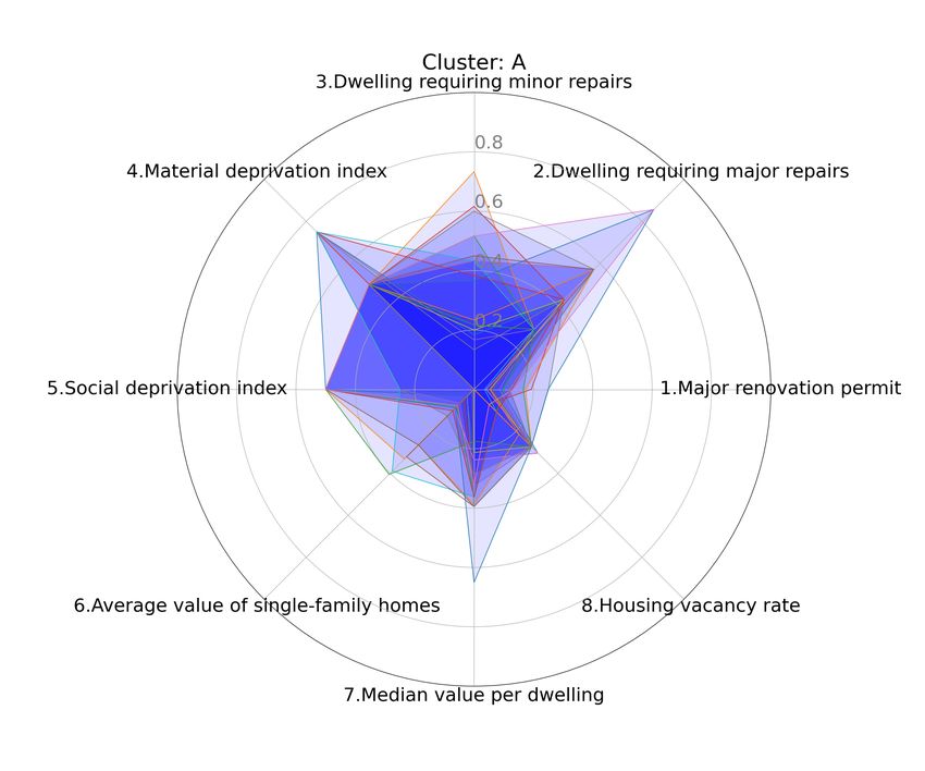
chine learning (ML) techniques like clustering [3]            dimensional grid. From this grid, some simulation
[15] [13] [5], neural networks [27] [36], Bayesian net-       can be run according to some previously defined (or
works [20] [23], cellular automata [9] [28] [36] and          learned) rules. The results of those simulation can
genetic algorithms [14] [33] [18] are very useful in          give some hints of what the territory will look like
this field. Learning from features of the past is the         in the future. Obviously, the cellular automaton is
main strength of ML. Clustering allows to regroup             used combined with some other artificial intelligence
similar features. Neural networks are useful to make          techniques to give some more complete results [22]
some non-linear regressions. Bayesian networks can            [30].
compute probabilities of some future event. Cellular          There is no standard for the evaluation and the pre-
automata allow to simulate a two dimensions geo-              diction of a vitality index (VI). Some papers [2]
graphical map. Finally, genetic algorithms (GA) are           [1] [11] refer to VI, defining their own set of fea-
useful to optimize different types of configuration.          tures (both qualitative and qualitative) and meth-
In the large spectrum of smart cities is the intelli-         ods. Since each city does not archive the same data
gent urbanism [6] [29] [26] [35]. This specific part          over the years, it is difficult to establish a standard
of smart cities aims to help urbanists to read better         set of features for the evaluation of a VI. Each city
their city features and to predict how the urban ter-         must use the consistent data available from the last
ritory will change. There are some paper studying             decades. Being inspired by the previous works, this
different city district indexes. They all study some          paper proposes a method based on ML algorithms to
geographical region and geolocalized features from            define, evaluate, and predict a VI in Trois-Rivières
the past to predict what will happen in the future.           city. It shows the methodology for data preprocess-
The case of Attica (Athens area) in which they pre-           ing such as normalise and represent features, and to
dict urban growth was proposed in [15]. Their work            fill some gap. It defines how both supervised learn-
aims to presents an artificial intelligence approach          ing and unsupervised learning were used to calcu-
integrated with GIS for modeling urban evolution.             late the VI and to make some prediction through
They use a fuzzy logic system using a c-means clus-           years. The usage of a k-means algorithm (unsuper-
tering algorithm to divide the territory using fuzzy          vised learning) that partially defines the index will
frontiers. In this system, each geographical posi-            be proposed. The usage of a feature-weighted in-
tion has a level of membership defined by a mem-              puts with stochastic gradient descent technique, will
bership function [34]. The clusters represent a spe-          also be explained. Finally, we will see how a GA is
cific level of urban growth. This system also uses a          used to optimize the clustering parameters. At the
multilayers neural network (MNN) to learn and pre-            end, this proposed method based on ML algorithms
dict urban growth in the Attica area, by analyzing            provides some good insights for urbanists.
population changes over time and by building pat-             The next sections of this paper are organized with
terns. All the geographical data are managed by a             the following structure: Section 2 describes the pro-
GIS. Amongst many features, 9 has been selected to            posed methodology. Section 3 presents the results.
feed the system: population, population growth in             Section 4 discusses about the results and their mean-
the decade, number of buildings, number of building           ing and Section 5 concludes this research.
growth in the last decade, use of residential sector,
use of commercial sector, use of industrial sector,
use of public sector, other uses. The results shown           2     The proposed method for
a clear profile for each district. For instance, for
group “A”, there is the strongest population growth
                                                                    the vitality index
rate (54.6%). Buildings growth rate is also high at
96.5%. The residential use of the land is high at             2.1    Selected features
91.2%. We can conclude that group “A” represents              According to the Trois-Rivières urbanists, the “vi-
a residential district in full growth. Data from the          tality” of a district can be defined by the strength of
past was learned and used to predict growth rate of           its economy, the health and social status of its cit-
each district in the future. A very strong correlation        izen. Unlike the urban growth index, which tells if
between real and predicted features was shown.                a territory is occupied by urban space, the VI index
Some other papers are doing a similar work, but they          refers to the economic health of an urban territory
model the territory using a cellular automaton [16]           and to the social condition of its citizens. This paper
[32]. This is a good approach when features can               aims to define the VI, to evaluate it according to the
be precisely geolocalized. In this case, it is possi-         Trois-Rivières city features and predict this index
ble to extract information and place it into a two-           for each targeted district in the future. In urbanism

                                                          2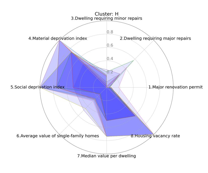
context, we have access to massive data information.         This algorithm’s parameters are optimized with a
The first step was to prioritize and select the right        GA. Afterward, having all the VI for three years
features needed to calculate a VI. This was done             2006, 2011 and 2016 in a 10 years range, the method
in collaboration with urbanism experts. They have            based on this model architecture can predicted the
selected the features they thought could have a sig-         district evolution in the future. This prediction is
nificant influence on a VI. Table 1 presents the eight       made using a linear regression.
selected features and the pre-processing applied on          Fig. 1 shows the block diagram of the dataflow and
them.                                                        the ML used represented in 3 steps: (1) GA and
  As shown in Table 1, pre-processing as been ap-            clustering, (2) for neural network, and (3) linear
plied to each feature. First, every feature has been         regression.
normalized using a MinMax function based on the
assumption that each feature has same importance
in the VI. Eq. 1 shows the MinMax normalization
formula. It simply normalizes a number to get a 0
to 1 range, associating the smallest value to 0 and
the highest to 1.

Table 1: Vitality index features and their pre-
processing

                                                             Figure 1: Proposed framework design in three steps
                                                             (1) genetic algorithm and clustering, (2) for neural
                                                             network, and (3) linear regression.

                                                             To have a whole system to evaluate and predict a
                                                             VI, several types of ML algorithms must be used.
This is easier way to calculate the index and to
present features on the same scale using different           2.3    Unsupervised learning                  —      k-
graphics. The presentation of the features is es-                   means clustering
pecially important since it must be interpreted by
urbanists. To have a better feature distribution, a          To determine the VI, it is necessary to use an unsu-
logarithmic function is used to scale the feature in         pervised learning technique since there is no tagged
logarithmic scale. Some features have been inverted          label for each input data. This algorithm will assign
to keep the consistency: 0 is always the worst fea-          to each district a cluster reference letter, according
ture value and 1 is always the better feature value.         to a similarity level of their features. A k-means
Finally, some average values were used when no data          algorithm has been used to determine the clusters.
were available.                                              Eq. 2 defined the k-means clustering equation where
                                                             J is a clustering function, k is the number of clusters,
                                                                                                (j)
                      x − min(x)                             n is the number of features, xi is the input (fea-
               z=                                 (1)
                    max(x) − min(x)                          ture i in cluster j) and cj is the centroid for cluster
                                                             j. Centroids are obtained by randomly trying some
2.2    Framework design to predict vi-                       values and selecting the best.
       tality index                                                              k X
                                                                                   n                 2
                                                                                            (j)
                                                                                 X
The proposed framework design includes several                              J=             xi − cj               (2)
                                                                                 j=1 i=1
parts to finally predict a VI. First, the model must
learn from district’s features the VI. Since the out-        There are several metrics that allow to measure a
puts of the past are unknown, an unsupervised learn-         clustering performance. Although, every metric is
ing technique (k-mean algorithm) had to be used.             not compatible with every algorithm. Since a ge-

                                                         3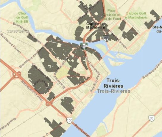
netic algorithm was used to optimize the cluster-               1. Number of generations: number of iterations
ing (using several techniques), we had to make some                on the fitness/breeding/mutation process.
choice according to the chosen clustering technique.
Since k-means algorithm was selected, the clustering            2. Chromosomes: Number of individuals config-
performance has been measured by the “Silhouette”                  urations tested by the process. Population.
metrics. This metric is documented by Kaufman and
                                                                3. Initial chromosomes initialisation:     The
Rousseeuw [19] and [17]. This metric includes two
                                                                   method used to initialize the chromosomes at
important equations. The distance between each
                                                                   generation 0.
point and the center of its cluster is shown in Eq.
2. The distance between the center of each cluster              4. Mutation rate: At breeding time, a percentage
is shown in Eq. 3. Finally, Eq. 5 uses the result of               of the chromosomes that do not inherits from
Eq. 3 and Eq. 4 to calculate the final "Silhouette                 parents but are randomly reinitialized.
score" that indicate the quality (the consistency) of
the clustering. The silhouette ranges from -1 to +1.            5. Percentage of chromosomes fitting well enough
Values from -1 to 0 indicates that the point is associ-            to breed: A threshold of the fitness func-
ated to a wrong cluster and from 0 to 1 are associated             tion. The chromosomes ranking better than
to a good cluster. The higher the value, the better                this value will be breeded in the next genera-
the cluster consistency [19].                                      tion.
                        1     X
                                                              The configuration maximizing the silhouette score
             a(i) =                d(i, j)          (3)
                    |ci − 1|                                  is displayed in Table 2 in the column "Best-Score",
                              j∈ci i6=j
                                                              where we maximized the Silhouette score using GA
                             1 X                              considering different number of clusters, number
              b(i) = min              d(i, j)       (4)
                       k6=i |ck |                             of features among the 8 features (Table 1). We
                                  j∈c
                                    k
                                                              reach a Silhouette score of 0.46, with N_init = 14,
                   b(i) − a(i)                                Max_iter = 196, 5 clusters using the features 1, 6,
         s(i) =                    , if |Ci | > 1   (5)
                  max (a(i), b(i))                            7, and 8. Otherwise, in some application cases, the
If most elements have a high value, then the clus-            number of clusters is fixed by the urbanism experts
tering configuration is appropriate. If many points           considering all features.
have a low or negative value, then the clustering con-
figuration may have too many or too few clusters. In          2.5    Feature-weighted inputs
our case, we had to create clusters of 5, 6, 7 or 8 di-
mensions. It is way more complicated to get a high            One important answer we had to find was the impor-
silhouette score than with some 2- or 3-dimensions            tance of each feature in the clustering process. To
features.                                                     do so, a loop evaluating the totality of the feature’s
                                                              list combination has been processed. This clustering
2.4    Genetic algoriths                                      process returned a silhouette score for each feature
                                                              combination. Having a list of features configuration
There are some relevant features to calculate a VI.           and silhouette index, the "random forest regressor"
Although, no label can be assigned to each set of fea-        technique was used to determine the importance of
tures. Therefore, we can not use a supervised learn-          each feature. A random forest is an iteration over n
ing algorithm. Unsupervised learning algorithms               "decision trees" (n = 250, in this case). The result
allow a machine to learn without labels, though.              was a list of importance ordered features and their
There are several techniques to do so, each one us-           weight.
ing some different parameters. Consequently, there
is a numerous of possible configurations. To opti-
                                                              2.6    Linear regression to predict VI
mize the results of the clustering, a GA (Cedeno,
1995) is used. Four genes are used in the evolution           The last stage of the proposed framework concerns
process: k-mean maximum iteration parameter, k-               the prediction of VI in the future for each first sur-
mean n centroid parameter, the number of clusters             rounding area districts. The VI were available by
to find, and a list of features. Table 2 shows the            dissemination area. There can be many dissemina-
configuration of the GA. The fitness function was             tion areas in each district. We had to regroup them
the silhouette score of the clustering. This metric           by district and calculate the linear regression line
that evaluate the cluster consistency is defined by           through the available years to predict 10 years later.
Eq. 4. The GA parameters are the following:                   Although, in some case, there is not many points

                                                          4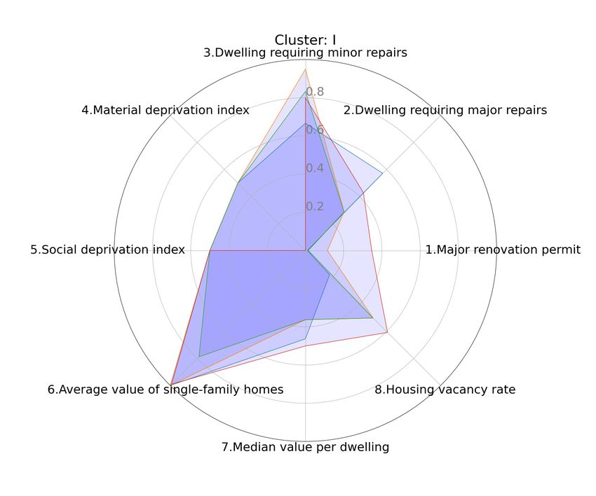
in the cloud, and it is hazardous to conclude to a              graphic issues (weak growth, aging of the popula-
reliable prediction.                                            tion, etc.). The city needed to have more infor-
                                                                mation about short-term vitality (5-10 years), aver-
                                                                age term vitality (10-20 years), and long-term vital-
3     Results applied on the                                    ity (20-30 years) of the first belt districts of Trois-
      first belt districts in Trois-                            Rivières. Basically, this study is focusing on this
                                                                vitality aspect. Many more aspects may be studied
      Rivières city                                             in some future work.

The Trois-Rivières territory as we know it exists
since an important fusion between six cities and mu-
                                                                3.1    Features distribution and repre-
nicipalities, in 2002. In this case, data from be-                     sentation
fore this fusion era is considered irrelevant. Trois-           First, let us see the distribution of each of the 8
Rivières aera is 334 km2 and has 136 000 people liv-            features for year 2016. There is a similar distribu-
ing on its territory. 40% of its territory is in agricul-       tion for each available year. Section 2.1 (Table 1)
tural area, 20% in rural area and 40% in urban area.            show to methodology to obtain these values. Fig. 4
It is situated at the junction of St-Laurent river and          shows the distribution of the features. The X-axis
St-Maurice river, about mid distance from Montreal              represent the dissemination area (DA) which is a ge-
and Quebec City. Trois-Rivières is also known for its           ographical location in the city. There is 135 of them
major infrastructures for planes, trains and ships.             in Trois-Rivières city. The Y-axis is the feature nor-
Fig. 2 shows a map of Trois-Rivières. The greyed                malized value. For each of the 135 dissemination
part is the first belt districts (the important part for        areas, and for every year, all the features are repre-
this study).                                                    sented on the same “radar” graphics. Since all fea-
                                                                tures are normalized, they can be displayed on the
                                                                same scale. Fig. 3 show an example of this radar
                                                                graphics (DA: 24370200 in year 2016).

                                                                3.2     Vitality index
                                                                In the graphics of Fig. 3, we can extract the aver-
                                                                age of the sum of the features. The result is also
                                                                a normalized value where a lower value means less
                                                                vitality and a higher value means more vitality.

Figure 2: The city of Trois-Rivières, Quebec,
Canada. The grey color defines the first belt area.

The urbanisation of its area happened in three steps.
The first one was prior to 1950. This area is called
“firsts districts” or “central districts”. The “first
belt” or “first agglomeration” was built between
1950 and 1980. Since then, the new areas are known
to be the “second belt” area. Since the important
fusion of 2002, residential development is more im-
portant than foreseen.                                          Figure 3: Typical "Radar" graphic used to represent
The city of Trois-Rivières needed to have some in-              the 8-dimensional features.
sights to write its urbanism plan. Specially, there
was a need to better foresee the vitality of the first
belt districts. The reason is that is some demo-

                                                            5
Feature 1       Feature 2

Feature 3       Feature 4

Feature 5       Feature 6

Feature 7       Feature 8

                            Figure 4: Features 1 to 8

            6
Although, this information is incomplete. There are
some very different district profiles having the same
average of the sum of the features. The best way
to visualise the district profile is to regroup them.
This was made by using the clustering technique de-
scribed in section 3.3 For this reason, this research
defines the vitality index by the two parts, as follow-
ing:
1. A letter representing the profile (cluster), and
2. A number representing the average of the sum
of the features. Figure 5: Clusters distribution histogram
For instance, "C45" means a "C" cluster with an av-
erage of the sum of the features of 0.45. The 45 value
is the average sum of the feature (0.45) multiplied
by 100. The inspiration of this classification sys-
tem comes from the works on star classification by
Annie-Jump Cannon in [7]. In this two-dimension
notation system, a star could have a G5 type.
Figure 6: Feature average for each dissemination
3.3 Clustering area, cluster division and cluster average
Like described in Section 3.3, the number of clus-
ters and the number of used features has been de-
termined by thousands of simulations of GA includ-
ing feedback analysis from urbanists. We were to
use all the 8 features and to divide the 135 aeras of
dissemination in 10 clusters. The distribution of the
clusters (year 2016) in shown in Fig. 5. For each
cluster on the X-axis, a distribution level on the Y-
axis. Fig. 6 shows on the Y-axis the average of the
sum of each feature (year 2016), for each dissemina-
tion area (X-axis). Vertical red lines divide the clus-
ters, and horizontal dotted lines show the average of
each cluster. The best way to visualize and interpret
every cluster is to superpose every radar graphic of
dissemination area of the same group. In Fig. 6, we
can see that the 6th and 7th (clusters F and G) have
about the same average of the sum of the features
(around 0.4). Without having their cluster profile, Figure 7: Cluster A and its stacked radar graphics
it would be impossible to see the difference.
Fig. 7 and Fig. 8 show the profile of those two It is even easier to see when both the profile and
clusters. We can easily see that even though they average of the sum of the features are different. Fig.
both have a similar average of the sum of the fea- 9 shows cluster I. Most of the cluster members are
tures, the distribution of theses sum values is not rather smalls.
the same. They have a very different profile.
7Figure 10: Silhouette metrics using 4 features: a) 5
clusters b) 10 clusters (2016 data).
Fig. 11 shows the typical evolution of fitness func-
tion of GA defined by the Silhouette score. Red
curve represents the silhouette score average and
green curve represents the silhouette score maxi-
mum.
Figure 8: Cluster H and its stacked radar graphics
Table 2: Chromosome clustering configuration max-
imizing the Silhouette score (Best-Cluster) and spec-
ifying the number of cluster (Fixed-Cluster).
Figure 9: Cluster I and its stacked radar graphics
Fig. 3a shows the distribution of the features be-
tween 5 clusters. We can note that there are very
few clustering errors (from -1 to 0) and a silhouette
score value of 0.46. This is the configuration that
optimizes the silhouette score. Fig. 3b shows the
distribution of the features between 10 clusters. We
Figure 11: Typical evolution of silhouette score over
can note that there are very few clustering errors
generations.
(from -1 to 0) and a silhouette score value of 0.22.
As mentioned earlier, the clustering process was op-
timized by a GA. The results shown in Table 2 for 10
clusters given Silhouette score of 0.22. The N_ init 3.4 Weighting the features
parameter is the number of times the k-means algo-
Urbanists wanted to know which features are the
rithm will be run with different centroid seeds. The
most relevant in the clustering process. Section 2.5
Max iter is the maximum number of iterations of the
presented a methodology based on a Random For-
k-means algorithm for a single run.
est algorithm to weight the 8 features proposed by
urbanists. The weights of the features in 2016 are
given by Fig. 12. In order of importance, from the
8most important to the least important (the number such a prediction using past VI (numeric part) com-
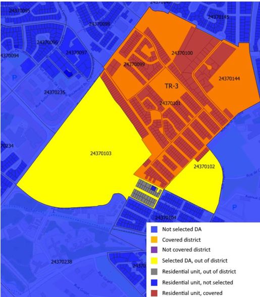
in parenthesis is the level of importance): puted on 6 areas of dissemination (on 3 years 2006,
2011 and 2016). Each aera of dissemination is de-
1. feature 3 (0.125) Proportion of dwelling requir- fined by a blue dot. In this case, the 6 areas are those
ing minor repairs included in the TR-3 district. Those results are some
examples taken in the final report [10] written for ur-
2. feature 2 (0.122363) Proportion of dwelling re- banists of the city of Trois-Rivières. Obviously, this
quiring major repairs report includes hundreds of figures to illustrate data
3. feature 8 (0.113767) Housing vacancy rate on every district of the first belt and every dissemi-
nation area.
4. feature 6 (0.112084) Average value of single-
family homes
5. feature 5 (0.109790) Social deprivation index
6. feature 4 (0.109603) Material deprivation in-
dex
7. feature 7 (0.109569) Median value per dwelling
8. feature 1 (0.109211) Major renovation permit
Figure 13: Map of TR-3 district of Trois-Rivières
and its dissemination areas.
Figure 12: Weights of feature.
3.5 Predicting vitality indexes
This research is only able to predict the average of
the sum of the features part of the VI. At least for
the numeric part it is possible to have a regression
that learns from the past to estimate future. Since
the goal is to predict vitality in the first surround-
ing area, we have first to regroup dissemination area.
Fig. 13 shows a district that includes four areas of
dissemination. It is usually from 1 to 7 per district.
To make some prediction, we must plot the VI (nu- Figure 14: Regression line and vitality prediction
meric part) of each aera of dissemination included in based on areas of dissemination of the past, for TR-
each district. Then the regression line must be added 6 district of TroisRivières city.
and used to make the prediction about the future.
In this case, results must be interpreted with caution
since there are only three years of history to predict
years 2021 and 2026. Fig. 14 shows an example of
94 Discussions than a model based on a crispy clustering algorithm.
Some improvement can also be done by making some
A method for calculating and predicting a VI has prediction on each available feature, instead of only
been developed in this paper. The main objective the numeric part of the VI (which is the average of
was to help urbanists to have a better understand- those features). Since this system must deal with
ing of the raw data available in different sources, an input that includes multiple features, some algo-
including their own. The data was collected, then rithms based on dimensionality reduction must be
pre-processed to optimize distribution and readabil- explored. There could be some improvement possi-
ity. Four ML algorithms were used to process data: bilities by using this solution in the pro-processing
k-mean clustering technique, GA, feature-weighted phase. Finally, in a next version, it will be easy
inputs and linear regression. There is no simple way to also project the profile part of the VI. It will be
to use a GA on some clustering techniques. For certainly possible to predict the shapes of the mul-
different clustering techniques, we must use differ- tidimension VI of the future.
ent types of parameters. There are also some issues
about the evaluation of the results of the clustering.
The Silhouette metrics finally did a fair job to evalu- 6 Acknowledment
ate the clusters consistency. Obviously, the cluster-
ing of some 8-dimensions indexes is a greater chal- This work has been supported by the City of Trois-
lenge than the 2- dimensions points cloud clusters Rivières, The "Cellule d’expertise en robotique et in-
usually presented. Due to this higher dimensionality, telligence artificielle" of the Cégep de Trois-Rivières
there was also some issues about the graphical repre- and IDE Trois-Rivières.
sentation of the features. The “radar” graphic type
was very useful. The new custom “Omni” graphic
type invented for the purpose was also helpful to
References
present the totality of the information at a glimpse. [1] Ida vitality index.
The superposed radar graphic was also helpful to
visualize the clusters consistency, maybe in an even [2] There goes the neighborhood: New hope
better way than using the Silhouette metric. The are emerges in one of the city’s roughest areas.
some tables of appreciation of the Silhouette scores,
[3] Jamal Abed and Isam Kaysi. Identifying ur-
but they are based on some 2- dimensions features.
ban boundaries: application of remote sensing
It is very difficult to know if some 8- dimensions
and geographic information system technolo-
features clusters (like the ones in this research) are
gies. Canadian Journal of Civil Engineering,
consistent or not. That is why the superposition of
30(6):992–999, 2003.
the radar graphics was so important to confirm the
clusters consistency. At the end, this research suc- [4] Donald Appleyard. Styles and methods of struc-
ceeds in converting some scattered raw data in some turing a city. 2(1):100–117. Place: US Pub-
valuable knowledge, well presented and useful for the lisher: Sage Publications.
writing of the urban plan of Trois-Rivières city.
[5] Nikolay Arefiev, Vitaly Terleev, and Vladimir
Badenko. GIS-based fuzzy method for urban
5 Conclusion planning. 117:39–44.
All the code written in this research has some great [6] Christopher Charles Benninger. Principles of
generalization perspectives. In a near future, it intelligent urbanism: The case of the new capi-
could be converted in a more general urban tool to tal plan for bhutan. 69(412):pp. 60–80.
make some prediction about a broader range of ur- [7] Annie Jump Cannon. Classification of 1477
ban indexes, such as criminality indexes, health in- stars by means of their photographic spectra.
dexes or economic indexes. There are also some im- Harvard Obs. Annals, 56:65–114, 1912.
provement possibilities in the clustering part. The
clustering method and the metrics could be studied [8] B. Cheng, Salvatore Longo, F. Cirillo,
and improve. One way of improving a next version M. Bauer, and E. Kovacs. Building a big
would be to replace the k-mean clustering algorithm data platform for smart cities: Experience and
by a c-mean algorithm. This would have the benefits lessons from santander. 2015 IEEE Interna-
of fuzzifying the districts limits. A model based on tional Congress on Big Data, pages 592–599,
fuzzy clustering would reflect reality in a better way 2015.
10[9] KEITH C. CLARKE and LEONARD J. GAY- [19] Leonard Kaufman and Peter Rousseeuw. Find-
DOS. Loose-coupling a cellular automa- ing Groups in Data: An Introduction to Cluster
ton model and gis: long-term urban growth Analysis. 09 2009.
prediction for san francisco and washing-
ton/baltimore. International Journal of Geo- [20] Verda Kocabas and Suzana Dragicevic.
graphical Information Science, 12(7):699–714, Bayesian networks and agent-based modeling
1998. PMID: 12294536. approach for urban land-use and population
density change: a BNAS model. Journal of
[10] & Simard J. Dessureault JS., Massicotte D. Geographical Systems, 15(4):403–426, October
Rapport final Ville de Trois-Rivières – Prévi- 2013.
sion de la vitalité des secteurs de la première
couronne de Trois-Rivières. Trois-Rivières. [21] Benjamin Kuipers. Modeling spatial knowledge.
Technical report, 2019. 2(2):129–153.
[11] J. E. Drewes and M. van Aswegen. Determining [22] Xia Li and Anthony Gar-On Yeh. Neural-
the vitality of urban centres. pages 15–25. network-based cellular automata for simulating
multiple land use changes using gis. Interna-
[12] Shan Feng and Lida Xu. An intelligent decision tional Journal of Geographical Information Sci-
support system for fuzzy comprehensive evalu- ence, 16(4):323–343, 2002.
ation of urban development. 16(1):21 – 32.
[23] Yi Liu, Xuesong Feng, Quan Wang, Hemeizi
[13] E. Foroutan, M. R. Delavar, and B. N. Araabi. Zhang, and Xinye Wang. Prediction of urban
Integration of Genetic Algorithms and Fuzzy road congestion using a bayesian network ap-
Logic for Urban Growth Modeling. ISPRS An- proach. page 8.
nals of Photogrammetry, Remote Sensing and
Spatial Information Sciences, I2:69–74, July [24] Arun Mahizhnan. Smart cities: The singapore
2012. case. 16(1):13 – 18.
[14] Nikolas Geroliminis, Konstantinos Kepapt- [25] Phillip C. Muehrcke. Cartography and geo-
soglou, and Matthew Karlaftis. A hybrid hy- graphic information systems. Cartography and
percube – genetic algorithm approach for de- Geographic Information Systems, 17(1):7–15,
ploying many emergency response mobile units 1990.
in an urban network. European Journal of Op-
erational Research, 210:287–300, 04 2011. [26] Beniamino Murgante, Giuseppe Borruso, and
Alessandra Lapucci. Geocomputation and
[15] George Grekousis, Panos Manetos, and Yor- urban planning. In Beniamino Murgante,
gos N. Photis. Modeling urban evolution using Giuseppe Borruso, and Alessandra Lapucci,
neural networks, fuzzy logic and GIS: The case editors, Geocomputation and Urban Planning,
of the athens metropolitan area. 30:193–203. pages 1–17. Springer Berlin Heidelberg.
[16] Qingfeng Guan, Liming Wang, and Keith C. [27] B.C Pijanowski, A. Tayyebi, M.R. Delavar, and
Clarke. An artificial-neural-network-based, con- M.J. Yazdanpanah. Urban expansion simula-
strained ca model for simulating urban growth. tion using geospatial information system and
Cartography and Geographic Information Sci- artificial neural networks. International Journal
ence, 32(4):369–380, 2005. of Environmental Research, 3(4):493–502, 2009.
[17] Natacha Gueorguieva, Iren Valova, and George [28] Andreas Rienow and Dirk Stenger. Geosimula-
Georgiev. M&MFCM: Fuzzy c-means cluster- tion of urban growth and demographic decline
ing with mahalanobis and minkowski distance in the Ruhr: a case study for 2025 using the ar-
metrics. 114:224–233. tificial intelligence of cells and agents. Journal
of Geographical Systems, 16(3):311–342, July
[18] Yufang Hao and Shaodong Xie. Optimal re- 2014.
distribution of an urban air quality monitor-
ing network using atmospheric dispersion model [29] Stephanie Santoso and Andreas Kuehn. Intelli-
and genetic algorithm. Atmospheric Environ- gent urbanism: Convivial living in smart cities.
ment, 177:222–233, March 2018. page 5.
11[30] Alì Soltani and Davoud Karimzadeh. The [34] L. . X. Wang and J. M. Mendel. Fuzzy basis
spatio-temporal modeling of urban growth us- functions, universal approximation, and orthog-
ing remote sensing and intelligent algorithms, onal least-squares learning. IEEE Transactions
case of mahabad, iran. 6(2):189–200. on Neural Networks, 3(5):807–814, 1992.
[31] Saber Talari, Miadreza Shafie-khah, Pierluigi
Siano, Vincenzo Loia, Aurelio Tommasetti, and [35] Ning Wu and Elisabete A. Silva. Artificial
João P. S. Catalão. A review of smart cities intelligence solutions for urban land dynam-
based on the internet of things concept. Ener- ics: A review. Journal of Planning Literature,
gies, 10(4), 2017. 24(3):246–265, 2010.
[32] Amin Tayyebi, Bryan Pijanowski, and
Amir Hossein Tayyebi. An urban growth [36] X. Yang, R. Chen, and X.Q. Zheng. Simulat-
boundary model using neural networks, gis ing land use change by integrating ann-ca model
and radial parameterization: An application to and landscape pattern indices. Geomatics, Nat-
tehran, iran. Landscape and Urban Planning, ural Hazards and Risk, 7(3):918–932, 2016.
100:35–44, 03 2011.
[33] Ziyu Tong. A genetic algorithm approach to [37] Kapetanakis K. Zampoglou M., Malamos A.
optimizing the distribution of buildings in ur- Big data and internet of things: A roadmap
ban green space. Automation in Construction, for smart environments. Springer International
72(P1):46–51, 2016. Publishing, 2014.
12You can also read