Probing dark matter large scale structure: convergence mapping via galaxy weak lensing and cross-correlations with CMB weak lensing
←
→
Page content transcription
If your browser does not render page correctly, please read the page content below
Probing dark matter large scale structure:
 convergence mapping via galaxy weak lensing and
     cross-correlations with CMB weak lensing

                            Charlotte Welker
                               April-July 2011

Summary: In this project we reconstruct and test an unusually large convergence
map using galaxy weak lensing data from the CFHT in linear approximation. We
then cross-correlate them with CMB lensing data from ACT project, and cluster
maps to increase resolution and explore new methods to study the growth of
structure in the universe

keywords: dark matter, weak lensing, CMB, cross-correlations, convergence, ACT,
CFHT

Cosmology group , Lawrence Berkeley National Laboratory,
Berkeley , California , USA
under supervision of: Pr. Eric Linder, Dr. Alexie Leauthaud and Dr.
Sudeep Das. (evlinder@lbl.gov)

M2 Physique Fondamentale
Ecole Normale Superieure de Lyon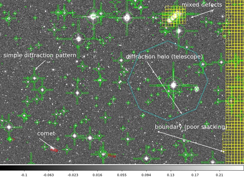
Contents

Introduction                                                                                                                     2

1    Theory and description of the project                                                                                       3
    1.1 weak gravitational lensing and dark matter . . . . . . . . . . . . . . . . . .                                           3
    1.2 The CFHT Stripe82 survey . . . . . . . . . . . . . . . . . . . . . . . . . . .                                           4
    1.3 Overview of CMB Lensing and Cross-correlations with ACT maps . . . . .                                                   6

2 From the telescope to the convergence map                                                                                      7
  2.1 Pre-processing: images and data extraction .          .   .   .   .   .   .   .   .   .   .   .   .   .   .   .   .   .    7
  2.2 Reconstruction of the large convergence map           .   .   .   .   .   .   .   .   .   .   .   .   .   .   .   .   .    8
  2.3 Tests . . . . . . . . . . . . . . . . . . . . . . .   .   .   .   .   .   .   .   .   .   .   .   .   .   .   .   .   .   11
      2.3.1 kappa distribution and noise . . . . .          .   .   .   .   .   .   .   .   .   .   .   .   .   .   .   .   .   11
      2.3.2 B-modes and systematics . . . . . . .           .   .   .   .   .   .   .   .   .   .   .   .   .   .   .   .   .   11
      2.3.3 cluster detection . . . . . . . . . . . .       .   .   .   .   .   .   .   .   .   .   .   .   .   .   .   .   .   12

3 Real space cross-correlations                                                                                                 15
  3.1 cluster maps: cs82 and CMB . . . . . . . . . . . . . . . . . . . . . . . . . .                                            15
  3.2 Cross-correlations with ACT maps . . . . . . . . . . . . . . . . . . . . . . .                                            16
  3.3 Fourier space cross-correlations: Prospects . . . . . . . . . . . . . . . . . . .                                         18

Conclusion                                                                                                                      20

Acknowledgements                                                                                                                21

A General pipeline.                                                                                                             24

B kernels in weak lensing                                                                                                       26

C   Mask processing                                                                                                             28

D Example of maps built from cs82 catalog data                                                                                  30

E cs82 κ map with positions of known clusters in this area.                                                                     32

F Stripe82 Layout                                                                                                               34

G Real space cross-correlations                                                                                                 36

H ACT maps                                                                                                                      38

                                              1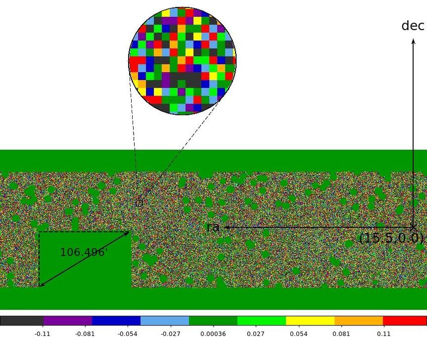
Introduction

Dark matter is matter that neither emits nor scatters any electromagnetic radiation,
rendering direct observation impossible. Nonetheless, it is currently thought to represent
83 % of all the matter in the universe and to account for most of galaxy properties and
structure formation. That is why it has become both a theoretical stake and an observational
challenge to find evidence of its presence and to understand its structure.
    The recent urge to track this "invisible" portion of the matter relies on modern astron-
omy’s ability to resolve its indirect gravitational effects on the visible structures, in this
particular project its gravitational lensing effects on background galaxy clusters and Cosmic
Microwave Background (CMB) anisotropies. Indeed, the mass of a local patch of dark
matter will bend the trajectory of light beams that pass nearby resulting in the distortion
of their images observed through telescopes. By analyzing those distortions, we are able to
infer the distribution of dark matter on the projected sky.
    The project described here aims to investigate those possibilities and improve our
knowledge of dark matter large scale structure, using and testing new promising methods,
notably the possibility to cross-correlate data extracted from both types of sources to
increase the precision. Thus, in a first part, we will expose the underlying theory, along
with an overview of the surveys involved in this study with their specificities. Then, in a
second part, we will develop the mapping part of the project: the reconstruction of the
largest dark matter distribution map ever deduced from galaxy lensing. And eventually, in
the last part we will focus on the pilot study of cross-correlations with CMB lensing data
and stress their potential interest for further studies.

                                              2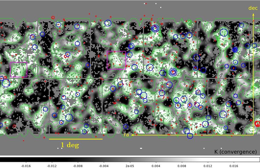
Chapter 1

Theory and description of the
project

1.1     weak gravitational lensing and dark matter
  As explained in introduction, gravitational lensing is an effect of the curvature of the
time-space in general relativity. The newtonian potential φ that appears in the metric
causes the light beams passing by a massive object to get deviated from their straight line
trajectory, resulting in a distortion of the image we can see of their source.

thin lens approximation, weak galaxy lensing and linear theory of conver-
gence reconstruction
Providing that the distribution of massive "lenses" has a small depth compared to its distance
to the source and to the telescope, this effect is similar to having a thin lens on the path of
the light between the source and the telescope, hence its name.(See B ) For small deflections,
in the linear approximation, the deflection includes only gradient terms of the potential
and the lensing corresponds to a remapping of the projected image of the sources. We can
define a deformation matrix to change actual coordinates β~ into lensed ones θ.   ~

                           ∂ β~
                                                              !
                                     1 − κ − γ1    −γ2
                                =                                                         (1.1)
                           ∂ θ~         −γ2     1 − κ + γ1
    where γ1 and γ2 can be seen as the two components of a vector ~γ that characterizes the
shear, or shape distortion, while κ is called the convergence.( For further details see [1], [5]
and [4]).
    Then, as dark matter is the dominant (in mass) term along the line of sight, mapping
convergence reveals to be a very accurate way to map the projected dark matter mass
distribution. As described in details in [2],[3] and [5], the observed shear and the convergence
are related to the gravitational potential Ψ of the lenses by:

                        1                               1
                  γ1 = (∂12 − ∂22 )Ψ γ2 = ∂1 ∂2 .Ψ κ = (∂12 + ∂22 )Ψ                 (1.2)
                        2                               2
    It can be proved that convergence and Σ, the projected map along the line of sight are
related by: κ = ΣΣ(θ)
                  crit
                       with:
                                             c2    Ds
                                    Σcrit =      .                                   (1.3)
                                            4πG Dl .Dls

                                               3
where G is Newton’s constant, c is the speed of light and Ds , Dl and Dls are the
angular-diameter distances between the observer and the galaxies, the observer and the lens,
and the lens and the galaxies. We notice that Σcrit varies with redshift. The reconstruction
method then take the kernel into account to renormalize κ properly.
   Then the Fourier transforms (hatted letters) of γ1 and γ2 writes, for i = 1, 2:

                                                                   γ̂i = P̂i .κ̂          (1.4)
                                       p21   −    p22                  2p1 p2
                           Pˆ1 (~
                                p) =                        Pˆ2 (~
                                                                 p) =                     (1.5)
                                             p2                          p2

    with Pˆ1 (~
              p) = 0 when p21 = p22 and Pˆ2 (~
                                             p) = 0 when p1 = 0 or p2 = 0
    κ̂ and κ can then be reconstructed. Practically, a noise component is added to γ̂i ,then κ
is reconstructed using a least mean square estimator:

                                       κ
                                       b=P
                                         c1 .γ
                                             c1 + P
                                                  c2 γ
                                                     c2                                   (1.6)

units used in the study
In this project, as we are observing projections of the area recorded on a 2D spherical surface,
we use equatorial angular coordinates: RA and dec, to locate a point on this projection.
    Due to local defects of the telescope, those coordinates are not merely spherical but must
be adjusted by interpolation procedures to match precisely known bright star positions.
This fitting procedure is referred to as astrometry and can be a great source of errors if not
optimized.
    To characterize the depth of the area recorded on the telescope, we use for convenience
the redshift z, which is not a linear measure of comoving distance but is directly measured
from spectrum for every object observed.

1.2     The CFHT Stripe82 survey
  To achieve the convergence reconstruction, observational data were collected via the Stripe
82 survey ("cs82", complete description available online, see [9]), using the Canada-France-
Hawai-Telescope (CFHT). The set up and the way sky maps are recorded is described here
below.

experimental set up
   The stripe 82 survey consists in a series of overlapping pointings (each one covering one
square degree), spanning a total of 2 degrees in dec and 82 degrees in RA, with a 0.2 arcsec
pixel. It probes the sky to a depth of roughly z = 0.8 in redshift. Optimization procedures
include shifts of the telescope when a too bright star is saturating the image, so as to
maximize the usable surface of measurement. A sketch of the resulting layout can be found
in Appendix F.
    The photon count images (corrected from cosmic rays and optical distorsions, notably
via stacking, which might result in lower resolution close to the edges) are the primary maps
for this study.

                                                        4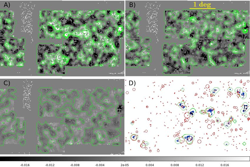
Figure 1.1: example of elliptic fit

Observations: approximations and limitations
   Then, the weak lensing processing of those maps requires the construction of source
catalogs and shape detection.
    First, the sources are extracted with the software Sextractor (designed by Emmanuel
Bertin, see [10]), with respect to a chosen signal over noise threshold and their coordinates,
size and magnitude are stored in a catalog. They’re also sorted as galaxy, star or comet,
which is used to "mask" the catalog: the information concerning stars or comets is deleted.
    In order to proceed to the weak lensing study, galaxy redshift and shear values need to
be extracted too.
    In this survey, we can see the dark matter we are tracking as a lens because its distribution
is not uniform but shows a peak at z = 0.2 and vanishes with a standard deviation of ∆z 0.2
around this value.
    The existence of this kernel is directly related to the kernel of the sources, which is itself
the result of limitation in volume at low z for a fixed solid angle, and optical limitation in
brightness at high z. An illustration can be found in Appendix B.
    As for the redshift, given the huge number of galaxies considered, a fast photometric
method using a set of 5 wavelength filters distributed over a wide scale so as to infer the
position of the theoretical break (static: 4000Ao ) is preferred to a full spectrum recording.
The redshift is then known to a relative precision of ∆z  z = 0.1.
    As for the shape shear, we proceed as shown figure 1.1. We make the assumption that
every galaxy detected is on average truly spherical, then elliptically distorted by the linear
lensing. The bright area is then fitted as precisely as possible to an ellipse, and shear is
deduced linearly from ellipticity. Indeed, In the absence of observational distortions, the
                                                                                   eint +γ
observed ellipticity eobs is related to its unlensed value eint through: eobs = 1+γ   ∗ .eint
    This approximation might seem very rough but it becomes relevant if the shear is
averaged over enough galaxies, which means that the map pixelization needs to be degraded
as we will see in part 2.
    Main remaining sources of errors come from the point spread function (psf) correction:
due to atmosphere scattering as well as noise in from the apparatus, a point-like source
appears as a patch. Correction via analysis of star psf might be locally approximative.

                                                5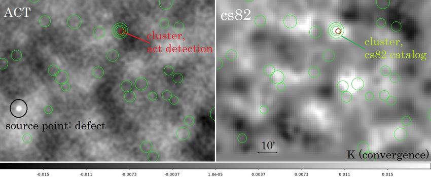
Then again, a reasonable averaging along with the fact that the final map is a convergence
map, which is not a completely local measurement solves most of the problem. For that
purpose, every galaxy is assigned a weight which characterizes its relevancy in the sample.
This weight ω is defined as ω = σ12 where σ is the error over average for each patch of pixels
corresponding to a galaxy.

1.3     Overview of CMB Lensing and Cross-correlations with
        ACT maps
The Cosmic Microwave Background, or CMB, is the relic radiation that we perceive from
the photon decoupling epoch when the universe became transparent. Because this phase
happened over a very short amount of time compared to others in early universe evolution,
CMB can be approximated by a 2D sheet-like very homogeneous source at z = 1100(see [6]
for more information) with statistically Gaussian fluctuations.
    In the linear range, CMB lensing corresponds to a remapping and is sensitive to variations
δMdark of dark matter over the patch we are observing.
    Just like galaxies, CMB also has a lensing kernel that peaks around z = 1 − 3. (as shown
on figure B in Appendix). In this study, we worked with patches from the ACT survey
(Atacama Cosmology Telescope, see [11]), which records CMB temperature maps, infering
unlensed CMB and then convergence maps. As this kernel is overlapping with the cs82
galaxy lensing one, we can expect to see a clear cross-correlation signal, which could help:

   • improve the precision of κ maps, as both surveys have different sources of noise and
     systematics

   • to infer distance ratios and then undertake tomography studies to unravel dark matter
     distribution in redshift, i.e. reconstruct its the evolution and compare it to growth of
     structure models ( methods and models described in [7] and [8].)

   • constraint cosmological constants and refine models by comparing the cross-power
     spectrum to the theory.

     Indeed, the mapped 2D signals on the sky can be developed into spherical harmonics
~l, m (rather than in common Fourier modes) . For θ the position on the projected sky, be
 T (θ) the intrinsic temperature of the CMB and ∆T  (θ)
                                                 T (θ) its fluctuations. Then we define:

                          ∞ X l
                ∆T (θ) X
                       =          alm Ylm (θ, φ) and         Cl = h|alm |2 im,stat                   (1.7)
                 T (θ)   l=0 m=−l

    Graphs (Cl , l) can be fitted and compared to theory, and we can as well define cross-
correlation coefficients in ~l space from ACT and cs82 κ maps, with W the weights (lens
                                                                cdt
kernels), g the galaxy source kernel, δ the densities, and dη = a(t) the comoving distance
variation as:

                                                         κ    κCM B           B∗ gal
                                                     Cl gal              b CM
                                                                      = hκ lm   b lm iensemble
                                                                                κ                    (1.8)
                Z                                        Z
      κCM B =            dηδ(η)WCM B (η, η0 )   κgal =           dη 0 dηδ(η)g(η 0 , ηWgal (η, η0 )   (1.9)
                 depth                                   depth

                                                 6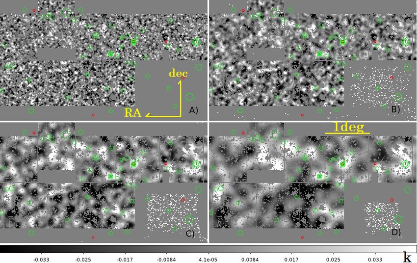
Chapter 2

From the telescope to the
convergence map

  We are now going to focus on the reconstruction of the convergence map itself. Considering
the width of our patch, our goal is mostly to probe the large scale structure of the dark
matter distribution. The overall pipeline of the project is presented in Appendix A.

2.1     Pre-processing: images and data extraction
Recombination and astrometry
  First, the individual square patches have to be recombined into a large stripe, and that is
where the importance of overlapping becomes obvious: because of the stacking, the edges
tend to have lower resolution than the middle of the map. However, by combining two
contiguous patches we can select the best record for each structure. We can also get rid of
some diffraction patterns without losing information.
    This phase was carried out writing IDL programs. We used the astrometry information
(RA,dec) to create a large template and match objects in overlaps (using distance thresholds
varying with size of structure), then average their position,and build a large catalogue. A
better astrometry leads to better results. With the actual astrometry deviation of a few
arcseconds is still detected in some cases for the same object in two different patches. The
combining allows at least to uniformize the astrometry over the stripe.

Masks
   Stars as well as comets can generate oblong shapes due to telescope diffraction or exposure
duration, and introduce huge errors when interpreted as distorted background galaxies.
Thus it is absolutely necessary to mask them.Those areas, which don’t contain weak lensing
information will then be left blank in our final convergence map.
    Then, in order to create those masks, programs start from the images. The unwanted
objects are flagged based on shape, redshift and magnitude criteria as shown on figure 2.1
and specifically shaped masks are designed for each type of defect. This step was carried
out for separate pointings by Pr. Ludovic Van Waerbeke (University of British Columbia)
prior to this internship.

 The main idea was then to convert these data in a properly pixelized full stripe mask
map adapted to the final convergence map we want to get.

                                              7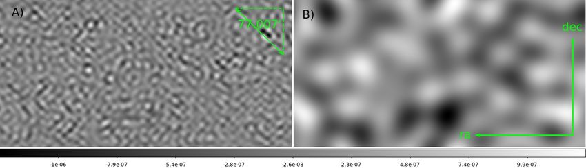
Figure 2.1: pre-mask: detection and sorting of parasite structures
                  different colors correspond to different purpose masks

Averaging and repixelisation
   Indeed, as emphasized in Part 1, the shear (γ1 , γ2 ) need to be averaged over a sufficient
number of galaxies, 10 being a generally approved minimum.
    Because this map is aimed to be used in cross-correlation with other maps, we chose
a standard scale of one square arcmin pixel, which corresponds to an average of 7.6+     − 0.1
galaxies per pixel,values ranging from 0 to 30 in the heaviest clusters.(It must be noticed
that an average cluster of 10 arcmin width is divided in roughly 100 pixels) Then, a full
stripe template was created and the shear data from the catalog were sorted with respect
to their position and averaged into pixels, weights being taken into account, to create γ
maps as shown in Appendix D.(codes written with IDL)
    This entails a certain number of approximations, especially because masks need to
be repixelized on the same template. Appendix C shows how we proceeded to the pixel
discrimination and lists the errors we may have introduced. Figure 2.2 illustrates the overall
process.

2.2     Reconstruction of the large convergence map
Method and first maps
The actual κ map, or the dark matter projected 2D map, can now be reconstructed from
the γ maps (1 and 2), the mask map, and a galaxy density map counting the number of
objects in each pixel.
    These data are used as inputs in a Fortran90 code designed and optimized by Pr. Ludovic
Van Waerbeke (University of British Columbia), that deduces the κ map using Fourier
transform (assuming all the distortions remain in the linear range), as described in Part 1.
    This code offers the possibility to smooth the map over a chosen number of pixels for
radius, with a chosen function. A Gaussian smoothing appeared to be the best option as
it was closer to the dispersion function of structures on telescope records, and as we were

                                              8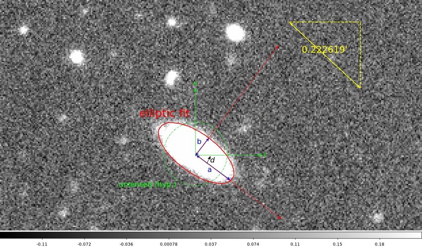
Figure 2.2: Shear averaging: map with pixel size and errors a priori
                     blue box: unmasked pixel, red box: masked pixel

reconstructing convergence map on a patch much wider than any correlation length.
    Resulting maps with various smoothing are shown on Figure 2.3.

optimization of smoothing and masking
As can be seen on map A), a too small smoothing is unable to unravel the large scale
structure because it gives equal spatial importance to noise and actual convergence detection.
    As the smoothing increases, giving better visibility to convergence peaks, the structure
slowly emerges from the noise revealing a filamentary structure that should follow the
projected cluster distribution as dark matter is expected to reach high density in those
objects (hence local over-densities account for their formation).
    A too wide smoothing though tends to create large scale correlations that do not
correspond to any physical reality, which blurs the map.
    To optimize the smoothing, we fitted the width of the peaks with the radius of heavy
clusters we found at the same positions. For that purpose, we created cluster maps out
of cluster catalogs, built with the same detection procedure as for galaxy catalog except
with a higher signal
               noise threshold. (lensing detection 6σ i.e. structures with shear higher than
mean + 6 standard deviation in the overall distribution.)
    We focused on heaviest clusters (over 100 galaxies), around most relevant redshift for
our detection (peak of the kernel: z = 0.4). They have an angular size of 10+      − 1 arcmin,
which, given the redshift, corresponds to an actual size of ∼ 3 Mpc. Map C) smoothing
is optimized: the size of those clusters is preserved as well as the visibility of large scale
structure. This latter effect can be checked on Figure E.1 where lower richness or mass
structures are superimposed on the map and follow the light grey distribution with great
accuracy.

                                              9
Figure 2.3: patch from S82p convergence (κ) map with Gaussian smoothing:
A) σ = 1 pix., B) σ = 2 pix., C) σ = 4 pix., D) σ = 7 pix. green: cs82 high richness (> 20)
clusters (to scale) in redshift range [0.15, 0.6] . richness > 100: 3-circled; red: ACT detected
clusters
102.3 Tests
2.3.1 kappa distribution and noise
Before proceeding to the cross-correlations, we needed to test the accuracy of the κ map.
As a first test, we plotted the κ distribution function, (extracted with an IDL code
1
sorting κ values with a precision of 500 of the total map range): for the final map, for
a gaussianly randomized γ map, and finally for κ values located at the same position as
clusters(meaning located within its recorded boundaries) exclusively. Those latter maps
were generated writing IDL codes.
Generally speaking, a randomized map is a good estimate of the level of noise we can
expect as a result of the overall processing and especially the reconstruction step. As can
be seen in figure 2.5, the values from the noise (map C) ) are clearly lower than the actual
reconstructed κ values (map A) ). The general signal
noise ratio is ranging from 5 to 10 depending
on the patch we consider, which tends to prove the reasonable quality of our signal.
One may notice that the average κ values we get are, in general, smaller by a factor 6 to
10 than values that can be found in smaller scale smoothed weak lensing studies (see [12]).
Remembering that our map features a projected distribution of all the dark matter
lensing along the line of sight, this should be understood as a result of both the limited
redshift depth of the survey and the averaging procedure: As this survey records data on a
unusually large stripe (160 deg2 ) but with shorter mean exposure duration, we are probing
weak lensing sources in a thinner kernel (z = 0.7 − 0.9) than most of other studies, resulting
in a thinner dark matter detection kernel (z = 0.3 − 0.5).
As for the distribution of κ around known rich clusters, we noticed a clear shift of the
overall distribution. The mean for the whole map being κ = 0.00036+ − 5% while it goes up
+
to κ = 0.0045− 5% around clusters (top peak values: 0.01 to 0.03). The distribution is also
skewed towards the positive values: the (+,-) ratio goes from (0.51,0.49) up to (0.68,0.32)
as expected due to the non-random aspect of this selection.
2.3.2 B-modes and systematics
If the previous tests confirmed that we had reconstructed an actual convergence map, they
are unable reveal possible local fake positives due to systematics in measurements.
In order to investigate this aspect, we needed to compare our map to the B-mode map.
Indeed, as shown on Figure 2.4, our reconstruction is based on the idea that linear weak
lensing induces only distortions tangential to the lens distribution, or E-modes (curl terms
are a second order correction). Then, if systematics exist they will be easily detected in
orthogonal B-modes that are not generated otherwise.
To estimate the influence of those errors on our map, we flipped those modes around
by 45 deg to reconstruct a κ map using the same code. It is mathematically equivalent to
change (γ1 , γ2 ) in (γ1B , γ2B ) according to:
γ1 = γ. cos(2θ) γ2 = γ. sin(2θ) (2.1)
π π
γ1B = γ. cos(2(θ + )) γ2B = γ. sin(2(θ + ))
4 4
γ1B = γ2 γ2B = −γ1 (2.2)
The B-mode map is shown in Figure 2.5 (B). It is easy to notice that the level of B-modes
is high even though smaller than on average than the actual signal. The ratio B E can reach
0.6 in object rich areas, which results in existence of fake positive in our final map.
11Figure 2.4: Description of different modes
The reconstruction code is optimized to take the edges of the window and the mask into
account in the Fourier transform and minimize harmonic peaks. A gaussian apodisation
(guaussian smoothing of the edges) was performed and showed no difference in intensity or
distribution of peaks over the map. Then, most probable origins for those systematics are
errors in the PSF correction and the astrometry. the PSF corrections being optimized in
our case, the best candidate to explain those defects is the astrometry interpolation, which
still need to be improved.
2.3.3 cluster detection
Because of the presence of B-modes it it important to check with cluster and galaxy maps
that we are detecting the large scale structure properly, which can be seen in Appendix,
on Figure E.1, where the voids remain free from clusters, which on the contrary pack on
dark matter high density areas. If high richness cluster match the peaks, medium richness
or low redshift clusters and galaxies follow the structure. Nevertheless, we can see some
unexplained high densities which reveal the existence of those B-mode type fake positives.
However, performing a structure detection (IDL) with respect to signal
noise , we can see that
(Figure 2.6 ), providing that we set a proper threshold (here 5.0) for this ratio, we detect
many more (and much more clearly) structures with the actual κ map than with the B-mode
map.
It is also perfectly normal that not all the clusters are detected as one may notice that:
• The map is partially masked in a complex way
• This cluster map spans a redshift range of z = [0.15, 0.6] while the detection kernel is
centered on z = 0.4
• The clusters are mapped with respect to a lensing kernel too, so that a "large" cluster
might be well located and reasonably massive (=proper lens) but it could also be
massive but too close, or massive but far closer to the sources than to the lenses.
This map can be used to detect new structures but also to undertake further studies,
noticeably on the growth of structure in our universe with respect to time as it can be
cross-correlated to other maps and other data.
12Figure 2.5: Reconstructed maps with signal
noise contours (green).
A) Actual S82p κ map , B) B-mode map, C) Noise map from gamma randomization, D)
Rough structure detection (blue with green contours) with position and size of known
clusters (red) in relevant red-shift range.
13Figure 2.6: Source detection from κ maps.
A) patch from actual S82p map, B) same patch from B-modes map
blue: signal
noise scale, green contours: relative detection level (max.5),
red : clusters from cs82 catalog. multi-circled: richness > 100
14Chapter 3
Real space cross-correlations
We are now going to focus on a pilot study that aims to investigate the potential of those
cross-correlations. Mostly real-space correlations will be developed in the following sections.
But the processing of the maps and the methods are applicable to ~l space cross-correlation
too. However in that case, we will point out that several issues still need to be studied more
carefully in order to obtain state of the art results.
3.1 cluster maps: cs82 and CMB
We studied the cross-correlations with two types of comparative maps: cluster maps and
ACT κ maps, adjusted to the same template as the cs82 κ map we built.
double detection
Before we proceed to the real space correlation we can however flag the clusters that are
detected by both the analysis of our κ map (with checking from cs82 catalogs and the ACT
catalog), the data of which are extracted from the ACT map itself.
Such a double detection is shown in Figure 3.1. These observations tend to emphasize
the high potentiality of cross-correlations: because both surveys have different systematics
and different levels of noise, cross-correlating data allows us to get rid of those errors while
improving the accuracy of our measurements.
Real space cross correlations with the galaxy map
As for the real space correlations, they were calculated as explained below (programs written
in Python):
• Both 2D maps f (x, y) and g(x, y) to be correlated were cut and adjusted to the same
template of 1 square arcmin pixel precision
• One map was shifted pixel by pixel up to a 20 arcmin deviation, this being repeated
in every direction. (with periodic boundary conditions.)
• At every step (u, v), the value of theR product f (x, y).g(x, y) was averaged over the
map, giving a signal proportional to 0a 0b f (x, y).g(x + u, y + v)dxdy, a and b being
R
the boundaries of the template (which was here a 2808 ∗ 162 matrix corresponding to
one half of the Stripe 82 survey.)
• A 2D map of this value with respect to vectorial deviation was then created
15Figure 3.1: detection of a high richness cluster by both CMB and galaxy weak lensing maps
green: clusters from cs82 catalog, red: clusters extracted from CMB lensing map
If maps are spatially correlated, we then expect to see an intensity peak at the center of the
resulting map.
This procedure was first applied to cross-correlation with a logical cluster map created
from the cs82 catalog, taking into account the angular size of each cluster, selected in
redshift range z = [0.15, 0.6] and for a richness > 15.(IDL code)
A representation of this map can be found in Appendix.D.2.
We got the cross-correlation map shown in Figure 3.2. The cross-correlation map
obtained with a noise map is also shown for comparison. Auto-correlation maps for the cs82
κ map and for the non-filtered ACT κ map can also be found in Appendix, in Figure G.1.
A peak is clearly detected for the real map while no relevant signal emerges for the noise
map, proving that the convergence map we built is indeed able to detect the clusters and
reveal the large scale structure.
Averaging the amplitude in annuli to get graphs of the correlation with respect to the
radial shift (Figure 3.3 ), it is easy to notice that for cross-correlations between clusters and
the actual κ map, the dependence is not as steep as in the auto-correlation case.
This is understandable considering simple 1D models with a 10 pixel wide symmetric
gate function figuring a cluster and a gaussian function ( σ 2 = 10) standing for the matching
κ peak, with 1.0 as the maximum amplitude, as shown in Appendix in Figure G.2
Of course, in reality the average is over clusters and peaks of various radius, which
explains the smoothing and the curve change of the slope in the cluster map correlated
case that does not appear on the theoretical graph. Nonetheless, the experimental graph is
gaussian to a good extent with σ ∼ 10 arcmin which is coherent with the size of clusters in
range z = [0.2, 0.4].
3.2 Cross-correlations with ACT maps
As for the ACT maps (4 square arcsec pixels), they were simply cut and repixelized by
upgrading the pixelization by a factor 4 and then degrading it in the cs82 template by sorting
pixels with respect to their coordinates (python programs). Once again, the astrometry
plays a major role here and small defects might result in problematic shifts.
ACT maps show very small values of κ due to calibration but it should not influence the
16Figure 3.2: real space cross-correlations maps. 1 arcmin per pixel
A) between cluster map and κ map, B) between cluster map and noise map.
Figure 3.3: normalized correlation amplitude as a function of the radial shift.
A)auto-correlation for cs82 κ map, B) cross-correlation cs82 κ map and cluster map.
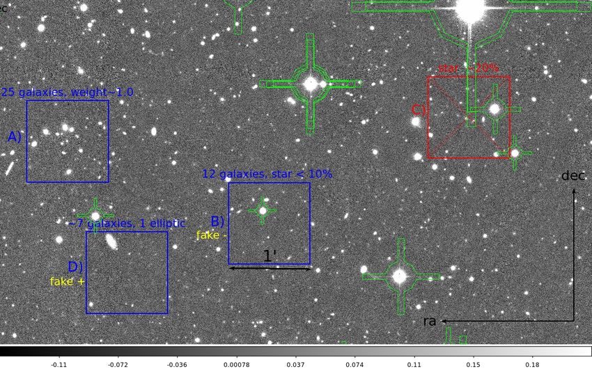
17Figure 3.4: 2D maps of the real space cross-correlation amplitude as a function of the
angular shift
A) between ACT filtered κ map and cs82 κ map. B) Auto-correlation map for ACT filtered
κ map
normalized cross-correlations graphs. However, due to the width of the detection kernel as
well as the existence of long range correlations in the CMB anisotropies those maps contain
a high level of noise and need to be filtered to select a range of modes that are not corrupted
by information unrelated to weak lensing (see H).
The auto-correlation map (Figure G.1) for the ACT non-filtered κ map shows clear
harmonics that emphasize the importance of the filtering step to get rid of those unwanted
correlations. Once filtered from those harmonics, the autocorrelation map tends to be wider
but, though we degraded spatial precision, the cross-correlations with cs82 κ map emerge
from the noise. As shown on Figure 3.4, the peak is shifted from the center by 2 to 3 arcmin.
This is due to a shift in astrometry in some of the initial ACT patches that were
recombined into the cs82 template. So as to correct these errors, astrometry will have to be
checked again and harmonized between patches. One major problem is that the patches we
were provided for this analysis were contiguous but not overlapping. In the next attempt,
working with overlapping patches will allow to correct this effect.
3.3 Fourier space cross-correlations: Prospects
Once the maps are optimized, the next step will be to construct the ~l space cross- power
spectrum. Along with theoretical fits, this could help improve constraints on cosmological
parameters.
Nevertheless, before we can expect any reasonable results, some issues need to be tackled,
the most important one being the effect of the very complex mask used for the cs82 κ map.
Masking the ACT map with the same mask induces parasite peaks in the power spectrum,
that are in the same range as peaks we are expecting to see. A deconvolution step is then
needed to clear the spectrum. Due to the complex structure of the mask, this step turns
out to be the hardest one as can be explained with a quick calculation:
Let T be the spatial κ map and W the mask. Then, with standard definitions, we have:
d2~l
Z
Ť (~x) = W (~x).T (~x) Ť (~l) = .W (~l − ~l0 ).T (~l0 ) (3.1)
(2π]2
18Z
2
hŤ~l ∗ Ť~l0 i = δ(~l − ~l0 ).Č~l Č~l = d2~l0 .|W (~l − ~l0 )2 | .Č~l0 (3.2)
As we are working on pixelised maps, the latter integral can be interpreted as a sum,
which leads us to define the mode coupling matrix as: Č~l = M~l.~l0 .C~l0 . Then we expect to be
able to bin the ~l modes in annuli so as to get Čb = Mbb0 .Cb0
This last step, necessary to the deconvolution is not trivial as the mask is multi-scaled
and has not symmetry or invariance property. The matrix seems to be not invertible.
The next step of this study will then be to introduce both theoretical and semi-empirical
correction to optimize the deconvolution procedure.
19Conclusion
Thus, if, a few decades ago, probing the universe searching for dark matter and unravelling
its large scale structure might have appeared as a hopeless scientific challenge, it is now a
field of its own in modern cosmology and, by pushing forward the limits of previous, well
controlled methods as well as exploring new technics, this project gives very promising
prospects for the analysis of astronomical data and the theoretical deductions with enhanced
precision.
Indeed, not only traditional galaxy weak lensing allows us to infer the projected distri-
bution of dark matter from the distortions in the images of the sources it lenses, but, as a
completely different and unique source, CMB lensing offers new possibilities of high resolu-
tion records that might allow us to get rid of most of systematics and help us understand
structure growth and constrain cosmological parameters...notably through cross-correlation
procedures.
Throughout those months, we tried to explore this idea and develop new methods of
analysis. We were able to reconstruct and test with good precision a dark matter distribution
map on an unusually large patch of the sky, using IDL codes to combine small images,
generate templates, logical masks, shear maps and density maps; and a Fortran90 code to
perform a linear convergence reconstruction. If some errors still need to be corrected with
further processing of the data, notably concerning the astrometry, this first map already
shows high accuracy, especially when compared to cluster distribution in the same redshift
range. The neat cross-correlation peak between our map and a cluster map is the best
evidence of this match.
Given these promising results, we were able to cross-correlate efficiently our data in
real space with data from the ACT CMB lensing survey, which leads the way to great new
possibilities for the detection and analysis our universe structure, including with respect to
redshift.
The next steps will include not only improvement of the astrometry but also design of
new mathematical methods, along with semi-empirical fittings, in order to build Fourier
space cross-correlation maps that we will be able to compare with theoretical models.
20Acknowledgements
I would like to thank thoroughly Pr Eric Linder for his constant supervising and interest,
his great advice and his eagerness to make sure this internship allowed me to develop my
knowledge and skills in cosmology and data analysis as much as possible.
I would like to thank as well Dr. Alexie Leauthaud and Dr. Sudeep Das for their
great help all along this internship, their constant availability and their continued scientific
enthusiasm in the course of our research project; and of course I would like to thank Pr.
Ludovic Van Waerbeke and Dr. Eli Rykoff for their contributions to the data processing
and testing that made this project possible.
Eventually, I would like to tell all the staff from the Lawrence Berkeley National
Laboratory how grateful I am for the warm welcome they gave me and for their friendliness
throughout those four months.
21Bibliography
[1] Leon V.E.Koopmans, Roger D.Blandford, Gravitational Lenses. Physics Today, June
2004.
[2] J.-L Starck, S. Pires, A. Réfrégier, Weak lensing mass reconstruction using wavelets.
Astronomy & Astrophysics, January 2006
[3] M. Bartelmann, P. Schneider, Weak gravitational Lensing. Physics Reports (340),
2001
[4] H. Hoekstra, B. Jain, Weak gravitational lensing and its cosmological applications.
arXiv:0805.0139v, astro-ph, May,2nd 2008
[5] N. Kaiser, G. Squires, Mapping the dark matter with weak gravitational lensing. The
Astrophysical Journal, February,20th 1993
[6] A. Lewis, A. Challinor, Weak gravitational lensing of the CMB. arXiv:0601.594v4,
astro-ph, March,9th 2006
[7] S. Das,D. Spergel, Measuring distance ratios with CMB-galaxy lensing cross-correlations.
arXiv:0810.3931v1, astro-ph, October,21st 2008
[8] E.V. Linder,A. Jenkins Cosmic structure growth and dark energy. arXiv:0305.286v2,
astro-ph, August,20th ,2003
[9] J. Geach, McGill University Stripe82 catalog description website.
http://www.physics.mcgill.ca/ jimgeach/stripe82/,
[10] Emmanuel Bertin official website for Sextractor.
http://www.astromatic.net/software/sextractor,
[11] Princeton University ACT project website. http://www.physics.princeton.edu/act/about.html,
[12] Richard Massey, Jason Rhodes, Richard Ellis, Dark matter maps reveal cosmic scaf-
folding. Nature, vol. 445 05497, letters, 18 January 2007
22List of Figures
1.1 example of elliptic fit . . . . . . . . . . . . . . . . . . . . . . . . . . . . . . . 5
2.1 pre-mask: detection and sorting of parasite structures . . . . . . . . . . . . 8
2.2 Shear averaging: map with pixel size and errors a priori . . . . . . . . . . . 9
2.3 patch from S82p convergence (κ) map with Gaussian smoothing: . . . . . . 10
2.4 Description of different modes . . . . . . . . . . . . . . . . . . . . . . . . . . 12
2.5 Reconstructed maps with signal
noise contours (green). . . . . . . . . . . . . . . . 13
2.6 Source detection from κ maps. . . . . . . . . . . . . . . . . . . . . . . . . . 14
3.1 detection of a high richness cluster by both CMB and galaxy weak lensing
maps . . . . . . . . . . . . . . . . . . . . . . . . . . . . . . . . . . . . . . . . 16
3.2 real space cross-correlations maps. 1 arcmin per pixel . . . . . . . . . . . . 17
3.3 normalized correlation amplitude as a function of the radial shift. . . . . . . 17
3.4 2D maps of the real space cross-correlation amplitude as a function of the
angular shift . . . . . . . . . . . . . . . . . . . . . . . . . . . . . . . . . . . 18
A.1 general pipeline of the project . . . . . . . . . . . . . . . . . . . . . . . . . . 25
B.1 Distribution of sources in the cs82 (dashed pink line) and ACT (dashed blue
line) surveys and consecutive kernels of lensing shear function for cs82 (solid
red line) and ACT CMB map (solid blue line) . . . . . . . . . . . . . . . . . 27
C.1 (1) set of 160 masks of 1 square degree each. (2) combined masks repixelized
(a.) to 1 square arcmin pixel.(3) logical mask for a defined masking threshold. 29
D.1 γ1 map from cs 82 catalog for the template S82p. . . . . . . . . . . . . . . . 31
D.2 logical cluster map from S82 catalog . . . . . . . . . . . . . . . . . . . . . . 31
E.1 κ map patch and large scale structure . . . . . . . . . . . . . . . . . . . . . 33
F.1 General layout of the Stripe82 survey. . . . . . . . . . . . . . . . . . . . . . 35
G.1 real space auto-correlations 2D maps. 1 arcmin per pixel . . . . . . . . . . . 37
G.2 correlation amplitude as a function of the radial shift for theoretical 1D models 37
H.1 ACT calibrated κ maps . . . . . . . . . . . . . . . . . . . . . . . . . . . . . 39
23Appendix A
General pipeline.
24Figure A.1: general pipeline of the project
steps and relations between them. programming languages used: IDL, Python, Fortran90
25Appendix B
kernels in weak lensing
26Figure B.1: Distribution of sources in the cs82 (dashed pink line) and ACT (dashed blue
line) surveys and consecutive kernels of lensing shear function for cs82 (solid red line) and
ACT CMB map (solid blue line)
27Appendix C
Mask processing
Pixels with a product (primary mask surf ace) ∗ (local magnitude of def ect) over a
defined threshold are assigned a proportional value. This creates a pixelized mask with a
continuous scale of values which we need to turn into a logical mask with values 0/1.
We chose a threshold so as to get rid of all the major defects including wide spherical
diffraction halos. Yet pixels with a mask % inferior to the average mask % over the entire
map are left unmasked. As the catalogs were masked before any repixelization it leads to a
lack of shear information in these pixels, which is not a problem unless the pixel richness in
galaxies happens to be really poor. This phenomenon is actually really unlikely due to the
depth of the survey: the same solid angle corresponds to a bigger volume for structures at
higher redshift, which then outnumber the defects (Moreover, they have a better weight).
28Figure C.1: (1) set of 160 masks of 1 square degree each. (2) combined masks repixelized
(a.) to 1 square arcmin pixel.(3) logical mask for a defined masking threshold.
29Appendix D
Example of maps built from cs82
catalog data
30Figure D.1: γ1 map from cs 82 catalog for the template S82p.
Figure D.2: logical cluster map from S82 catalog
31Appendix E
cs82 κ map with positions of
known clusters in this area.
32Figure E.1: κ map patch and large scale structure
blue: high richness clusters (r > 10), 3-circled: very high richness r > 30, redshift range
[0.2; 0.6], red: BOSS low redshift (Appendix F
Stripe82 Layout
3435
blue rectangles: pointings, gap: other survey overlapping Stripe82
Figure F.1: General layout of the Stripe82 survey.
DEC DEC
−1
0
1
−1
0
1
0
S82p1p S82m39m S82m36p
S82p1m S82p2p S82m38m S82m35p
S82p2m S82p3p S82m37m S82m34p
−40
S82p3m S82p4p S82m36m S82m33p
S82p4m S82p5p S82m35m S82m32p
S82p5m S82p6p S82m34m S82m31p
S82p6m S82p7p S82m33m S82m30p
S82p7m S82p8p
S82m32m S82m29p
S82p8m S82p9p
S82m31m S82m28p
S82p10p
S82m30m
S82p9m
10
S82p11p
S82m29m S82m27p
S82p10m S82p12p
S82p11m S82p13p S82m28m
S82m27m S82m26p
S82p14p
S82p12m S82m25p
S82p15p S82m26m
−30
S82p13m S82p16p S82m25m
S82p14m S82p17p S82m24p
S82p15m S82p18p
S82p16m S82p19p
S82p17m S82p20p
S82p18m S82p21p
S82p19m S82p22p
20
S82m24m S82m23p
S82p23p
S82m23m S82m22p
S82p24p
S82p20m S82m22m S82m21p
S82p25p
S82p21m
RA
RA
S82p26p
S82p22m S82m21m S82m20p
S82p27p
S82m19p
−20
S82p23m S82p28p S82m20m
S82p24m S82p29p S82m18p
S82m19m
S82p25m S82p30p S82m17p
S82m18m
S82p26m S82p31p S82m16p
S82p27m S82p32p S82m15p
S82m16m
S82p28m S82p33p S82m14p
S82m15m
30
S82p29m S82p34p
S82m14m S82m13p
S82p35p
S82p30m S82m13m S82m12p
S82p36p
S82p31m S82m12m S82m11p
S82p37p
S82p32m S82m11m S82m10p
S82p38p
S82p33m S82m10m S82m9p
S82p39p
S82p34m S82m9m S82m8p
−10
S82p35m S82p40p S82m8m
S82p41p S82m7m S82m7p
S82p36m
S82p42p S82m6m
S82p37m
S82p43p
S82p38m S82m5m
S82m5p
40
S82p39m S82m4m
S82m4p
S82p40m S82p44p S82m3m
S82m3p
S82p41m S82p45p
S82p46p S82m2p
S82p42m S82m2m
S82p47p S82m1p
S82m1m
S82p43m S82p48p
S82m0m
S82m0p
0Appendix G
Real space cross-correlations
36Figure G.1: real space auto-correlations 2D maps. 1 arcmin per pixel
A) for ACT κ map, B) for cs82 κ map
Figure G.2: correlation amplitude as a function of the radial shift for theoretical 1D models
red:simulated auto-correlations, blue:simulated correlations with cluster map
37Appendix H
ACT maps
38Figure H.1: ACT calibrated κ maps
A)unfiltered map: high level of noise, B)filtered map
39You can also read