ADVERSARIAL MIXUP RESYNTHESIZERS
←
→
Page content transcription
If your browser does not render page correctly, please read the page content below
Arxiv preprint

                                          A DVERSARIAL M IXUP R ESYNTHESIZERS
                                           Christopher Beckham1,3 , Sina Honari1,2 , Alex Lamb1,2 , Vikas Verma†,1,6 , Farnoosh Ghadiri1,3 ,
                                           R Devon Hjelm1,2,5 & Christopher Pal1,3,4,‡∗
                                           1
                                             Mila - Québec Artificial Intelligence Institute, Montréal, Canada
                                           2
                                             Université de Montréal, Canada
                                           3
                                             Polytechnique Montréal, Canada
                                           4
                                             Element AI, Montréal, Canada
                                           5
                                             Microsoft Research, Montréal, Canada
                                           6
                                             Aalto University, Finland
                                           firstname.lastname@mila.quebec
arXiv:1903.02709v2 [stat.ML] 4 Apr 2019

                                           †
                                             vikas.verma@aalto.fi, ‡ christopher.pal@polymtl.ca

                                                                                        A BSTRACT
                                                      In this paper, we explore new approaches to combining information encoded
                                                      within the learned representations of autoencoders. We explore models that are
                                                      capable of combining the attributes of multiple inputs such that a resynthesised
                                                      output is trained to fool an adversarial discriminator for real versus synthesised
                                                      data. Furthermore, we explore the use of such an architecture in the context of
                                                      semi-supervised learning, where we learn a mixing function whose objective is to
                                                      produce interpolations of hidden states, or masked combinations of latent repre-
                                                      sentations that are consistent with a conditioned class label. We show quantitative
                                                      and qualitative evidence that such a formulation is an interesting avenue of re-
                                                      search.

                                          1       I NTRODUCTION
                                          The autoencoder is a fundamental building block in unsupervised learning. Autoencoders are trained
                                          to reconstruct their inputs after being processed by two neural networks: an encoder which encodes
                                          the input to a high-level representation or bottleneck, and a decoder which performs the reconstruc-
                                          tion using the representation as input. One primary goal of the autoencoder is to learn representations
                                          of the input data which are useful (Bengio, 2012), which may help in downstream tasks such as clas-
                                          sification (Zhang et al., 2017; Hsu et al., 2019) or reinforcement learning (van den Oord et al., 2017;
                                          Ha & Schmidhuber, 2018). The representations of autoencoders can be encouraged to contain more
                                          ‘useful’ information by restricting the size of the bottleneck, through the use of input noise (e.g., in
                                          denoising autoencoders, Vincent et al., 2008), through regularisation of the encoder function (Rifai
                                          et al., 2011), or by introducing a prior (Kingma & Welling, 2013). Another goal is in learning in-
                                          terpretable representations (Chen et al., 2016; Jang et al., 2016). In unsupervised learning, learning
                                          often involves qualitative objectives on the representation itself, such as disentanglement of latent
                                          variables (Liu et al., 2017; Thomas et al., 2017) or maximisation of mutual information (Chen et al.,
                                          2016; Belghazi et al., 2018; Hjelm et al., 2019).
                                          Mixup (Zhang et al., 2018) and manifold mixup (Verma et al., 2018) are regularisation techniques
                                          that encourage deep neural networks to behave linearly between two data samples. These methods
                                          artificially augment the training set by producing random convex combinations between pairs of ex-
                                          amples and their corresponding labels and training the network on these combinations. This has the
                                          effect of creating smoother decision boundaries, which can have a positive effect on generalisation
                                          performance. In Verma et al. (2018), the random convex combinations are computed in the hidden
                                          space of the network. This procedure can be viewed as using the high-level representation of the
                                          network to produce novel training examples and provides improvements over strong baselines in the
                                          supervised learning. Furthermore, Verma et al. (2019) propose a simple and efficient method for
                                          semi-supervised classification based on random convex combinations between unlabeled samples
                                          and their predicted labels.
                                              ∗
                                                  Canada CIFAR AI Chair

                                                                                              1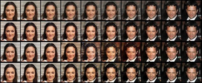
Arxiv preprint

In this paper we explore the use of a wider class of mixing functions for unsupervised learning, mix-
ing in the bottleneck layer of an autoencoder. These mixing functions could consist of continuous
interpolations between latent vectors such as in Verma et al. (2018), to binary masking operations
to even a deep neural network which learns the mixing operation. In order to ensure that the output
of the decoder given the mixed representation resembles the data distribution at the pixel level, we
leverage adversarial learning (Goodfellow et al., 2014), where here we train a discriminator to dis-
tinguish between decoded mixed and unmixed representations. This technique affords a model the
ability to simulate novel data points (such as those corresponding to combinations of annotations not
present in the training set). Furthermore, we explore our approach in the context of semi-supervised
learning, where we learn a mixing function whose objective is to produce interpolations of hidden
states consistent with a conditioned class label.

1.1   R ELATED WORK

Our method can be thought of as an extension of autoencoders that allows for sampling through
mixing operations, such as continuous interpolations and masking operations. Variational autoen-
coders (VAEs, Kingma & Welling, 2013) can also be thought of as a similar extension of autoen-
coders, using the outputs of the encoder as parameters for an approximate posterior q(z|x) which
is matched to a prior distribution p(z) through the evidence lower bound objective (ELBO). At test
time, new data points are sampled by passing samples from the prior, z ∼ p(z), through the de-
coder. In contrast, our we sample a random mixup operation between the representations of two
inputs from the encoder.
The Adversarially Constrained Autoencoder Interpolation (ACAI) method is another approach
which involves sampling interpolations as part of an unsupervised objective (Berthelot* et al., 2019).
ACAI uses a discriminator network to predict the mixing coefficient from the decoder output of
the mixed representation, and the autoencoder tries to ‘fool’ the discriminator, making interpolated
points indistinguishable from real ones. The GAIA algorithm (Sainburg et al., 2018) uses a BEGAN
framework with an additional interpolation-based adversarial objective. What primarily differenti-
ates our work from theirs is that we perform an exploration into different kinds of mixing functions,
including a semi-supervised variant which uses an MLP to produce mixes consistent with a class
label.

2     F ORMULATION
Let us consider an autoencoder model F (·), with the encoder part denoted as f (·) and the decoder
g(·). In an autoencoder we wish to minimise the reconstruction, which is simply:
                                   min Ex∼p(x) ||x − g(f (x))||2                                   (1)
                                     F

Because autoencoders trained by input-reconstruction loss tend to produce images which are slightly
blurry, one can train an adversarial autoencoder (Makhzani et al., 2016), but instead of putting the
adversary on the bottleneck, we put it on the reconstruction, and the discriminator (denoted D) tries
to distinguish between real and reconstructed x, and the autoencoder (which is analogous to the
generator) tries to construct ‘realistic’ reconstructions so as to fool the discriminator. Because of
this, we coin the term ‘ARAE’ (adversarial reconstruction autoencoder). This can be written as:
                        min Ex∼p(x) λ||x − g(f (x))||2 + `GAN (g(f (x)), 1)
                           F
                                                                                                   (2)
                     min Ex∼p(x) `GAN (D(x), 1) + `GAN (D(g(f (x))), 0),
                       D

where `GAN is a GAN-specific loss function. In our case, `GAN is the binary cross-entropy loss,
which corresponds to the Jenson-Shannon GAN (Goodfellow et al., 2014).
One way to use the autoencoder to generate novel samples would be to encode two inputs h1 =
f (x1 ) and h2 = f (x2 ) into their latent representation, perform some combination between them,
and then run the result through the decoder g(·). There are many ways one could combine the two
latent representations, and we denote this function Mix(h1 , h2 ). Manifold mixup (Verma et al.,
2018) implements mixing in the hidden space through convex combinations:
                               Mixmixup (h1 , h2 ) = αh1 + (1 − α)h2 ,                             (3)

                                                  2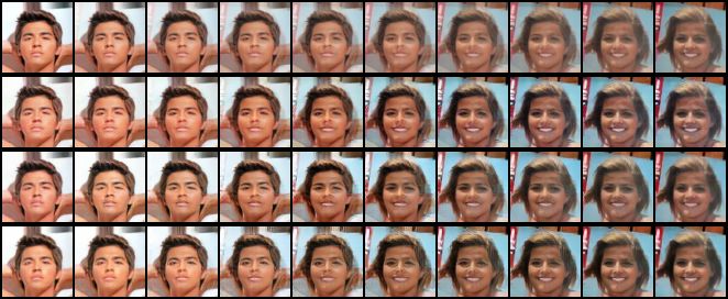
Arxiv preprint

where λ ∈ [0, 1](bs,) is sampled from a Uniform(0, 1) distribution and bs denotes the minibatch size.
In contrast, here we explore a strategy in which we randomly retain some components of the hidden
representation from h1 and use the rest from h2 , and in this case we would randomly sample a binary
mask m ∈ {0, 1}(bs×f ) (where f denotes the number of feature maps) and perform the following
operation:

                               MixBernoulli (h1 , h2 ) = mh1 + (1 − m)h2 ,                               (4)

where m is sampled from a Bernoulli(p) distribution (p can simply be sampled uniformly).
With this in mind, we propose the adversarial mixup resynthesiser (AMR), where part of the au-
toencoder’s objective is to produce mixes which, when decoded, are indistinguishable from real
images. The generator and the discriminator of AMR are trained by the following mixture of loss
components:

   min Ex,x0 ∼p(x) λ||x − g(f (x))||2 + `GAN (g(f (x)), 1) + `GAN (g(Mix(f (x), f (x0 )))), 1) +
    F              |      {z        } |        {z        } |              {z                 }
                         reconstruction    fool D with reconstruction             fool D with mixes
                                                   β||Mix(f (x), f (x )) − f (g(Mix(f (x), f (x0 ))))||2
                                                                         0
                                                   |                       {z                          }
                                                                         mixing consistency

  min Ex,x0 ∼p(x) `GAN (D(x), 1) + `GAN (D(g(f (x))), 0) + `GAN (g(Mix(f (x), f (x0 )))), 0) .
   D              |     {z     } |         {z          } |              {z                 }
                       label x as real    label reconstruction as fake             label mixes as fake
                                                                                                         (5)

Note that the mixing consistency loss is simply the reconstruction between the mix h̃mix =
Mix(f (x), f (x0 )) and the re-encoding of it f (g(h̃mix )), where x and x0 are two randomly sampled
images from the training set. This may be necessary as without it the decoder may simply output an
image which is not semantically consistent with the two images which were mixed (refer to Section
5.2 for an in-depth explanation and analysis of this loss). Both the generator and discriminator are
trained by the decoded image of the mix g(Mix(f (x), f (x0 ))). The discriminator D is trained to
label it as a fake image by minimising its probability and the generator F is trained to fool the dis-
criminator by maximising its probability. Note that the coefficient λ controls the reconstruction and
the coefficient β controls the mixing consistency in the generator. See Figure 1 for a visualisation of
the AMR model.

2.1   U SING LABELS

While it is interesting to generate new examples via random mixing strategies in the hidden states,
we also explore a supervised mixing formulation in which we learn a mixing function that can
produce mixes between two examples such that they are consistent with a particular class label. We
make this possible by backpropagating through a classifier network p(y|x) which branches off the
end of the discriminator, i.e., an auxiliary classifier GAN (Odena et al., 2017).
Let us assume that for some image x, we have a set of binary attributes y associated with it, where
y ∈ {0, 1}k (and k ≥ 1). We introduce a mixing function Mixsup (h1 , h2 , y), which is an MLP that
maps y to Bernoulli parameters p ∈ [0, 1]bs×f . These parameters are used to sample a Bernoulli
mask m ∼ Bernoulli(p) to produce a new combination h̃mix = mh1 + (1 − m)h2 , which is
consistent with the class label y. Note that the conditioning class label should be semantically
meaningful with respect to both of the conditioned hidden states. For example, if we’re producing
mixes based on the gender attribute and both h1 and h2 are male, it would not make sense to
condition on the ‘female’ label. To enforce this constraint, we simply make the conditioning label a
convex combination ỹmix = αy1 + (1 − α)y2 as well, using α ∼ Uniform(0, 1).

                                                       3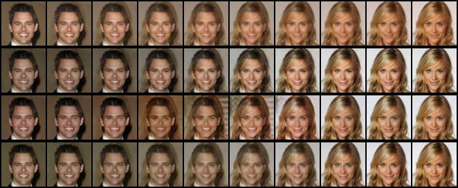
Arxiv preprint

Figure 1: The unsupervised version of the adversarial mixup resynthesiser (AMR). In addition to
the autoencoder loss functions, we have a mixing function Mix which creates some combination
between the latent variables h1 and h2 , which is subsequently decoded into an image intended to
be realistic-looking and semantically consistent with the two constituent images. This is achieved
through the consistency loss (weighted by β) and the discriminator.

To make this more concrete, the autoencoder and discriminator, in addition to their losses described
in Equation 5, try to minimise the following losses:

    min Ex1 ,y2 ∼p(x,y),x2 ,y2 ∼p(x,y),α∼U (0,1) `GAN (D(g(h̃mix )), 1) + `cls (p(y|g(h̃mix )), ỹmix )
     F                                           |       {z           } |             {z             }
                                                          fool D with mix        make mix’s class consistent

                                                                            + β||h̃mix − f (g(h̃mix ))||2
                                                                              |          {z             }
                                                                                      consistency loss         (6)
                                     min Ex1 ,y2 ∼p(x,y),x2 ,y2 ∼p(x,y),α∼U (0,1) `GAN (D(g(h̃mix )), 0)
                                      D                                           |       {z           }
                                                                                       label mixes as fake

                         where ỹmix = αy1 + (1 − α)y2 and h̃mix = Mixsup (f (x1 ), f (x2 ), ỹmix )

Note that for the consistency loss the same coefficient β is used.See Figure 2 for a visualisation of
the supervised AMR model.

3       R ESULTS
We use ResNets (He et al., 2016) for both the generator and discriminator. The precise architectures
for generator and discriminator can be found here.1 The datasets evaluated on are:

          • UT Zappos50K (Yu & Grauman, 2014; 2017): a large dataset comprising 50k images of
            shoes, sandals, slippers, and boots. Each shoe is centered on a white background and in the
            same orientation, which makes it convenient for generative modelling purposes.
          • CelebA (Liu et al., 2015): a large-scale and highly diverse face dataset consisting of 200K
            images. We use the aligned and cropped version of the dataset downscaled to 64px, and
            only consider (via the use of a keypoint-based heuristic) frontal faces. It is worth noting
            that despite this, there is still quite a bit of variation in terms of the size and position of the
            faces, which can make mixing between faces a more difficult task since the faces are not
            completely aligned.

    1
        Link to the code will be added!

                                                        4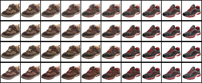
Arxiv preprint

                                                    mixing without labels

                                                       mixing with labels

Figure 2: The supervised version of the adversarial mixup resynthesiser (AMR). The mixer function,
denoted in this figure as Mixsup , takes h1 , h2 and a convex combination of y1 and y2 (denoted ỹmix )
and internally produces a Bernoulli mask which is then used to produce an output combination
h̃mix = mh1 + (1 − m)h2 . h̃mix is then passed to the generator to generate x̃mix . In addition to
fooling the discriminator using x̃mix , the generator also has to make sure the class prediction by the
auxiliary classifier is consistent with the mixed class ỹmix . Note that in this formulation, we still
perform the kind of mixing which was shown in Figure 1, and this is shown in the diagram with the
component noted ‘mixing without labels’.

 PIXEL

 ARAE

 ACAI

 AMR

Figure 3: Interpolations between sheepskin boots and croc shoes for the Zappos dataset. For each
image, from top to bottom, the rows denote: (a) linearly interpolating in pixel space; (b) the ad-
versarial reconstruction autoencoder (ARAE); (c) adversarialy contrained autoencoder interpolation
(ACAI) (Berthelot* et al., 2019) and (d) the adversarial mixup resynthesiser (AMR). For more im-
ages, consult the appendix section.

As seen in Figures 3 and 4, all of the mixup variants produce more realistic-looking interpolations
than in pixel space. Due to background details in CelebA however, it is slightly harder to distin-
guish the quality between the different methods. Though this may not be the most ideal metric to
use in our case (see discussion at end of this section) we use the Frechet Inception Distance (FID)
by Heusel et al. (2017), which is based on features extracted from a pre-trained CelebA classifier,
to compute the distance between samples from the dataset and ones from our autoencoders2 . Con-
cretely, we compute (on the validation set) two scores: the FID between validation samples and their
   2
     This is somewhat of a misnomer because the FID implies the use of an Inception network that has been
pre-trained on ImageNet. Instead, we use a ResNet which has been trained on CelebA.

                                                   5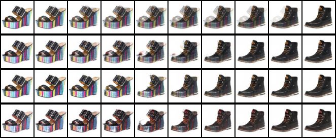
Arxiv preprint
PIXEL
ARAE
ACAI
AMR
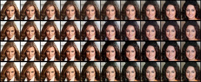
Figure 4: Interpolations between two images for the CelebA dataset, using the mixup technique
(Equation 3). The left-most image is x1 and the right-most image is x2 , and we create mixes between
them by linearly increasing α from 0 to 1. For each image, from top to bottom, the rows denote:
(a) linearly interpolating in pixel space; (b) the adversarial reconstruction autoencoder (ARAE); (c)
adversarially constrained autoencoder interpolation (ACAI) (Berthelot* et al., 2019); and (d) the
adversarial mixup resynthesiser (AMR). For more images, consult the appendix section.
ARAE
AMR
Figure 5: Interpolations between two images for the CelebA dataset, using the Bernoulli mixup
technique (Equation 4). m is sampled from a Bernoulli(p), with zero denoting retain feature maps
from x1 and one denoting retain feature maps from x2 . (Top: ARAE, bottom: AMR)
reconstructions (denoted in the table as FID(data, reconstruction)), and the FID between validation
samples and randomly sampled interpolations (denoted in the table as FID(data, mix)). In the latter
case, we repeat this five times (over five different sets of randomly sampled interpolations) for three
different random seeds, resulting in 5 × 3 = 15 FID scores from which we compute the mean and
standard deviation. These results are shown in Tables 1 and 2 for the mixup and Bernoulli mixup
formulations, respectively.
Table 1: Frechet Inception Distances computed between samples from the validation set and adver-
sarial mixup resynthesiser (AMR) for the mixup loss (Equation 3) in the unsupervised setting. λ and
β denote respectively the reconstruction and consistency coefficients.
Method λ β FID(data, mix) FID(data, reconstruction)
ARAE 20 - 5.94 ± 0.30 1.39 ± 0.13
100 - 4.63 ± 0.22 0.92 ± 0.02
ACAI
50 - 5.10 ± 0.52 1.32 ± 0.46
100 50 4.75 ± 0.26 1.37 ± 0.11
50 50 5.64 ± 0.20 2.59 ± 0.09
AMR (ours)
50 1 4.62 ± 0.20 1.22 ± 0.06
50 0 4.97 ± 0.31 1.26 ± 0.12
6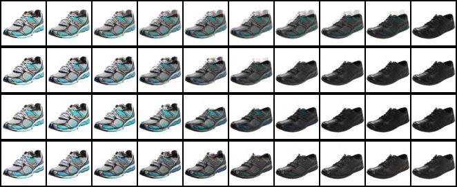
Arxiv preprint

Table 2: Frechet Inception Distances computed between samples from the validation set and adver-
sarial mixup resynthesiser (AMR) for the Bernoulli mixup (Equation 4) technique in the unsuper-
vised setting. λ and β denote respectively the reconstruction and consistency coefficients.

                 Method            λ           β   FID(data, mix)            FID(data, reconstruction)
                 ARAE              20       -         16.64 ± 0.59                             1.39 ± 0.13
                 AMR (ours)        50      50         10.36 ± 0.84                             3.73 ± 0.61

Lower FID is usually considered to be better. However, FID may not be the most appropriate metric
to use in our case. Because the FID is a measure of distance between two distributions, one can
simply obtain a very low FID by simplying autoencoding the data, as shown in Tables 1 and 2. In
the case of mixing, one situation which may favour a lower FID is if g(αf (x1 ) + (1 − α)f (x2 )) ≈
g(f (x1 )) or g(f (x2 )); in other words, the supposed mix simply decodes into one of the original
examples x1 or x2 , which clearly lie on the data manifold. To avoid having the mixed features
αx1 + (1 − α)x2 being decoded back into samples which lie on the data manifold, we leverage
the consistency loss, which is tuned by coefficient β. The lower the coefficient, the more likely that
decoded mixes are projected back onto the manifold, but if this constraint is too weak then it may
not necessarily be desirable if one wants to create novel data points. (For more details, see Section
5.2 in the appendix.)
Despite potential shortcomings of using FID, it seems reasonable to use such a metric to compare
against baselines without any mixing losses, such as the adversarial reconstruction autoencoder
(ARAE), which we indeed outperform for both mixup and Bernoulli mixup. For Bernoulli mixup,
the FID scores appear to be higher than those in the mixup case (Table 1) because the sampled
Bernoulli mask m is also across the channel axis, i.e., it is of the shape (bs, f ), whereas in mixup
α has the shape (bs, ). Because the mixing is performed on an extra axis, this produces a greater
degree of variability in the mixes, and we have observed similar FID scores to the Bernoulli mixup
case by evaluating on a variant of mixup where the α has the shape (bs, f ) instead of (bs, ).

3.1   S UPERVISED C ELEBA

We present some qualitative results with the supervised formulation. We train our supervised AMR
variant using a subset of the attributes in CelebA (‘is male’, ‘is wearing heavy makeup’, and ‘is
wearing lipstick’). We consider pairs of examples {(x1 , y1 ), (x2 , y2 )} (where one example is male
and the other female) and produce random convex combinations of the attributes ỹmix = αy1 + (1 −
α)y2 and decode their resulting mixes Mixsup (f (x1 ), f (x2 ), ỹmix ). This can be seen in Figure 6.

             male       male        male           male           male       male       male        male
             makeup     makeup      makeup         makeup         makeup     makeup     makeup      makeup
             lipstick   lipstick    lipstick       lipstick       lipstick   lipstick   lipstick    lipstick

Figure 6: Interpolations produced by the class mixer function for the set of binary attributes {male,
heavy makeup, lipstick}. For each image, the left-most face is x1 and the right-most face x2 , with
faces in between consisting of mixes Mixsup (f (x1 ), f (x2 ), ỹmix ) of a particular attribute mix ỹmix ,
shown below each column (where red denotes ‘off’ and green denotes ‘on’).

                                                              7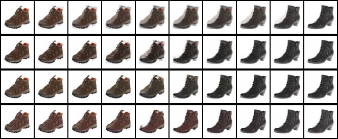
Arxiv preprint

We can see that for the most part, the class mixer function has been able to produce decent mixes
between the two faces consistent with the desired attributes. There are some issues – namely, the
model does not seem to disentangle the lipstick and makeup attributes well – but this may be due
to the strong correlation between lipstick and makeup (lipstick is makeup!), or be in part due to the
classification performance of the auxiliary classifier part of the discriminator (while its accuracy on
both training and validation was as high as 95%, there may still be room for improvement). We
also achieved better results by simply having the embedding function produce a mask m ∈ [0, 1]
rather than {0, 1}, most likely because such a formulation allows a greater degree of flexibility
when it comes to mixing. Indeed, one priority is to conduct further hyperparameter tuning in order
to improve these results. For a visualisation of the Bernoulli parameters output by the embedding
function, see Section 5.4 in the appendix.

4   C ONCLUSION
In this paper, we proposed the adversarial mixup resynthesiser and showed that it can be used
to produce realistic-looking combinations of examples by performing mixing in the bottleneck of
an autoencoder. We proposed several mixing functions, including one based on sampling from
a uniform distribution and the other a Bernoulli distribution. Furthermore, we presented a semi-
supervised version of the Bernoulli variant in which one can leverage class labels to learn a mixing
function which can determine what parts of the latent code should be mixed to produce an image
consistent with a desired class label. While our technique can be used to leverage an autoencoder
as a generative model, we conjecture that our technique may have positive effects on the latent
representation and therefore downstream tasks, though this is yet to be substantiated. Future work
will involve more comparisons to existing literature and experiments to determine the effects of
mixing on the latent space itself and downstream tasks.

ACKNOWLEDGMENTS
We thank Huawei for supporting this research. We also thank Compute Canada for GPUs used in
this work. Vikas Verma was supported by Academy of Finland project 13312683 / Raiko Tapani AT
kulut.

R EFERENCES
Mohamed Ishmael Belghazi, Aristide Baratin, Sai Rajeshwar, Sherjil Ozair, Yoshua Bengio, Aaron
 Courville, and Devon Hjelm. Mutual information neural estimation. In Jennifer Dy and Andreas
 Krause (eds.), Proceedings of the 35th International Conference on Machine Learning, volume 80
 of Proceedings of Machine Learning Research, pp. 531–540, Stockholmsmssan, Stockholm Swe-
 den, 10–15 Jul 2018. PMLR.
Yoshua Bengio. Deep learning of representations for unsupervised and transfer learning. In Isabelle
  Guyon, Gideon Dror, Vincent Lemaire, Graham Taylor, and Daniel Silver (eds.), Proceedings of
  ICML Workshop on Unsupervised and Transfer Learning, volume 27 of Proceedings of Machine
  Learning Research, pp. 17–36, Bellevue, Washington, USA, 02 Jul 2012. PMLR.
David Berthelot*, Colin Raffel*, Aurko Roy, and Ian Goodfellow. Understanding and improv-
  ing interpolation in autoencoders via an adversarial regularizer. In International Conference on
  Learning Representations, 2019.
Xi Chen, Yan Duan, Rein Houthooft, John Schulman, Ilya Sutskever, and Pieter Abbeel. Infogan:
  Interpretable representation learning by information maximizing generative adversarial nets. In
  Advances in neural information processing systems, pp. 2172–2180, 2016.
Ian Goodfellow, Jean Pouget-Abadie, Mehdi Mirza, Bing Xu, David Warde-Farley, Sherjil Ozair,
  Aaron Courville, and Yoshua Bengio. Generative adversarial nets. In Advances in neural infor-
  mation processing systems, pp. 2672–2680, 2014.
David Ha and Jürgen Schmidhuber. Recurrent world models facilitate policy evolution. In Advances
  in Neural Information Processing Systems 31, pp. 2451–2463. Curran Associates, Inc., 2018.
  https://worldmodels.github.io.

                                                  8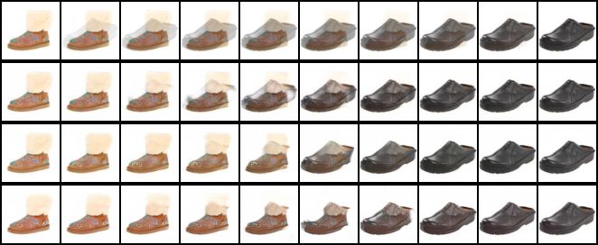
Arxiv preprint

Kaiming He, Xiangyu Zhang, Shaoqing Ren, and Jian Sun. Deep residual learning for image recog-
  nition. In Proceedings of the IEEE conference on computer vision and pattern recognition, pp.
  770–778, 2016.

Martin Heusel, Hubert Ramsauer, Thomas Unterthiner, Bernhard Nessler, and Sepp Hochreiter.
 Gans trained by a two time-scale update rule converge to a local nash equilibrium. In Advances
 in Neural Information Processing Systems, pp. 6626–6637, 2017.

R Devon Hjelm, Alex Fedorov, Samuel Lavoie-Marchildon, Karan Grewal, Phil Bachman, Adam
  Trischler, and Yoshua Bengio. Learning deep representations by mutual information estimation
  and maximization. In International Conference on Learning Representations, 2019.

Kyle Hsu, Sergey Levine, and Chelsea Finn. Unsupervised learning via meta-learning. In Interna-
  tional Conference on Learning Representations, 2019.

Eric Jang, Shixiang Gu, and Ben Poole. Categorical reparameterization with gumbel-softmax. arXiv
  preprint arXiv:1611.01144, 2016.

Diederik P Kingma and Max Welling.           Auto-encoding variational bayes.      arXiv preprint
  arXiv:1312.6114, 2013.

Ming-Yu Liu, Thomas Breuel, and Jan Kautz. Unsupervised image-to-image translation networks.
 In I. Guyon, U. V. Luxburg, S. Bengio, H. Wallach, R. Fergus, S. Vishwanathan, and R. Garnett
 (eds.), Advances in Neural Information Processing Systems 30, pp. 700–708. Curran Associates,
 Inc., 2017.

Ziwei Liu, Ping Luo, Xiaogang Wang, and Xiaoou Tang. Deep learning face attributes in the wild.
  In Proceedings of International Conference on Computer Vision (ICCV), 2015.

Alireza Makhzani, Jonathon Shlens, Navdeep Jaitly, and Ian Goodfellow. Adversarial autoencoders.
  In International Conference on Learning Representations, 2016.

Takeru Miyato, Toshiki Kataoka, Masanori Koyama, and Yuichi Yoshida. Spectral normalization
  for generative adversarial networks. In International Conference on Learning Representations,
  2018.

Augustus Odena, Christopher Olah, and Jonathon Shlens. Conditional image synthesis with auxil-
  iary classifier gans. In Proceedings of the 34th International Conference on Machine Learning-
  Volume 70, pp. 2642–2651. JMLR. org, 2017.

Salah Rifai, Pascal Vincent, Xavier Muller, Xavier Glorot, and Yoshua Bengio. Contractive auto-
  encoders: Explicit invariance during feature extraction. In Proceedings of the 28th International
  Conference on International Conference on Machine Learning, ICML’11, pp. 833–840, USA,
  2011. Omnipress. ISBN 978-1-4503-0619-5.

Tim Sainburg, Marvin Thielk, Brad Theilman, Benjamin Migliori, and Timothy Gentner. Gener-
  ative adversarial interpolative autoencoding: adversarial training on latent space interpolations
  encourage convex latent distributions. CoRR, abs/1807.06650, 2018.

Valentin Thomas, Jules Pondard, Emmanuel Bengio, Marc Sarfati, Philippe Beaudoin, Marie-Jean
  Meurs, Joelle Pineau, Doina Precup, and Yoshua Bengio. Independently controllable factors.
  CoRR, abs/1708.01289, 2017.

Aaron van den Oord, Oriol Vinyals, and koray kavukcuoglu. Neural discrete representation learning.
  In I. Guyon, U. V. Luxburg, S. Bengio, H. Wallach, R. Fergus, S. Vishwanathan, and R. Garnett
  (eds.), Advances in Neural Information Processing Systems 30, pp. 6306–6315. Curran Asso-
  ciates, Inc., 2017.

Vikas Verma, Alex Lamb, Christopher Beckham, Aaron Courville, Ioannis Mitliagkis, and Yoshua
  Bengio. Manifold mixup: Encouraging meaningful on-manifold interpolation as a regularizer.
  arXiv preprint arXiv:1806.05236, 2018.

                                                9
Arxiv preprint
Vikas Verma, Alex Lamb, Juho Kannala, Yoshua Bengio, and David Lopez-Paz. Interpolation
Consistency Training for Semi-Supervised Learning. arXiv e-prints, art. arXiv:1903.03825, Mar
2019.
Pascal Vincent, Hugo Larochelle, Yoshua Bengio, and Pierre-Antoine Manzagol. Extracting and
composing robust features with denoising autoencoders. In Proceedings of the 25th International
Conference on Machine Learning, ICML ’08, pp. 1096–1103, New York, NY, USA, 2008. ACM.
ISBN 978-1-60558-205-4. doi: 10.1145/1390156.1390294.
A. Yu and K. Grauman. Fine-grained visual comparisons with local learning. In Computer Vision
and Pattern Recognition (CVPR), Jun 2014.
A. Yu and K. Grauman. Semantic jitter: Dense supervision for visual comparisons via synthetic
images. In International Conference on Computer Vision (ICCV), Oct 2017.
Hongyi Zhang, Moustapha Cisse, Yann N. Dauphin, and David Lopez-Paz. mixup: Beyond empiri-
cal risk minimization. International Conference on Learning Representations, 2018.
Richard Zhang, Phillip Isola, and Alexei A Efros. Split-brain autoencoders: Unsupervised learning
by cross-channel prediction. In Proceedings of the IEEE Conference on Computer Vision and
Pattern Recognition, pp. 1058–1067, 2017.
10Arxiv preprint
5 A PPENDIX
5.1 E XPERIMENTAL CONFIGURATION
We will provide a summary of our experimental setup here, though we also provide links to (and
encourage viewers to look at) various parts of the code such as the networks used for the generator
and discriminator and the optimiser hyperparameters.
We use a residual network for both the generator and discriminator. The discriminator uses spec-
tral normalisation (Miyato et al., 2018), with five discriminator updates being performed for each
generator update. We use ADAM for our optimiser with α = 2e−4 , β1 = 0.0 and β2 = 0.99.
11Arxiv preprint
5.2 C ONSISTENCY LOSS
In order to examine the effect of the consistency loss, we explore a simple two-dimensional spiral
dataset, where points along the spiral are deemed to be part of the data distribution and points outside
it are not. With the mixup loss enabled and λ = 10, we try values of β ∈ {0, 0.1, 10, 100}. After
100 epochs of training, we produce decoded random mixes and plot them over the data distribution,
which are shown as orange points (overlaid on top of real samples, shown in blue). This is shown in
Figure 7.
As we can see, the lower β is, the more likely interpolated points will lie within the data manifold
(i.e. the spiral). This is because the consistency loss competes with the discriminator loss – as β is
decreased, there is a relatively greater incentive for the autoencoder to try and fool the discriminator
with interpolations, forcing it to decode interpolated points such that they lie in the spiral. Ideally
however we would want a bit of both: we want high consistency so that interpolations in hidden
states are semantically meaningful (and do not decode into some other random data point), while
also having those decoded interpolations look realistic.
Figure 7: Experiments on AMR on the spiral dataset, showing the effect of the consistency loss
β. Decoded interpolations (shown as orange) are overlaid on top of the real data (shown as blue).
Interpolations are defined as ||h̃mix − f (g(h̃mix ))||2 (where h̃mix = αf (x1 ) + (1 − α)f (x2 ) and
α ∼ U (0, 1) for randomly sampled {x1 , x2 })
We also compare our formulation to ACAI (Berthelot* et al., 2019), which does not explicitly have
a consistency loss term. Instead, the discriminator tries to predict what the mixing coefficient α is,
and the autoencoder tries to fool it into thinking interpolations have a coefficient of 0. In Figure
8 we compare this to our formulation in which β = 0. This is shown in Figure 8a (right figure).
It appears that ACAI also prefers to place points in the spiral, although not as strongly as AMR
with β = 0 (though this may be because ACAI needs to trained for longer – ACAI and AMR were
trained for the same number of epochs). In Figure 8b we can see that over the course of training
the consistency losses for both ACAI and AMR gradually rise, indicating both models’ preference
for moving interpolated points closer to the data manifold. Note that here we are only observing the
consistency loss during training, and it is not used in the generator’s loss.
Lastly, in Figure 9 we show some side-by-side comparisons of our model interpolating between
faces when β = 50 and β = 0. We can see that when β = 0 interpolations between faces are not
as smooth in terms of colour and lighting. This somewhat slight discontinuity in the interpolation
12Arxiv preprint
may be explained by the decoder pushing these interpolated points closer to the data manifold, since
there is no consistency loss enforced.
(a) Left: AMR with λ = 10, β = 0; right: ACAI with λ = 10 (β = 0 since ACAI does not enforce a
consistency loss). AMR was trained for 200 epochs and ACAI for 300 epochs, since ACAI takes longer to
converge.
0.30
0.20
consistency
0.10
AMR, beta=0
ACAI
0.00
0 50 100 150 200
epoch
(b) Consistency loss plotted for both AMR (black) and ACAI (red).
Figure 8: Comparisons between ACAI (λ = 10) and AMR (λ = 10, β = 0) on the 2D spiral dataset.
Top figure: decoded interpolations (shown as orange) overlaid on top of the real data (shown as blue);
bottom: plot of the consistency loss ||h̃mix − f (g(h̃mix ))||2 (where h̃mix = αf (x1 ) + (1 − α)f (x2 )
and α ∼ U (0, 1) for randomly sampled {x1 , x2 }) over the course of training.
β = 50
β =0
β = 50
β =0
Figure 9: Interpolations using AMR {λ = 50, β = 50} and {λ = 50, β = 0}.
13Arxiv preprint
5.3 L ATENT SPACE VISUALISATION
For both the adversarial reconstruction autoencoder (ARAE) and our adversarial mixup resynthe-
siser (AMR) we compute a t-SNE on the latent codes produced from the training set of MNIST and
compute the mean of each cluster (where clusters are determined based on running the K-Means
algorithm and setting the number of clusters to be the number of actual classes in the dataset). From
this, we compute pairwise distances between the clusters and compute the mean over this, which is
the average inter-cluster distance. We run the t-SNE algorithm five times for three random seeds,
resulting in 5 × 3 = 15 average inter-cluster distances. We compute the mean and standard deviation
over this. Specifically, we are interested if there are any statistically significant differences between
the average inter-cluster distances between the baseline and our method, as this could be indicative
of topological changes in the latent space influenced by our mixup formulation. We train different
AMR models where β ∈ {200, 100, 50} and λ = 50, and also run an ARAE baseline for λ = 50.
These are shown below in Figure 10.
10_mnist_mixup_g16_frontal_bid_lamb50_beta0_inorm 10_mnist_mixup_g16_frontal_bid_lamb50_beta50_inorm
1 9
4 8
5 3
9 6 2 7 1
3 2
0 5 6
4
7 8 0
4.059006 ± 0.170756 4.343141 ± 0.144256
10_mnist_baseline_g16_frontal_bid_lamb50_inorm
5
8 0
7 2
4 3
9
6 1
4.089527 ± 0.134623
10_mnist_acai_g16_frontal_bid_lamb50_inorm 10_mnist_acai_g16_frontal_bid_lamb50_beta50_inorm
3 7 8
2
7 1
5 4
2 0 1 5 9
9 6
8 0
4 6 3
4.218688 ± 0.174262 4.296465 ± 0.172314
Figure 10: Top-left: AMR with λ = 50, β = 0; top-right: AMR with λ = 50, β = 50; center:
ARAE with λ = 50; bottom-left: ACAI with λ = 50, β = 0; bottom-right: ACAI with λ = 50, β =
50. For each plot, the number shown in orange is the mean inter-cluster distance (averaged over 5
t-SNE seeds and 3 model seeds) and standard deviation. (Note: the numbers associated with each
label denote the cluster centroid, not the MNIST digit.)
14Arxiv preprint
These figures provide evidence that both our method and ACAI may be inducing some topological
changes in latent space. For example, for ACAI (bottom-left with {λ = 50, β = 0}, and bottom-
right with {λ = 50, β = 50}) the average inter-cluster distances are significantly greater than that
of the ARAE baseline shown in the center (though the difference between the two ACAI runs are
not significant, with a paired t-test p-value of 0.1702 > 0.05). Our method on the other hand with
{λ = 50, β = 0} (top-left) is not significantly different from the baseline, but as soon as we add the
consistency loss β = 50 we achieve a much greater (and statistically significant) increase in average
inter-cluster distance. Overall, we can see that both our mixup and ACAI achieves higher average
inter-cluster distances than the baseline, but an exploration into why this is the case is necessary.
Lastly, it is worth noting that Berthelot* et al. (2019) experimented with training linear classifiers
on top of the latent spaces learned by various autoencoders and found their method produced the
highest accuracy. If we assume the clusters represent distinct classes in the dataset and that these are
further apart from each other with a mixup formulation (like what we have seen in Figure 10) then
we would expect a linear classifier to have an easier job placing decision boundaries between them.
If this is the case, then our t-SNE results here corroborate their empirical results.
5.4 B ERNOULLI PARAMETERS FROM SUPERVISED AMR
To recap, the class mixer in the supervised formulation internally maps from a label ỹmix to Bernoulli
parameters p ∈ [0, 1]K , from which a Bernoulli mask m ∼ Bernoulli(p) is sampled. The result-
ing Bernoulli parameters p are shown in Figure 11, where each row denotes some combination of
attributes y ∈ {000, 001, 010, . . . } and the columns denote the index of p (spread out across four
images, such that the first image denotes p1:128 , second image p128:256 , etc.). We can see that each
attribute combination spells out a binary combination of feature maps, which allows one to easily
glean which feature maps contribute to which attributes.
Figure 11: Visualisation of Bernoulli parameters p internally produced by the class mixer function.
Rows denote attribute combinations y and columns denote the index of p.
5.5 A DDITIONAL SAMPLES
In this section we show additional samples of the AMR model (using mixup and Bernoulli mixup
variants) on Zappos and CelebA datasets. We compare AMR against linear interpolation in pixel
space (pixel), adversarial reconstruction autoencoder (ARAE), and adversarialy contrained autoen-
coder interpolation (ACAI). As can be observed in the following images, the interpolations of pixel
and ARAE are less realistic and suffer from more artifacts. AMR and ACAI produce more realistic-
looking results, while AMR generates a smoother transition between the two samples.
• Figure 12: AMR on Zappos (mixup)
• Figure 13: AMR on Zappos (Bernoulli mixup)
• Figure 14: AMR on CelebA (mixup)
• Figure 15: AMR on CelebA (Bernoulli mixup)
• Figure 16: AMR on CelebA-HQ (Bernoulli mixup)
• Figure 17: AMR on Zappos-HQ (Bernoulli mixup)
15Arxiv preprint
PIXEL
ARAE
ACAI
AMR
Figure 12: Interpolations between two images using the mixup technique (Equation 3). For each
image, from top to bottom, the rows denote: (a) linearly interpolating in pixel space; (b) ARAE; (c)
ACAI (Berthelot* et al., 2019); and (d) AMR.
16Arxiv preprint
ARAE
AMR
Figure 13: Interpolations between two images using the Bernoulli mixup technique (Equation 3).
For each image, from top to bottom, the rows denote: (a) ARAE; and (b) AMR.
17Arxiv preprint
PIXEL
ARAE
ACAI
AMR
Figure 14: Interpolations between two images using the mixup technique (Equation 3). For each
image, from top to bottom, the rows denote: (a) linearly interpolating in pixel space; (b) ARAE; (c)
ACAI; and (d) AMR.
18Arxiv preprint
ARAE
AMR
Figure 15: Interpolations between two images using the Bernoulli mixup technique (Equation 4).
(For each image, top: ARAE, bottom: AMR)
19Arxiv preprint
Figure 16: Interpolations between two images using the Bernoulli mixup technique (Equation 4).
Each row is AMR.
20Arxiv preprint
Figure 17: Interpolations between two images using the Bernoulli mixup technique (Equation 4).
Each row is AMR.
21You can also read