Using Geogebra - for Origami - Foldworks
←
→
Page content transcription
If your browser does not render page correctly, please read the page content below
Using Geogebra

     for
   Origami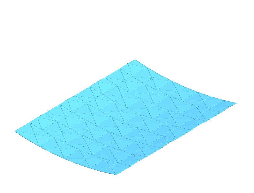
©2021 Tung Ken Lam

Tung Ken Lam asserts his moral right to be identified as the author of this work.
You may use this work for personal and non-commercial educational purposes.
All other rights reserved.

                                              Tung Ken Lam www.foldworks.net

                                       ii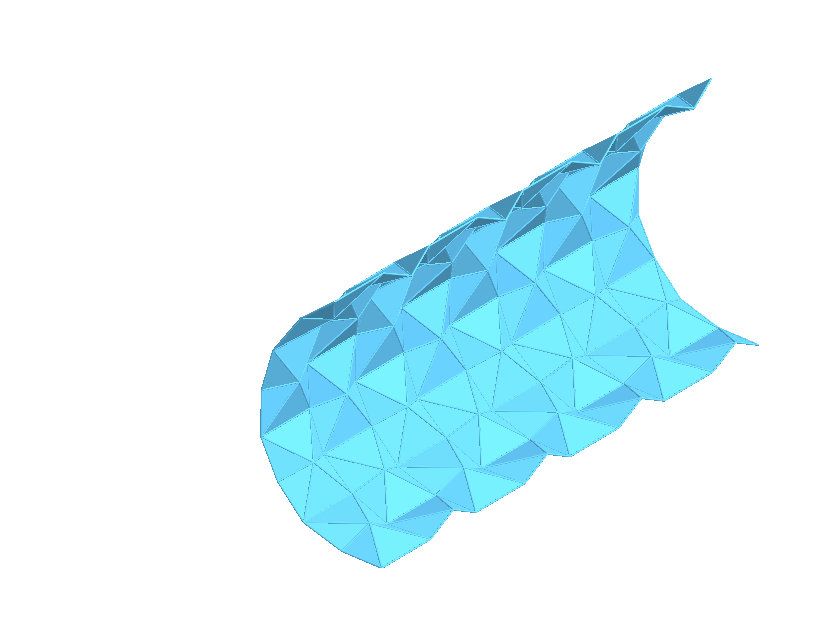
Contents

1 Using Geogebra for Origami                                                                                  1
  1.1 What is Dynamic Geometry Software?          .   .   .   .   .   .   .   .   .   .   .   .   .   .   .   1
  1.2 Why use Geogebra for Origami? . . . .       .   .   .   .   .   .   .   .   .   .   .   .   .   .   .   1
      1.2.1 Design . . . . . . . . . . . . . .    .   .   .   .   .   .   .   .   .   .   .   .   .   .   .   1
      1.2.2 Draw . . . . . . . . . . . . . . .    .   .   .   .   .   .   .   .   .   .   .   .   .   .   .   1
      1.2.3 Animate . . . . . . . . . . . . .     .   .   .   .   .   .   .   .   .   .   .   .   .   .   .   1
  1.3 Learning to use Geogebra for origami .      .   .   .   .   .   .   .   .   .   .   .   .   .   .   .   2
      1.3.1 Beginner . . . . . . . . . . . . .    .   .   .   .   .   .   .   .   .   .   .   .   .   .   .   2
      1.3.2 Intermediate . . . . . . . . . . .    .   .   .   .   .   .   .   .   .   .   .   .   .   .   .   3
      1.3.3 Advanced . . . . . . . . . . . .      .   .   .   .   .   .   .   .   .   .   .   .   .   .   .   4

2 Modelling Origami in Geogebra                                                                               6
  2.1 Two approaches for modelling origami . . . . . . . . . . . . . .                                .   .   6
      2.1.1 Make accurate models . . . . . . . . . . . . . . . . . .                                  .   .   6
      2.1.2 Make models that look right even if inaccurate . . . . .                                  .   .   6
  2.2 General tips for construction . . . . . . . . . . . . . . . . . . .                             .   .   6
      2.2.1 Exploit symmetry . . . . . . . . . . . . . . . . . . . . .                                .   .   6
      2.2.2 Use meaningful variables and conventions . . . . . . .                                    .   .   6
  2.3 Modelling paper . . . . . . . . . . . . . . . . . . . . . . . . . .                             .   .   7
      2.3.1 Use (Z) layer to stack polygons in the correct order .                                    .   .   7
      2.3.2 Avoid self-intersection or simulate double-sided paper                                    .   .   7
  2.4 Making the most of Geogebra . . . . . . . . . . . . . . . . . .                                 .   .   7
      2.4.1 Variable opacity . . . . . . . . . . . . . . . . . . . . . .                              .   .   7
      2.4.2 Some shortcuts . . . . . . . . . . . . . . . . . . . . . .                                .   .   7
      2.4.3 Workspace . . . . . . . . . . . . . . . . . . . . . . . .                                 .   .   7
      2.4.4 2D and 3D . . . . . . . . . . . . . . . . . . . . . . . . .                               .   .   7
      2.4.5 Graphics, Graphics 2 and 3D . . . . . . . . . . . . . .                                   .   .   8
  2.5 Advanced tips . . . . . . . . . . . . . . . . . . . . . . . . . . .                             .   .   8
      2.5.1 Control . . . . . . . . . . . . . . . . . . . . . . . . . .                               .   .   8
      2.5.2 Custom tool . . . . . . . . . . . . . . . . . . . . . . . .                               .   .   8
      2.5.3 Use Sequence[] to make a list object . . . . . . . . .                                    .   .   9

3 Animation                                                                                                   10
  3.1 Use variables and sliders to animate models         .   .   .   .   .   .   .   .   .   .   .   .   .   10
  3.2 Nonlinear animation . . . . . . . . . . . . .       .   .   .   .   .   .   .   .   .   .   .   .   .   12
  3.3 Multistage animation . . . . . . . . . . . . .      .   .   .   .   .   .   .   .   .   .   .   .   .   12
  3.4 Use graphs to animate multiple objects . .          .   .   .   .   .   .   .   .   .   .   .   .   .   13
  3.5 Using the clock to avoid bad key frames . .         .   .   .   .   .   .   .   .   .   .   .   .   .   13

                                       iii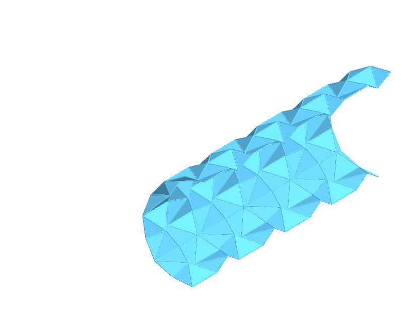
4 Step-by-Step                                                              15
  4.1 The Magic Star: an efficient method . . . . . . . . . . . . . . . . . 15
  4.2 The Magic Star: a GUI-only method . . . . . . . . . . . . . . . . . 25
  4.3 The Four Square Flexagon . . . . . . . . . . . . . . . . . . . . . . 32

                                      iv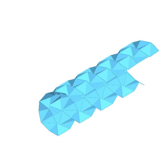
Chapter 1

Using Geogebra for Origami

1.1     What is Dynamic Geometry Software?
If you have not used a Dynamic Geometry Software (DGS) program before, think
of it as flexible vector drawing program. Of course, it can be more powerful
than that. Examples of DGS software include Cabri and Geometer’s Sketchpad.
Geogebra is free to use.

1.2     Why use Geogebra for Origami?
These are some of the tasks that DGS can help with:

1.2.1    Design
   • Test and check geometry: e.g. does that intersection of lines really locate
     the point that you think it does?

   • Generalise a design e.g. change from a square to an oblong, or change from
     a square to a regular pentagon or hexagon.

1.2.2    Draw
   • Virtually fold a flap

   • Vary a design e.g. change the number of units and/or key angle used

   • Export to PDF for editing

   • Construct a 3D model and export it as an image or 3D file

1.2.3    Animate
   • Animate an action model

   • Export to animated GIF

   • Rotate a model in 3D

                                      1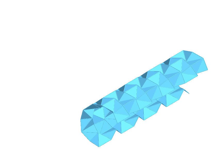
1.3. Learning to use Geogebra for origami

    Files to view and edit are at www.geogebra.org/u/tung+ken+lam.
    A positive side-effect is that your geometric and spatial thinking will improve
as you switch between the physical and digital worlds. Your understanding of
folding will be deeper: paper doesn‘t intersect itself, but simulations will unless
you take corrective steps. You will also learn the limitations of both media.
    These notes were originally written to accompany the animated table of con-
tents for the book Action Modular Origami to Intrigue and Delight.

1.3      Learning to use Geogebra for origami
These are some typical steps in learning from beginner to advanced levels:

1.3.1     Beginner

                        Figure 1.1: Beginner constructions

    • Construct a square in a naive way

    • Robust construction of a square or silver rectangle

    • Virtually fold a flap of paper (reflect points)

    • Use Graphics 2 for a “clean” view for exporting: keep Graphics (1) for
      editing (figure 1.1)

                                          2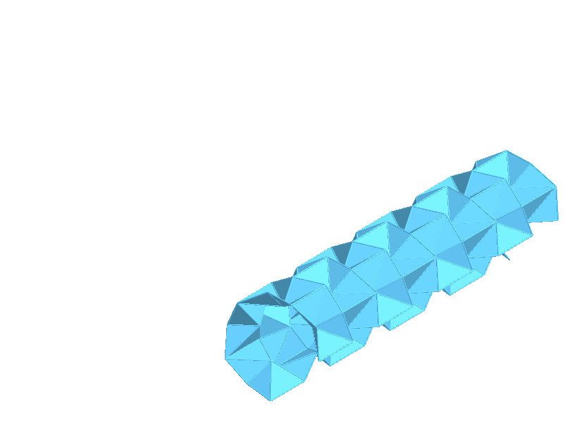
1.3. Learning to use Geogebra for origami

1.3.2     Intermediate

             Figure 1.2: Intermediate construction: fold a flap in 3D

    • Construct a rectangle of proportions 1:n

    • Input Bar for expressions and definitions

    • Use a slider to change the value of a variable editing

    • Animate a construction using a slider for export to an animated GIF

    • 3D constructions e.g. rotate a flap (figure 1.2)

                                        3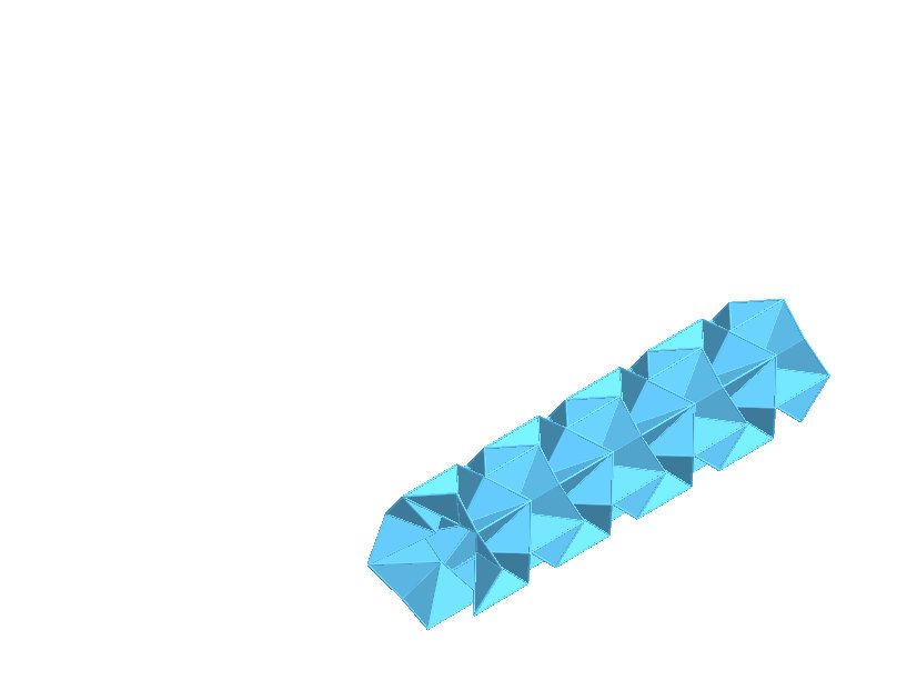
1.3. Learning to use Geogebra for origami
1.3.3 Advanced
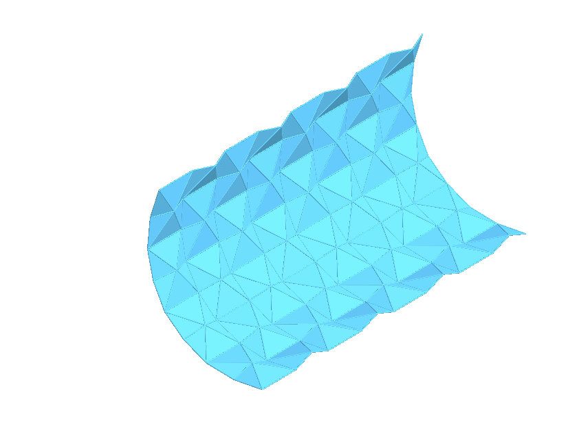
Figure 1.3: Advanced construction: inside reverse fold
Figure 1.4: Advanced construction: inside reverse fold, alternative method
4
1.3. Learning to use Geogebra for origami

                     Figure 1.5: Advanced construction: lists

    • 3D constructions e.g. inside reverse fold in half of a waterbomb base (fig-
      ure 1.3 and figure 1.4)

    • Use lists to amalgamate and process objects e.g. list1 = {a,b,c}

    • Sequence[] command for repeated actions in a loop like For ... Next e.g.
      rotate an object eight times around a centre of rotation (figure 1.5), or
      translate an object in rows and columns to fill the plane, or make n-sided
      polygons of a constant size given a centre and vertex (the built-in polygon
      tool takes two points and the number of sides as arguments, so the more
      sides, the bigger the polygon), etc.

    • Test for definition of objects and conditional formatting e.g. hide/show an
      object

    • Nonlinear animation (slow-in and slow-out)

    • Custom tool

    After this list of ideas and techniques to try, you will find step-by-step exam-
ples of how to make some specific origami models in Geogebra.

                                         5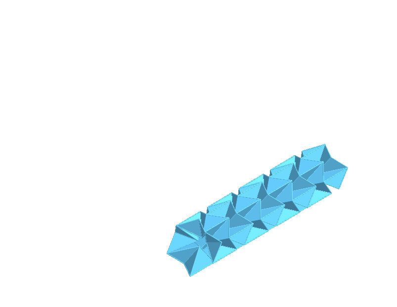
Chapter 2

Modelling Origami in Geogebra

2.1      Two approaches for modelling origami
2.1.1     Make accurate models
Naïve users sometimes create objects by eye instead of constructing them mathe-
matically. For example, check that a 60◦ angle is 60◦ , not 62.7◦ , say, when created
by eye.

2.1.2     Make models that look right even if inaccurate
Sometimes it’s expedient to accept a small error for the right visual effect e.g.
Double Skew Tetrahedra has some faces that change size slightly as they rotate,
even though they should stay the same.

2.2      General tips for construction
2.2.1     Exploit symmetry
Magic Star: spiral version has eight units: four blue and four orange. Instead of
defining eight units by defining eight polygons from eight sets of points, use a
centre of rotation and a rotation angle to define the eight units.

2.2.2     Use meaningful variables and conventions
If you do not specify variable names then they are automatically assigned. This is
usually ok, but non-trivial constructions benefit from meaningful variable names
or conventions e.g. Point O is the centre or origin. You can colour and format
the objects to help organise them e.g. a large red point is meant to be dragged
on screen to change the construction. Avoid using light colours if possible as
associated text is hard to read on a white background.

                                         6
2.3. Modelling paper
2.3 Modelling paper
2.3.1 Use (Z) layer to stack polygons in the correct
order
The paper flaps of Ribbon Slider are modelled as separate polygons. In order for
the layers to be shown in the correct order, set the Layer value between 0 and 9
(9 is the uppermost layer).
2.3.2 Avoid self-intersection or simulate double-sided
paper
The (Z) layer property might not work as you expect for 3D models. Offset
polygons by a small angle or vector so that they render as separate objects.
This technique can be used to simulate paper with different colours on each
side. However, this may need extra work if the polygons rotate e.g. when the
first rotation of Jacob’s Ladder reaches 90◦ , the colours of the two polygons flip
over to simulate double-sided paper.
2.4 Making the most of Geogebra
2.4.1 Variable opacity
Sometimes it’s helpful to have transparent polygons during construction. How-
ever, you want usually opaque objects for the finished model: instead of setting
the opacity of each object, use a slider for opacity and set it into the object’s prop-
erties. This makes it easy to go back to transparent polygons when you want to
change the construction. Note that zero opacity gives wireframe views.
2.4.2 Some shortcuts
Press Ctrl-A for α, Ctrl-B for β, etc and Ctrl-O for ◦ .
2.4.3 Workspace
You can drag the window pane titles to split the window in ways that are helpful
for you e.g. figure 3.4 has the algebra pane above the graphics pane so that long
definitions can be seen without scrolling.
Use Options > Rounding for more or less precision. You can switch between
seeing values and definitions in the algebra pane by pressing Cmd-‘.
2.4.4 2D and 3D
If some 3D commands do not work as expected, check that the inputs are 3D
e.g. change point A(1,2) to A(1,2,0).
72.5. Advanced tips
Figure 2.1: Use a slider to control how to interact with the model
2.4.5 Graphics, Graphics 2 and 3D
Use the Advanced Object Properties to show or hide an object in these views.
For a 2D model you could have a clean view in Graphics 2 but show construction
objects in Graphics.
2.5 Advanced tips
2.5.1 Control
Sometimes you want to control your model in different ways: e.g. in Petrie-Coxeter
Honeycomb you can manually set individual sliders, move the point in the triangle
to set all three angles or animate using the clock variable (Figure 2.1). Each angle
uses nested If[] commands to select the appropriate angle. Note the “set sliders
90°” button uses the simple script shown in the figure.
2.5.2 Custom tool
If you find yourself repeatedly doing the same steps, you could use the Sequence[]
command and/or create a custom tool e.g. Radioactive Ball has custom tool
ProjectPointOnSphere[ , , ].
82.5. Advanced tips
2.5.3 Use Sequence[] to make a list object
Instead of rotating an object three times to make four objects, use the Sequence[]
command to create a list object that rotates the object four times. This saves time
and helps to organise the model’s parts: you can set the colour and appearance
of the list object instead of setting all the properties of each item.
Note that Geogebra sometimes expands your input e.g.
listTop2=Translate[Sequence[Rotate[top, n rot, OO], n, 1, nSides,
2], w]
becomes a Polygon of transformed points:
listTop2=Translate[Sequence[ Polygon[ Rotate[K, n rot, OO], Rotate[L,
n rot, OO], Rotate[O, n rot, OO], Rotate[N, n rot, OO]], n, 1, nSides,
2], w]
in Ribbon Slider.
To avoid this, put the object inside a list object using {} i.e.
listTop2=Translate[Sequence[Rotate[{top}, n rot, OO], n, 1, nSides,
2], w]
9Chapter 3
Animating Origami in
Geogebra
3.1 Use variables and sliders to animate mod-
els
Static 3D models can be rotated by rotating the view (Figure 3.1). For more
sophisticated animation, animate the variable that defines the configuration e.g.
the angle between the cubes of Wobbling Wall. Choose File > Export > Graphics
View as Animated GIF (Figure 3.2). Note that the slider properties determine if the
animation loops back to the beginning (increasing) or effectively moves forward
and backwards through the frame (oscillating).
Another technique is to create a clock slider. This clock goes from 0 to 1
for Four Cube Flexagon which represent the first and last frames of animation,
respectively. This clock variable determines the angle of rotation of the cubes.
You can choose the starting and end values to suit the model. For example, Jacob’s
Ladder has a clock going from 0 to 15: each unit interval moves one module.
You can use the program gifsicle to resize and optimise the file. You can
also minimise the file size by animating the smallest loop needed e.g. Octagon
Waterwheel has rotational symmetry of order 4, so the angle slider only needs to
go from 0◦ to 90◦ (Figure 3.3).
Figure 3.1: Animated GIF Export settings: Rotate around vertical axis
103.1. Use variables and sliders to animate models
Figure 3.2: Animated GIF Export settings of 50 ms interval between frames and
checked As Loop option make a 20 frames per second continuous animation
Figure 3.3: Animate the smallest loop needed to minimise the file size
113.2. Nonlinear animation
Figure 3.4: Create Slow-In and Slow-Out animations with a smoothramp function
3.2 Nonlinear animation
Linear changes are smooth but can be dull, visually speaking. The Slow-In and
Slow-Out technique in Flexicuboctahedron mimics the inertia of objects by accel-
erating and decelerating the cubes for each step of the animation. Instead of a
linear y=x for x between 0 and 1, smoothramp(x) accelerates and decelerates
the motion (Figure 3.4). Note the piecewise function definition.
3.3 Multistage animation
Sometimes it’s hard to use a single set of objects for the whole animation. You
might find it easier instead, say, to use one set of objects for the first third of the
animation, another set for the middle third and a third set for the last third. Set
the “Condition to Show Object” for each object to switch between the three
sets.
For example, Radioactive Ball bas three sets of list objects: one for the ball,
one for the truncated octahedron and one for the icosahedron. The opt slider
goes from 0 to 3 in steps of 1 (Figure 3.5). Geogebra converts your input into its
own symbols. Use && for and and || for or.
123.4. Use graphs to animate multiple objects
Figure 3.5: Use “Condition to Show Object” to choose the objects to show
depending on the clock variable opt
3.4 Use graphs to animate multiple objects
Use secondary graphics to create graphs to control timing and speed of animation
of multiple objects. This method lets you easily see and alter the timing of the ani-
mation. However, it can become unwieldy for many objects and/or many changes
per variable. This example is from Cube-Regular Dodecahedron (Figure 3.6).
3.5 Using the clock to avoid bad key frames
Sometimes key frames have intersecting planes that are hard to avoid. Try to set
the clock interval to avoid these key frames e.g. Rotating Octagram Ring has bad
key frames at clock values 0 and 1. Set the clock slider to start at 0.02 and interval
to 0.065 so that these frames are avoided.
133.5. Using the clock to avoid bad key frames
Figure 3.6: Several polyline objects intersect the y=clock line: the intersection
values determines the value of animation angle variables
14Chapter 4
Step-by-Step Instructions for
Making Origami Models in
Geogebra
There are many ways of making the same model, in this case Robert Neale‘s
Pinwheel-Ring-Pinwheel, also known as the Magic Star. The first method makes
an animation and uses some advanced commands like Sequence[]. The second
method minimises keyboard entry and only uses the graphical user interface (GUI)
commands.
I hope there is enough detail without being exhaustive. You can inspect the
steps used by opening the Construction Protocol but this might not always show
the steps as originally performed. Show all objects if possible so that stepping
through the construction makes more sense. This document uses Geogebra Clas-
sic 5 on a computer for productivity reasons as later versions are designed for
touchscreens.
4.1 An efficient method for animation
This method uses a moveable centre of rotation to define the other modules.
View and edit the file at www.geogebra.org/m/wNWK23AZ.
154.1. The Magic Star: an efficient method
Figure 4.1: Start by creating a polygon for the first unit. Use the axes and grid to
precisely locate the vertices.
Figure 4.2: Make point O and rotate the first polygon about O by 45◦ .
164.1. The Magic Star: an efficient method
Figure 4.3: Move point O and watch the second polygon move: where should O
be for the smallest and largest configurations?
Figure 4.4: Colour the polygons so that it is easier to identify the relevant objects.
174.1. The Magic Star: an efficient method
Figure 4.5: Zoom in for detailed work. Create intersection points between the
relevant segments and colour them green for easy identification.
Figure 4.6: The centre of rotation lies on the line with bearing 347.5◦ : you can
create this with the midpoint of the lower longer edge and an angle bisector.
Attatch the point to this line.
184.1. The Magic Star: an efficient method
Figure 4.7: Make a third polygon by rotating either the first or second polygon:
this is needed for the next step.
Figure 4.8: Intersect the relevant segments of the second and third polygons so
that you can define the two visible parts of the paper modules.
194.1. The Magic Star: an efficient method
Figure 4.9: Create a list object that uses Sequence[] and Rotate[] to make the
visible orange module parts. Hide some of the other polygons so that you can
see the list object more easily.
Figure 4.10: Create a list object to make the visible blue module parts.
204.1. The Magic Star: an efficient method
Figure 4.11: If you move the centre of rotation too far then the lists disappear
because some intersection points become undefined: this can be fixed later, if
needed.
Figure 4.12: To animate the construction, switch the interaction from dragging
point O to using a slider. Start by creating the slider. You already have a point
that defines the centre of rotation for the smallest configuration. Make the other
point for the largest configuration. Colour these points magenta so that the stand
out.
214.1. The Magic Star: an efficient method
Figure 4.13: Make the slider control the centre of rotation. First, create the
variable centre by dilating the centres of rotation using the slider variable. Then
redefine O as this new point. Check that the slider has the desired effect.
Figure 4.14: Show the list objects in the Graphics 2 view by editing the advanced
properties of the objects.
224.1. The Magic Star: an efficient method
Figure 4.15: Zoom and pan the Graphics 2 view so that list objects are large but
not clipped. Drag the slider: you will notice that the slide is not centred.
Figure 4.16: To centre the slide, start by making a point for the centred slide and
then a vector from O to this new centre.
234.1. The Magic Star: an efficient method
Figure 4.17: Translate the list objects with the vector just made. Edit the advanced
properties of the list objects so that the only the new list objects show in the
Graphics 2 view. You can animate the slider and also export the view to an
animated GIF file. You should now be able to make the 3D Magic Star based on
this 2D model. Making the spiral version is slightly harder.
244.2. The Magic Star: a GUI-only method
Figure 4.18: Start by creating a polygon for the first unit. Use the axes and grid
to precisely locate the vertices.
4.2 A method using the graphical user in-
terface only
This method uses a fixed centre of rotation to define the other modules. In
terms of problem-solving, it is a top-down approach compared with the previous
method which is more bottom-up. In practice you continually switch between
the two approaches as each can give unique insights.
Avoiding Sequence[] means repeatedly using the rotation command, but do-
ing this in a clockwise direction means the modules are drawn on top of each
other in the correct order.
254.2. The Magic Star: a GUI-only method
Figure 4.19: Create the midpoint of the upper right edge. Bisect the angle this
point makes with the two leftmost points.
Figure 4.20: Intersect the angle bisector with the with the upper right edge. Make
a line through this point that is perpendicular to the left edge. Intersect these
objects so that you can make a polygon that represents the paper module with
the tips folded in.
264.2. The Magic Star: a GUI-only method
Figure 4.21: Create two points and a vector between them.
Figure 4.22: Rotate the polygon anticlockwise by 45◦ and then translate this new
polygon by the vector.
274.2. The Magic Star: a GUI-only method
Figure 4.23: Hide the intermediate polygon and colour the other two.
Figure 4.24: Rotate the polygons clockwise so that each is on top of the previous
polygon. Unfortunately the last module cannot be on top of the previous module
and under the next. If the polygons are not stacked correctly then undo and try
again, or edit the layer in advanced properties.
284.2. The Magic Star: a GUI-only method
Figure 4.25: Show all points. Construct the points that define the vertices of the
first module that should be on top of the last module.
Figure 4.26: Define the two polygons representing the parts of the first module
that should be on top of the last module.
294.2. The Magic Star: a GUI-only method
Figure 4.27: Colour the polygons.
Figure 4.28: Make a segment between the points that make the smallest and
largest configurations. Attach the draggable point to this segment so that the
model is limited to the range of the paper model.
304.2. The Magic Star: a GUI-only method
Figure 4.29: Only show the relevant objects: the module polygons and the drag-
gable point.
314.3. The Four Square Flexagon
Figure 4.30: Start by creating a line between two points on the x-axis, one point
being the origin.
4.3 The Four Square Flexagon
This is a slightly more challenging construction. Taking a top-down approach, we
can model the flexagon as a single square that turns in one quadrant: reflect this
in two mirror planes to make the flexagon. Taking a bottom-up approach, one
square of the flexagon rotates 180◦ from the table about its outer edge. It then
rotates 180◦ in a direction at right angles to the first rotation.
So if we can model one 180◦ rotation, then we can model the flexagon using
rotation and reflection. The key to the construction is moving the rotating square
so that it abuts both mirror planes.
View and edit the file at www.geogebra.org/m/tbygfymw.
324.3. The Four Square Flexagon
Figure 4.31: Create an angle slider that goes from 0◦ to 180◦ . Create a point to
the left of the origin. Rotate this about the origin with the slider angle. Create a
perpendicular line to the origin and first line and then create a perpendicular line
to this line and rotated point.
Figure 4.32: Create a vector between the rotated point and its corresponding
point. Use this vector to translate the point at the origin and the rotated point:
make a segment between these points.
334.3. The Four Square Flexagon
Figure 4.33: When the slider is more than 90◦ , the segment moves too far. The
next step fixes this.
Figure 4.34: Redefine the points of the segment using If so that when when the
angle is more than 90◦ , they use the original points.
344.3. The Four Square Flexagon
Figure 4.35: Show the 3D Graphics view.
Figure 4.36: Create a point at (0, 0, 1) and then a vector to this point from the
origin. Use this vector to translate the end points of the segment. Use these
points to make a polygon to represent one square of the flexagon.
354.3. The Four Square Flexagon
Figure 4.37: Create a plane so that you can reflect the square to make the flexagon.
Note that the Clipping Box has been toggled off and that the box has been made
as large as possible.
Figure 4.38: Create the clock slider. Make a list object of the four flexagon
squares. Note that the definition has an identity transformation so that the list
object is visible. Rotate this list object by 90◦ . Set the advanced properties so
that the list object are visible for the relevant values of the clock.
364.3. The Four Square Flexagon
Figure 4.39: Change the angle from a slider variable to an angle dependent on
the clock. The clock only needs to go from 0 to 2, increasing (not oscillating).
You can animate the clock slider and export to animated GIF. Rotate and zoom
the 3D view to your taste. The lighting cannot be changed, so the next version
would build up from the xy plane. Another improvement would be to simulate
two-sided squares of different colours.
37You can also read