Culvert Sizing procedures for the 100-Year Peak Flow
←
→
Page content transcription
If your browser does not render page correctly, please read the page content below
CULVERT SIZING PROCEDURES FOR THE 100-YEAR PEAK FLOW             343

APPENDIX A:
Culvert Sizing procedures for
the 100-Year Peak Flow
A. INTRODUCTION

Several methods have been developed for estimating the peak flood discharge
that can be expected from small ungaged, wildland watersheds. These
procedures are useful for determining the size (diameter) of culvert that should
be installed in a stream crossing that is to be constructed or upgraded.

Determining the proper size (diameter)             from the state forest professional with jurisdic-
culvert requires: 1) estimating the peak dis-      tion for your area, as foresters are routinely
charge of streamflow which would occur at          required to perform these calculations.
each stream crossing during the 100-year
flood, and then 2) determining the size of         A description of methodology and an example
culvert which would handle that flow using         are provided for the three techniques to estimate
the Federal Highway Administration (FHWA)          the 100-year flood flow (Rational Method, USGS
culvert capacity nomograph (FHWA, 1965).           Magnitude and Frequency Method, and Flow
                                                   Transference Method). It is recommended that
A summary of selected methods, with example        two or three different methods be used in an
calculations for flood flow estimating is avail-   area to compare and verify the results. Field
able from the California Department of Forestry    experience can also be used as a check. Just
and Fire Protection (CAL FIRE) in an “in-house”    remember, most of us have not been around
document called “Designing Watercourse             for a 100-year flood and we naturally tend
Crossings for Passage of 100-year Flood Flows,     to underestimate the amount of water that is
Wood, and Sediment” (Cafferata et al., 2004).      carried by streams during these extreme events.
The document covers such techniques as the
Rational Method, the USGS Magnitude and            B. CULVERT SIZING
Frequency Method, and the Flow Transfer-           METHODS (EXAMPLES)
ence Method. Each method has its strengths
and weaknesses, and relies on field or map         Method 1. THE RATIONAL
measurements, published climatic data, and         METHOD OF ESTIMATING
subjective evaluations of watershed conditions.    100-YEAR FLOOD DISCHARGE

Several of the methods require precipitation       The most commonly used technique for
intensity data which are typically available       estimating 100-year flood discharges
from the National Oceanic and Atmospheric          from small ungaged forested water-
Administration (NOAA) website: http://dipper.      sheds is the Rational Method.
nws.noaa.gov/hdsc/pfds/, or your state’s water
resource or forestry departments. Rainfall         This method is based on the equation:
depth-duration frequency data are also avail-
able in published map atlases online, or in good                       Q100 = CIA
public and college libraries. Ask for assistance

HANDBOOK FOR FOREST, RANCH AND RURAL ROADS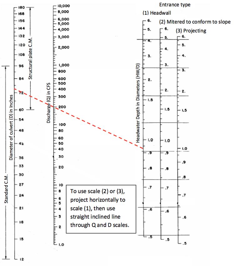
344   APPENDIX A

                   Where: Q100 = predicted peak runoff from a                     2. Easy to use if local rainfall
                   100-year runoff event (in cubic feet second)                      data is available.
                   	           C = runoff coefficient (percent of
                   rainfall that becomes runoff)                             Disadvantages:
                   	           I = uniform rate of rainfall intensity
                   (inches/hour)                                                  1. Flexibility may lead to misuse, or
                   	           A = drainage area (in acres)                          misinterpretation of local conditions.

                   Assumptions:                                                   2. Precipitation factor “I” may be dif-
                                                                                     ficult to obtain in remote areas.
                        1. The 100-year design storm covers the
                           entire basin with uniform constant                     3. Less accurate for watersheds
                           rainfall intensity until the design dis-                  greater than 200 acres
                           charge at the crossing is achieved.
                                                                             Information needed:
                        2. The design watershed charac-
                           teristics are homogenous.                              A = area of watershed (acres)

                        3. Overland flow. This method is                          C = runoff coefficient from Table A-1
                           less accurate or predictable as the
                           percent impervious surface area                        H = elevation difference between
                           in the watershed decreases.                               highest point in watershed and
                                                                                     the crossing point (feet)
                        4. The runoff coefficient (C) is
                           constant across the watershed.                         L = length of channel from the
                                                                                     head of the watershed to the
                        5. The 100-year storm event produces                         crossing point (miles)
                           the 100-year flood flow.
                                                                                  I = uniform rate of rainfall intensity.
                   Advantages:                                                        Obtained from precipitation fre-
                                                                                      quency-duration data for local rain
                        1. Frequently used and flexible enough                        gages as shown in Table A-2.
                           to take into account local conditions.

                    TABLE A-1. Values for Rational Method runoff coefficient (C) values
                                  Soils                       Land use or type                            C value
                                                                    Cultivated                               0.20
                    Sandy and gravelly soils                            Pasture                              0.15
                                                                    Woodland                                 0.10
                                                                    Cultivated                               0.40
                    Loams and similar soils without
                                                                        Pasture                              0.35
                    impeded horizons
                                                                    Woodland                                 0.30

                    Heavy clay soil or those with                   Cultivated                               0.50
                    a shallow impeding horizon;                         Pasture                              0.45
                    shallow over bedrock                            Woodland                                 0.40
CULVERT SIZING PROCEDURES FOR THE 100-YEAR PEAK FLOW 345
TABLE A-2. Example of Rainfall Depth Duration Frequency Data for Eureka, California National Weather
Service Station (NWS)
Design storm Maximum precipitation for indicated rainfall duration
(Return
Period) 5 Min 10 Min 15 Min 30 Min 1 Hr 2 Hr 3 Hr 6 Hr 12 Hr 24 Hr C-Yr
RP 2 0.17 0.25 0.31 0.41 0.55 0.77 0.95 1.34 1.88 2.51 37.88
RP 5 0.23 0.34 0.41 0.55 0.74 1.04 1.28 1.81 2.54 3.38 47.93
RP 10 0.27 0.39 0.48 0.64 0.86 1.21 1.49 2.10 2.95 3.93 53.51
RP 25 0.32 0.46 0.56 0.75 1.00 1.42 1.74 2.45 3.44 4.59 59.83
RP 50 0.35 0.51 0.62 0.82 1.10 1.56 1.92 2.70 3.79 5.06 63.88
RP 100 0.38 0.55 0.67 0.90 1.20 1.70 2.09 2.95 4.13 5.51 67.71
RP 200 0.41 0.59 0.72 0.97 1.30 1.84 2.25 3.18 4.46 5.95 71.30
RP 500 0.45 0.65 0.79 1.06 1.41 2.00 2.46 3.47 4.86 6.49 76.06
RP 1000 0.48 0.69 0.84 1.13 1.51 2.14 2.63 3.70 5.20 6.93 78.94
RP 10000 0.58 0.83 1.01 1.35 1.80 2.55 3.13 4.42 6.21 8.28 88.75
Steps: the crossing point (in feet) (where
the culvert is going to be installed).
1. Select runoff coefficient (C) values:
Several different publications give a (Note: if the value of Tc is calcu-
range of “C” values for the rational lated as less than 10 minutes,
formula, however, the values given in studies suggest you should use
Table A-1 by Rantz (1971) appear to be a default value of 10 minutes)
the most appropriate for the woodlands
and forests around Eureka, California. b. Uniform rate of rainfall intensity.
2. Select a rainfall intensity (I) value: Once the time of concentration has
In selecting an “I” value, two factors been determined, then that value
are considered: a) the travel time is used to determine which rainfall
or time of concentration (Tc) for the duration to use (i.e., if Tc = 1 hour,
runoff to reach the crossing, and b) then use 100-year, 1 hour precipita-
the precipitation conditions for the tion duration; if Tc = 4 hours, then use
particular watershed in question. 100-year, 4-hour duration). Rainfall
depth duration tables similar to Table
a. Time of concentration (Tc) can be A-2 are available for precipitation
calculated using the formula: stations throughout each state. For
0.385 example, rainfall depth duration fre-
Tc =[11.9L3
H ] quency data can be obtained from
the California Department of Water
Where: Tc = time of concentration Resources on-line at ftp://ftp.water.
(in hours) ca.gov/users/dfmhydro/Rainfall%20
L = length of channel in miles from Dept-Duration-Frequency/. Contact your
the head of the watershed to the state’s water resources department (or
crossing point its equivalent) to obtain rainfall depth
H = elevation difference between duration frequency data for your area.
highest point in the watershed and
HANDBOOK FOR FOREST, RANCH AND RURAL ROADS346 APPENDIX A
Example: Rational Method used to the precipitation and runoff data collected
calculate 100-year design storm from more than 700 stream gaging stations in
California (USGS, 2012). For the purposes of
1. Area of example stream crossing this handbook, only the set of equations for the
watershed (A) = 100 acres. 100-year design flood flow are shown below:
2. Runoff coefficient (C) = 0.30 (loam North Coast Q100 = 48.5A0.866p0.556
woodland soil, from Table A-1)
Sierra Q100 = 20.6A0.874p1.24H–0.25
3. Calculate the time of concentration (Tc)
0.385 Desert Region Q100 = 1,350A0.506
Tc = [
11.9L3
H ] Central Coast Q100 = 11.0A0.84p0.994
Where,
South Coast Q100 = 3.28A0.891p1.59
L = 1.8 mi., H = 200 ft.
0.385 Lahontan Q100 = 0.713A0.731p1.56
Tc = [
11.9(1.8)3
200 ] Where:
Q100 = predicted peak runoff from a
= 0.67 inches 100-year storm (cubic feet second)
A = drainage area (square miles)
According to Table A-2, a value H = Mean basin elevation (feet)
of 0.67 inches corresponds to the P = mean annual precipi-
15-minute intensity of a 100-year tation (inches/year)
return period storm event.
Assumptions:
4. Calculate the rainfall intensity (I)
1. The 100-year design storm uniformly
I=( 0.67 in
15 min
× ) (
x in
60 min
= 2.68 in/hr) covers large geographic areas.
5. Calculate Q100 2. The design watershed charac-
teristics are homogenous.
Q100 = CIA
Q100 = (0.3)×(2.68)×(100) 3. The 100-year storm event produces
= 80.4 cubic feet per second (cfs) the 100-year flood flow.
Method 2. THE USGS Advantages:
MAGNITUDE AND FREQUENCY
METHOD FOR ESTIMATING 1. Equations are based on a large set
100-YEAR FLOOD DISCHARGE of widely distributed gaging loca-
tions, including rain on snow events.
The USGS Magnitude and Frequency Method
is based on a set empirical equations derived 2. Easy to use.
for six regions in the state of California for the
2-, 5-, 10-, 25-, 50-, and 100-year design flood 3. Mean basin elevation is easy to deter-
flows. These equations were developed from mine from USGS topographic maps.CULVERT SIZING PROCEDURES FOR THE 100-YEAR PEAK FLOW 347
4. Mean annual precipitation 5. Calculate Q100 for the Sierra Region:
data are readily available
Q100 = 20.6A0.874p1.24H–0.25
5. Equations were updated in 2012. Q100 = 20.6(0.7)0.874651.244,112–0.25
Q100 = 334 cubic feet
Disadvantages: per second (cfs)
1. Generalizes vast geographic areas and Method 3. FLOW
can result in over estimation and under- TRANSFERENCE METHOD
estimation at the local watershed level. FOR ESTIMATING 100-YEAR
FLOOD DISCHARGE
2. Less accurate for watersheds less
than 100 acres. The regression equa- The 100-year design flood flow can also be
tions were based on data for larger calculated for proposed stream crossings
watershed areas (>100 acres), and that are located in or nearby a hydrologically
therefore using the regression equa- similar watershed that has a long-term gaging
tions for smaller watersheds would station. The 100-yr discharge is calculated
result in extrapolating the Q100 estimate by adjusting for the difference in drainage
below the range of data used to area between the gaged station and the
develop the regression equation. ungaged site using the following equation:
b
Information needed: Q100 = Q100g ( )
Au
Ag
1. A = area of watershed (acres) Where:
Q100u = peak runoff from a 100-year
storm at ungaged site (cubic feet per
2. P = mean annual precipitation (in/year) second)
Q100g = peak runoff from a 100-year
3. H = Mean basin elevation (feet). storm at gaged site (cubic feet per
second)
Example: USGS Magnitude and Au = drainage area at ungaged site
Frequency Method used to (square miles)
calculate 100-year design storm Ag = drainage area at gaged site
(square miles)
1. Geographic area = Sierra Nevada b = exponent for drainage area
Region (e.g., Mohawk Ravine in from appropriate USGS Magni-
Nevada County, California) tude and Frequency equation—for
example, the exponent (b) = 0.87
2. Area of example stream for the North Coast USGS Mag-
crossing watershed (A) = 445 nitude and Frequency Method
acres or 0.7 square miles. equation (see Method 2 above)
3. Mean annual precipita- Assumptions:
tion (P) = 65 in/year
1. Ungaged and gaged stream sites have
4. Mean basin elevation (H) = 4,112 feet the same geomorphic and hydrologic
characteristics.
HANDBOOK FOR FOREST, RANCH AND RURAL ROADS348 APPENDIX A
2. Long-term stream gaging 2. Q100u = 14,000 cfs
data at gaged site.
3. Area of example gaged stream
Advantages: crossing watershed (Ag) = 54,000
acres or 84.4 square miles.
1. More accurate than other methods
if the stream gaging station is 4. Area of example ungaged stream
nearby and the available stream crossing watershed (Au) = 300
gaging peak discharge records are acres or 0.47 square miles.
accurate (Cafferata et al., 2004)
5. b = 0.87 – area exponent from
2. Easy to use. the North Coast USGS Magni-
tude and Frequency equation
3. Local data are more likely to reflect
the proposed stream crossing site’s 6. Calculate Q100:
drainage basin characteristics (e.g., b
slopes, geology, soils, and climate). Q100 = Q100g ( )
Au
Ag
0.87
Disadvantages: Q100 = 14,000 cfs ( 0.47 sq mi
84.4 sq mi )
1. Less accurate if gaging data Q100 = 153 cubic feet
record is less than 20 years. per second (cfs)
2. Less accurate if used with gaged and C. SIZING CULVERTS USING
ungaged watersheds that are in differ- THE FEDERAL HIGHWAY
ent locations or have different water- ADMINISTRATION CULVERT
shed conditions and characteristics. CAPACITY NOMOGRAPH
Information needed: The Federal Highway Administration (FHWA)
Culvert Capacity Nomograph is commonly used
1. Au = drainage area at ungaged throughout the U.S. as a tool to determine
site (square miles) the recommended culvert diameter based on
calculated design stream flow and headwater
2. Ag = drainage area at gaged depth (headwall/diameter) ratio (Figure A-1).
site (square miles)
Once the 100-year design flood flow is deter-
3. b = exponent for drainage area mined using one or more of the methods
from appropriate USGS Magnitude stated previously, the steps to determine the
and Frequency Method equation adequate culvert size are very straight forward:
Example: Flow Transference 1. Determine the culvert “entrance
Method used to calculate type” from the three types illustrated
100-year design storm in Figure A-1. Typically, most rural
roads have culverts with “project-
1. Geographic area = North Coast (e.g., ing” (barrel shaped) inlets. Other
unnamed tributary in North Coast)CULVERT SIZING PROCEDURES FOR THE 100-YEAR PEAK FLOW 349
choices include mitered or beveled culvert with Headwater Depth ratio = 1
inlets and culverts with headwalls. would require a 72 in diameter pipe.
2. Determine the “Headwater Depth D. SIZING CULVERTS TO
Ratio” for the proposed stream crossing. ACCOMMODATE THE
The “Headwater Depth Ratio” is the 100-YEAR DESIGN FLOOD
ratio HD/D where HD is the headwall FLOW, WOODY DEBRIS
depth from the height of the fill where AND SEDIMENT
water would begin to spill out of the
crossing (this could be the low point Typically culverts are sized to only accommo-
in the fill or an adjacent road ditch) to date the 100-year design flood flow. Some
the bottom of the culvert invert (culvert landowners and land managers desire to
bottom), and D is the diameter or rise design stream crossing culverts to accommo-
of the culvert inlet. It is not recom- date expected sediment and organic debris in
mended to design a stream crossing transport in addition to meeting the require-
culvert with a HW/D ratio greater ments for passing 100-year peak flows. This is
than 1, even though the fill may be especially important in unconfined and confined
considerably higher and a large pond stream channels that transport a lot of woody
could be physically accommodated.1 debris and sediment during flood flows.
3. To size a projecting inlet culvert, One proposed methodology for accomplish-
place a straight edge connecting the ing this includes designing culvert size based
“Headwater Depth” ratio of 1 on the on 0.67 headwall-to-culvert diameter ratio
“Projecting Inlet” scale at (far right (HW/D), instead of the 1.0 HW/D that is typi-
scale of the nomograph) through cally applied (Cafferata et al., 2004). This often
the 100-year design flood discharge results in culverts that are 12 in. diameter
calculated for the proposed stream larger than would be required to pass the
crossing site (see middle scale on 100-year peak flood flow. Another method to
diagram for “Discharge (Q) in cfs.” reduce the potential for culvert plugging by
sediment and organic debris is to size culverts
4. Read off the needed culvert diameter based on bankfull channel width, either by
on the left scale of the nomograph. using oval or arch culverts, or by employing
oversized round culverts that match or exceed
5. For example, a stream with Q100 = 200 mean bankfull channel width (Flanagan and
cfs, designed with a projecting inlet Furniss, 2003). This is often employed when
designing embedded culverts for fish passage
1 Current recommended design standards are for
culverts to accommodate a “Headwater Depth” ratio (NMFS, 2001). A third method to account for
of 1, where the culvert is assumed to be over capacity if
the water depth rises above the top of the culvert inlet
plugging potential (and which PWA gener-
(HW/D = 1). This is a conservative and protective design ally employs) is to apply secondary treatments,
recommendation. Technically, most stream crossing fills have
room for standing water higher, sometimes a lot higher, such as flared inlets or trash barriers, at cul-
than the top of the culvert, but relying on high headwalls verted stream crossings judged to have a higher
to accommodate peak flows and standing water is a risky
proposition that can lead to increased risk of overtopping than normal likelihood of culvert plugging.
and crossing failure. Because most culvert plugging and
exceedance is attributable to culvert plugging with woody
debris and sediment, proposed HW/D design ratios are
now proposed to be less than 1 (See Section “D” below
for “Headwater Depth” suggestions for accommodating or
accounting for woody debris and sediment).
HANDBOOK FOR FOREST, RANCH AND RURAL ROADS350 APPENDIX A
FIGURE A-1.
FHWA Culvert
Capacity
Inlet Control
Nomograph.CULVERT SIZING PROCEDURES FOR THE 100-YEAR PEAK FLOW 351
E. REFERENCES
Cafferata, P., Spittler, T., Wopat, M., Bundros, Flanagan, S. A.; Furniss. M. J. 1997. Field
G., and Flanagan, S., 2004, Designing indicators of inlet-controlled road-
watercourse crossings for passage of 100 stream-crossing capacity. Gen. Tech.
year flood flows, wood, and sediment, Rep. 9777 1807–SDTDC. San Dimas,
California Department of Forestry CA: U.S. Department of Agriculture,
and Fire Protection, Sacramento, CA. Forest Service, San Dimas Technology
Available at: http://www.fire.ca.gov/ and Development Center. 5 p.
ResourceManagement/PDF/100yr32links.pdf
National Marine Fisheries Service, 2011,
Federal Highway Administration, 1965, Hydraulic Guidelines for salmonid passage at
charts for the selection of highway culverts, stream crossings, Department of
HEC 5, Hydraulic Engineering Circular Commerce, National Oceanic and
No. 5, U.S. Department of Commerce. Atmospheric Administration (NOAA).
Available at: http://www.fhwa.dot.gov/
engineering/hydraulics/pubs/hec/hec05.pdf USGS, 2012, Methods for Determining
Magnitude and Frequency of Floods
in California, Based on Data Through
Water Year 2006, US Geological
Survey Scientific Investigations Report
2012-5113, 38 p. Available at: http://
pubs.usgs.gov/sir/2012/5113/
HANDBOOK FOR FOREST, RANCH AND RURAL ROADSNOTES:
You can also read