Visual modeling with a hand-held camera
←
→
Page content transcription
If your browser does not render page correctly, please read the page content below
Visual modeling with a hand-held camera
                      MARC POLLEFEYS
  Department of Computer Science, University of North Carolina,
                  Chapel Hill, NC 27599-3175
                           marc@cs.unc.edu

LUC VAN GOOL, MAARTEN VERGAUWEN, FRANK VERBIEST,
              KURT CORNELIS AND JAN TOPS
           Center for Processing of Speech and Images,
                 Katholieke Universiteit Leuven,
        Kasteelpark Arenberg 10, B-3001 Leuven, Belgium
                    Luc.VanGool@esat.kuleuven.ac.be

                 Maarten.Vergauwen@esat.kuleuven.ac.be

                   Frank.Verbiest@esat.kuleuven.ac.be

                   Kurt.Cornelis@esat.kuleuven.ac.be

                      Jan.Tops@esat.kuleuven.ac.be

                       REINHARD KOCH
        Institut für Informatik und Praktische Mathematik,
              Christian-Albrechts-Universität Kiel,
       Hermann-Rodewald-Str. 3, D-24098 Kiel, Germany
                     rk@mip.informatik.uni-kiel.de

                                   1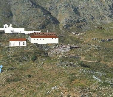
Abstract

         In this paper a complete system to build visual models from camera images is presented.
      The system can deal with uncalibrated image sequences acquired with a hand-held camera.
      Based on tracked or matched features the relations between multiple views are computed.
      From this both the structure of the scene and the motion of the camera are retrieved. The am-
      biguity on the reconstruction is restricted from projective to metric through self-calibration.
      A flexible multi-view stereo matching scheme is used to obtain a dense estimation of the
      surface geometry. From the computed data different types of visual models are constructed.
      Besides the traditional geometry- and image-based approaches, a combined approach with
      view-dependent geometry and texture is presented. As an application fusion of real and
      virtual scenes is also shown.

keywords: Visual modeling, Structure-from-Motion, Projective reconstruction, Self-calibration,
Multi-view stereo matching, Dense reconstruction, 3D reconstruction, Image-based rendering,
Augmented video, hand-held camera.

                                                    2
1 Introduction
During recent years a lot of effort was put in developing new approaches for modeling and
rendering visual scenes. A few years ago the main applications of 3d modeling in vision were
robot navigation and visual inspection. Nowadays however the emphasis has changed. There is
more and more demand for 3D models in computer graphics, virtual reality and communication.
This results in a change in the requirements. The visual quality of the models becomes the main
point of attention. There is an important demand for simple and flexible acquisition procedures.
Therefore calibration should be absent or restricted to a minimum. Many new applications also
require robust low cost acquisition systems. This stimulates the use of consumer photo- or video
cameras.
   In this paper we present an approach that can be used to obtain several types of visual models
from images acquired with an uncalibrated camera. The user acquires the images by freely
moving the camera around an object or scene. Neither the camera motion nor the camera settings
have to be known a priori. The presented approach can generate a textured 3D surface model or
alternatively render new views using a combined geometry- and image-based approach that uses
view-dependent texture and geometry. The system can also be used to combine virtual objects
with real video, yielding augmented video sequences.
   Other approaches for extracting 3D shape and texture from image sequences acquired with
a freely moving camera have been proposed. The approach of Tomasi and Kanade [59] used an
affine factorization method to extract 3D from image sequences. An important restriction of this
system is the assumption of orthographic projection. Another type of approach starts from an
approximate 3D model and camera poses and refines the model based on images (e.g. Facade
proposed by Debevec et al. [8]). The advantage is that less images are required. On the other
hand a preliminary model must be available which mostly limits the approach to man-made
environments. This approach also combines geometry- and image-based techniques, however
only the texture is view-dependent.
   The approach presented here combines many ideas and algorithms that have been developed
in recent years. This paper aims at consolidating these results by bringing them together and

                                               3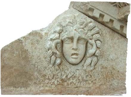
showing how they can be combined to yield a complete visual modeling approach. In Sec-
tion 1.1 notations and background are given. The rest of the paper is then organized as follows.
Section 2 discusses feature extraction and matching and the computation of the multi-view re-
lations. Section 3 deals with the structure and motion recovery, including self-calibration. In
Section 4 the approach to obtain dense depth maps is presented and in Section 5 the construction
of the different visual models is discussed. The paper is concluded in Section 6.

1.1 Notations and background

In this section we briefly introduce some of the geometric concepts used throughout the paper.
A more in depth description can be found in [23, 13]. A perspective camera is modeled through
the projection equation
                                                                                                    (1)

where     represents the equality up to a non-zero scale factor,  is a 4-vector that represents 3D
world point in homogeneous coordinates, similarly is a 3-vector that represents a corresponding
2D image point and        is a      projection matrix.   In a metric or Euclidean frame         can be
factorized as follows


                                       - where

                                                                                                    (2)


contains the intrinsic camera parameters,  is a rotation matrix representing the orientation and
is a 3-vector representing the position of the camera. The intrinsic camera parameter        represents
the focal length measured in width of pixels,  is the aspect ratio of pixels,    represent the
coordinates of the principal point and  is a term accounting for the skew. In general  can be
assumed zero. In practice, the principal point is often close to the center of the image and the
aspect ratio  close to one. In many cases the camera does not perfectly satisfy the perspective
projection model and distortions have to be taken into account, the most important being radial
distortion. In practice, it is often sufficient to model the radial distortion as follows:

                    - with
                                                                                            (3)

                                                   4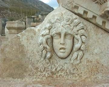
where  indicates the amount of radial distortion that is present in the image. For high accuracy
applications more advanced models can be used [68, 54].
    In this paper the notation    will be used to indicate the Euclidean distance between
entities in the images.

two view geometry         The point  corresponding to the point                         in another image is bound to be
on the projection of its line of sight                 where  is the fundamental matrix for the two views
under consideration. Therefore, the following equation should be satisfied for all corresponding
points:
                                                                                                                    (4)

The fundamental matrix has rank 2 and the right and left null-space of                                 corresponds to the
epipoles. The epipoles  and  are the projections of the projection center of one image in the
other image. The fundamental matrix can be obtained from two projection matrices                                 and    as

                                                                                                                 (5)

where the epipole          with  the solution of               .

Homographies These can be used to transfer image points that corresponds to 3D points that
are on a specific plane from one image to the other, i.e.                                   where    is the homography
that corresponds to that plane (for the two views under consideration). There is an important
relationship between such homographies and the fundamental matrix:

                                         and                                                        (6)

with   an anti-symmetric matrix representing the vector product with the epipole and with
a vector related to the plane. Homographies for a plane                                 can also be obtained from
projection matrices as


                                ¼         ¼      with       ¼         ¼                                       (7)


From 3 points    and  a plane is obtained as the right null space of      .

                                                              5
comparing images regions Image regions are typically compared using sum-of-square-differences
(SSD) or zero-mean normalized cross-correlation (ZNCC). Consider a window  in image  and
a corresponding region   in image  . The dissimilarity between two image regions based
on SSD is given by

                                                                        (8)


where    is a weighting function that is defined over W. Typically,      or it is a
Gaussian. The similarity measure between two image regions based on ZNCC is given by


                                                                                                 (9)


with

                              and
                                                              the mean image intensity in the
considered region. Note that this last measure is invariant to global intensity and contrast changes
over the considered regions.

2 Relating images
Starting from a collection of images or a video sequence the first step consists in relating the
different images to each other. This is not an easy problem. A restricted number of corresponding
points is sufficient to determine the geometric relationship or multi-view constraints between
the images. Since not all points are equally suited for matching or tracking (e.g. a pixel in a
homogeneous region), the first step consist of selecting a number of interesting points or feature
points. Some approaches also use other features, such as lines or curves, but these will not be
discussed here. Depending on the type of image data (i.e. video or still pictures) the feature
points are tracked or matched and a number of potential correspondences are obtained. From
these the multi-view constraints can be computed. However, since the correspondence problem
is an ill-posed problem, the set of corresponding points can be contaminated with an important
number of wrong matches or outliers. In this case, a traditional least-squares approach will fail
and therefore a robust method is needed. Once the multi-view constraints have been obtained

                                                    6
they can be used to guide the search for additional correspondences. These can then be used to
further refine the results for the multi-view constraints.

2.1 Feature extraction and matching

One of the most important requirements for a feature point is that it can be differentiated from its
neighboring image points. If this were not the case, it wouldn’t be possible to match it uniquely
with a corresponding point in another image. Therefore, the neighborhood of a feature should be
sufficiently different from the neighborhoods obtained after a small displacement.
   A second order approximation of the dissimilarity, as defined in Eq. (8), between a image
window  and a slightly translated image window is given by


                                              with


                                                                                                         (10)
To ensure that no displacement exists for which  is small, the eigenvalues of  should both
be large. This can be achieved by enforcing a minimal value for the smallest eigenvalue [53] or
alternatively for the following corner response function                     trace   [17] where
 is a parameter set to 0.04 (a suggestion of Harris). In the case of tracking this is sufficient to
ensure that features can be tracked from one video frame to the next. In this case it is natural
to use the tracking neighborhood to evaluate the quality of a feature (e.g. a    window with
    ). Tracking itself is done by minimizing Eq. 8 over the parameters of               . For small
steps a translation is sufficient for   .   To evaluate the accumulated difference from the start of
the track it is advised to use an affine motion model.
   In the case of separate frames as obtained with a still camera, there is the additional re-
quirement that as much image points originating from the same 3D points as possible should
be extracted. Therefore, only local maxima of the corner response function are considered as
suitable features. Sub-pixel precision can be achieved through quadratic approximation of the
neighborhood of the local maxima. A typical choice for   in this case is a Gaussian with
     . Matching is typically done by comparing small, e.g.   , windows centered around

                                                     7
the feature through SSD or ZNCC. This measure is only invariant to image translations and can
therefore not cope with too large variations in camera pose.
   To match images that are more widely separated, it is required to cope with a larger set of
image variations. Exhaustive search over all possible variations is computationally intractable. A
more interesting approach consists of extracting a more complex feature that not only determines
the position, but also the other unknowns of a local similarity [51] or affine transformation [36,
65].

2.2 Two view geometry computation

Even for an arbitrary geometric structure, the projections of points in two views contain some
structure. Finding back this structure is not only interesting to retrieve information on the relative
pose between the two views [11, 18], but also to eliminate mismatches and to facilitate the
search for additional matches. This structure is corresponds to the epipolar geometry and is
mathematically expressed by the fundamental matrix. Given a number of corresponding points
Eq. (4) can be used to compute . This equation can be rewritten in the following form:

                                                                                  (11)

with             and           a vector containing the elements of the fundamental
matrix. Stacking 8 or more of these equations allows to linearly solve for the fundamental matrix.
Even for 7 corresponding points the one parameter family of solutions obtained by solving the
linear equations can be restricted to 1 or 3 solutions by enforcing the cubic rank-2 constraint
             . As pointed out by Hartley [20] it is important to normalize the image
coordinates before solving the linear equations. Otherwise the columns of Eq. (11) would differ
by several orders of magnitude and the error would concentrate on the coefficients corresponding
to the smaller columns. This normalization can be achieved by transforming the image center
to the origin and scaling the images so that the coordinates have a standard deviation of unity.
More advanced approaches have been proposed, e.g. [37], but in practice the simple approach is
sufficient to initialize a non-linear minimization. The result of the linear equations can be refined

                                                   8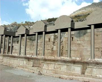
by minimizing the following criterion [69]:

                                                                               (12)

This criterion can be minimized through a Levenberg-Marquard algorithm [47]. An even better
approach consists of computing a maximum-likelihood estimation (MLE) by minimizing the
following criterion:

                                               with                   (13)

Although in this case the minimization has to be carried out over a much larger set of vari-
ables, this can be achieved efficiently by taking advantage of the sparsity of the problem (see
Section 3.3).
   To compute the fundamental matrix from a set of matches that were automatically obtained
from a pair of real images, it is important to explicitly deal with outliers. If the set of matches
is contaminated with even a small set of outliers, the result of the above method can become
unusable. This is typical for all types of least-squares approaches (even non-linear ones). The
problem is that the quadratic penalty (which is optimal for Gaussian noise) allows for a single
outlier that is very far away from the true solution to completely bias the final result.
   The approach that is used to cope with this problem is the RANSAC algorithm that was
proposed by Fischler and Bolles [14]. A minimal subset of the data is randomly selected and
the solution obtained from it is used to segment the remainder of the dataset in “inliers” and
“outliers”. If the initial set contains no outliers, it can be expected that an important number
of inliers will support the solution, otherwise the initial subset is probably contaminated with
outliers. This procedure is repeated until a satisfying solution is obtained. This can for example
be defined as a probability in excess of  that a good subsample was selected. The expression
for this probability is          with  the fraction of inliers, and  the number of
features in each sample and  the number of trials (see Rousseeuw [48]).
   Once the epipolar geometry has been computed it can be used to guide the matching pro-
cedure toward additional matches. At this point only features that are close to the epipolar line
should be considered for matching. Table 1 summarizes the robust approach to the determination
of the two-view geometry.

                                                      9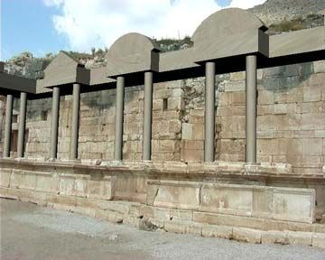
Step 1. Compute a set of potential matches

                         Step 2. While      do

                              step 2.1 select minimal sample (7 matches)

                              step 2.2 compute solutions for F

                              step 2.3 determine inliers

                         step 3. Refine F based on all inliers

                         step 4. Look for additional matches

                         step 5. Refine F based on all correct matches

             Table 1: Overview of the two-view geometry computation algorithm.

3 Structure and motion recovery
In the previous section it was seen how different views could be related to each other. In this
section the relation between the views and the correspondences between the features will be
used to retrieve the structure of the scene and the motion of the camera. This problem is called
Structure and Motion.
   The approach that is proposed here extends [1, 30] by being fully projective and therefore
not dependent on the quasi-euclidean initialization. This was achieved by carrying out all mea-
surements in the images. This approach provides an alternative for the triplet-based approach
proposed in [15]. An image-based measure that is able to obtain a qualitative distance between
viewpoints is also proposed to support initialization and determination of close views (indepen-
dently of the actual projective frame).
   At first two images are selected and an initial reconstruction frame is set-up. Then the pose of
the camera for the other views is determined in this frame and each time the initial reconstruction
is refined and extended. In this way the pose estimation of views that have no common features

                                                10
with the reference views also becomes possible. Typically, a view is only matched with its
predecessor in the sequence. In most cases this works fine, but in some cases (e.g. when the
camera moves back and forth) it can be interesting to also relate a new view to a number of
additional views. Once the structure and motion has been determined for the whole sequence,
the results can be refined through a projective bundle adjustment. Then the ambiguity will be
restricted to metric through self-calibration. Finally, a metric bundle adjustment is carried out to
obtain an optimal estimation of the structure and motion.
3.1 Initial structure and motion
The first step consists of selecting two views that are suited for initializing the sequential structure
and motion computation. On the one hand it is important that sufficient features are matched
between these views, on the other hand the views should not be too close to each other so that the
initial structure is well-conditioned. The first of these criteria is easy to verify, the second one is
harder in the uncalibrated case. The image-based distance that we propose is the median distance
between points transferred through an average planar-homography and the corresponding points
in the target image:
median (14)
This planar-homography H is determined as follows from the matches between the two views:
with argmin (15)
In practice the selection of the initial frame can be done by maximizing the product of the number
of matches and the image-based distance defined above. When features are matched between
sparse views, the evaluation can be restricted to consecutive frames. However, when features
are tracked over a video sequence, it is important to consider views that are further apart in the
sequence.
In the case of a video sequence where consecutive frames are very close together the com-
putation of the epipolar geometry is ill conditioned. To avoid this problem we propose to only
consider properly selected key-frames for the structure and motion recovery. If it is important to
11compute the motion for all frames, such as for insertion of virtual objects in a video sequence
(see Section 5.3), the pose for in-between frames can be computed afterward. We propose to
use model selection [61] to select the next key-frame only once the epipolar geometry model
explains the tracked features better than the simpler homography model 1 .
Initial frame Two images of the sequence are used to determine a reference frame. The world
frame is aligned with the first camera. The second camera is chosen so that the epipolar geometry
corresponds to the retrieved :
(16)
Eq. (16) is not completely determined by the epipolar geometry (i.e. and ), but has 4 more
degrees of freedom (i.e. and ). determines the position of the reference plane (i.e. the plane
at infinity in an affine or metric frame) and determines the global scale of the reconstruction.
The parameter can simply be put to one or alternatively the baseline between the two initial
views can be scaled to one. In [1] it was proposed to set the coefficient of to ensure a quasi-
Euclidean frame, to avoid too large projective distortions. This was needed because not all parts
of the algorithms where strictly projective. For the structure and motion approach proposed in
this paper can be arbitrarily set, e.g. .
Initializing structure Once two projection matrices have been fully determined the matches
can be reconstructed through triangulation. Due to noise the lines of sight will not intersect
perfectly. In the uncalibrated case the minimizations should be carried out in the images and not
in projective 3D space. Therefore, the distance between the reprojected 3D point and the image
points should be minimized:
(17)
1
In practice, to avoid selecting too many key-frames, we propose to pick a key-frame at the last frame for which
with the number of valid tracks and the number of valid tracks when the epipolar geometry model
overtakes the homography model.
12It was noted by Hartley and Sturm [21] that the only important choice is to select in which
epipolar plane the point is reconstructed. Once this choice is made it is trivial to select the
optimal point from the plane. A bundle of epipolar planes has only one parameter. In this case
the dimension of the problem is reduced from 3-dimensions to 1-dimension. Minimizing the
following equation is thus equivalent to minimizing equation (17).
(18)
with and the epipolar lines obtained in function of the parameter describing the
bundle of epipolar planes. It turns out (see [21]) that this equation is a polynomial of degree 6 in
. The global minimum of equation (18) can thus easily be computed. In both images the point
on the epipolar line and closest to the points resp. is selected. Since these
points are in epipolar correspondence their lines of sight meet in a 3D point.
3.2 Updating the structure and motion
The previous section dealt with obtaining an initial reconstruction from two views. This sec-
tion discusses how to add a view to an existing reconstruction. First the pose of the camera is
determined, then the structure is updated based on the added view and finally new points are
initialized.
projective pose estimation For every additional view the pose toward the pre-existing recon-
struction is determined, then the reconstruction is updated. This is illustrated in Figure 1. The
first step consists of finding the epipolar geometry as described in Section 2.2. Then the matches
which correspond to already reconstructed points are used to infer correspondences between 2D
and 3D. Based on these the projection matrix is computed using a robust procedure similar to
the one laid out in Table 1. In this case a minimal sample of 6 matches is needed to compute .
A point is considered an inlier if there exists a 3D point that projects sufficiently close to all as-
sociated image points. This requires to refine the initial solution of based on all observations,
including the last. Because this is computationally expensive (remember that this has to be done
for each generated hypothesis), it is advised to use a modified version of RANSAC that cancels
13M
mi−3
^ i−3 mi−2 mi−1
m ^ i−2 F mi
m ^
m ^
mi
i−1
Figure 1: Image matches ( ) are found as described before. Since the image points, ,
relate to object points, , the pose for view can be computed from the inferred matches ( ).
A point is accepted as an inlier if a solution for
exist for which !
for each view
in which has been observed.
14the verification of unpromising hypothesis [4]. Once ! has been determined the projection of
already reconstructed points can be predicted, so that some additional matches can be obtained.
This means that the search space is gradually reduced from the full image to the epipolar line to
the predicted projection of the point.
This procedure only relates the image to the previous image. In fact it is implicitly assumed
that once a point gets out of sight, it will not come back. Although this is true for many sequences,
this assumptions does not always hold. Assume that a specific 3D point got out of sight, but that
it is visible again in the last two views. In this case a new 3D point will be instantiated. This
will not immediately cause problems, but since these two 3D points are unrelated for the system,
nothing enforces their position to correspond. For longer sequences where the camera is moved
back and forth over the scene, this can lead to poor results due to accumulated errors.
The solution that we propose is to match all the views that are close with the actual view
(as described in Section 2.2). For every close view a set of potential 2D-3D correspondences is
obtained. These sets are merged and the camera projection matrix is estimated using the same
robust procedure as described above, but on the merged set of 2D-3D correspondences [30, 49].
Close views are determined as follows. First a planar-homography that explains best the
image-motion of feature points between the actual and the previous view is determined (using
Eq. 15). Then, the median residual for the transfer of these features to other views using homo-
graphies corresponding to the same plane are computed (see Eq. (14)). Since the direction of the
camera motion is given through the epipoles, it is possible to limit the selection to the closest
views in each direction. In this case it is important to take orientation into account [22, 33] to
differentiate between opposite directions.
Refining and extending structure The structure is refined using an iterated linear reconstruc-
tion algorithm on each point. Eq. (1) can be rewritten to become linear in :
(19)
with the -th row of and being the image coordinates of the point. An estimate
of is computed by solving the system of linear equations obtained from all views where a
15
corresponding image point is available. To obtain a better solution the criterion
should be minimized. This can be approximately obtained by iteratively solving the following
weighted linear equations (in matrix form):


                                                                                            (20)


where  is the previous solution for . This procedure can be repeated a few times. By solving
this system of equations through SVD a normalized homogeneous point is automatically ob-
tained. If a 3D point is not observed the position is not updated. In this case one can check if
the point was seen in a sufficient number of views to be kept in the final reconstruction. This
minimum number of views can for example be put to three. This avoids to have an important
number of outliers due to spurious matches.
      Of course in an image sequence some new features will appear in every new image. If point
matches are available that were not related to an existing point in the structure, then a new point
can be initialized as in section 3.1.

      After this procedure has been repeated for all the images, one disposes of camera poses for all
the views and the reconstruction of the interest points. In the further modules mainly the camera
calibration is used. The reconstruction itself is used to obtain an estimate of the disparity range
for the dense stereo matching.

3.3 Refining structure and motion

Once the structure and motion has been obtained for the whole sequence, it is recommended to
refine it through a global minimization step. A maximum likelihood estimation can be obtained
through bundle adjustment [63, 54]. The goal is to find the parameters of the camera view
and the 3D points  for which the mean squared distances between the observed image points
     and the reprojected image points       is minimized. The camera projection model should
also take radial distortion into account. For  views and  points the following criterion should

                                                     16
be minimized:
(21)
If the errors on the localization of image features are independent and satisfy a zero-mean Gaus-
sian distribution then it can be shown that bundle adjustment corresponds to a maximum like-
lihood estimator. This minimization problem is huge, e.g. for a sequence of 20 views and 100
points/view, a minimization problem in more than 6000 variables has to be solved (most of
them related to the structure). A straight-forward computation is obviously not feasible. How-
ever, the special structure of the problem can be exploited to solve the problem much more
efficiently [63, 54]. The key reason for this is that a specific residual is only dependent on one
point and one camera, which results in a very sparse structure for the normal equations.
To conclude this section an overview of the algorithm to retrieve structure and motion from
a sequence of images is given. Two views are selected and a projective frame is initialized.
The matched corners are reconstructed to obtain an initial structure. The other views in the
sequence are related to the existing structure by matching them with their predecessor. Once this
is done the structure is updated. Existing points are refined and new points are initialized. When
the camera motion implies that points continuously disappear and reappear it is interesting to
relate an image to other close views. Once the structure and motion has been retrieved for the
whole sequence, the results can be refined through bundle adjustment. The whole procedure is
summarized in Table 2.
3.4 Upgrading to metric
The reconstruction obtained as described in the previous sections is only determined up to an
arbitrary projective transformation. This might be sufficient for some robotics or inspection
applications, but certainly not for visualization. Therefore we need a method to upgrade the re-
construction to a metric one (i.e. determined up to an arbitrary Euclidean transformation and a
scale factor). This can be done by imposing some constraints on the intrinsic camera parameters.
This approach that is called self-calibration has received a lot of attention in recent years. Mostly
17Step 1. Match or track points over the whole image sequence.
Step 2. Initialize the structure and motion recovery
step 2.1. Select two views that are suited for initialization.
step 2.2. Relate these views by computing the two view geometry.
step 2.3. Set up the initial frame.
step 2.4. Reconstruct the initial structure.
Step 3. For every additional view
step 3.1. Infer matches to the structure and compute the camera
pose using a robust algorithm.
step 3.2. Refine the existing structure.
step 3.3. (optional) For already computed views which are “close”
3.4.1. Relate this view with the current view by finding fea-
ture matches and computing the two view geometry.
3.4.2. Infer new matches to the structure based on the com-
puted matches and add these to the list used in step 3.1.
Refine the pose from all the matches using a robust algorithm.
step 3.5. Initialize new structure points.
Step 4. Refine the structure and motion through bundle adjustment.
Table 2: Overview of the projective structure and motion algorithm.
18self-calibration algorithms are concerned with unknown but constant intrinsic camera parame-
ters [12, 19, 45, 25, 62]. Some algorithms for varying intrinsic camera parameters have also been
proposed [44, 26]. In some cases the motion of the camera is not general enough to allow for
self-calibration to uniquely recover the metric structure and an ambiguity remains. More details
can be found in [56] for constant intrinsics and in [57, 41, 27] for varying intrinsics.
The approach that is presented here was originally proposed in [42] and later adapted to take
a priori information on the intrinsic camera parameters into account which reduces the problem
of critical motion sequences.
The image of the absolute conic One of the most important concepts for self-calibration is
the absolute conic and its projection in the images. The simplest way to represent the ab-
solute conic is through the dual absolute quadric [62]. In a Euclidean coordinate frame
diag and one can easily verify that it is invariant to similarity transforma-
tions. Inversely, it can also be shown that a transformation that leaves the dual quadric
diag unchanged is a similarity transformation. For a projective reconstruction can
be represented by a rank-3 symmetric positive semi-definite matrix. According to the
properties mentioned above a transformation that transforms diag will bring
the reconstruction within a similarity transformation of the original scene, i.e. yield a metric
reconstruction.
The projection of the dual absolute quadric in the image is described by the following equa-
tion:
" (22)
It can be easily verified that in a Euclidean coordinate frame the image of the absolute quadric is
directly related to the intrinsic camera parameters:
" (23)
Since the images are independent of the projective basis of the reconstruction, Eq. (23) is always
valid and constraints on the intrinsics can be translated to constraints on .
19linear self-calibration The approach proposed in this paper is inspired from [42], however,
some important improvements were made. A priori knowledge about the parameters is in-
troduced in the linear computations [46]. This reduces the problems with critical motion se-
quences [56, 41].
The first step consists of normalizing the projection matrices. The following normalization
is proposed:
#
with #
(24)
where and # are the width, resp. height of the image. After the normalization the focal length
should be of the order of unity and the principal point should be close to the origin. The above
normalization would scale a focal length of a 60mm lens to 1 and thus focal lengths in the range
of 20mm to 180mm would end up in the range $ . The aspect ratio is typically also around 1
and the skew can be assumed 0 for all practical purposes. Making these a priori knowledge more
explicit and estimating reasonable standard deviations one could for example get ,
, and . It is now interesting to investigate the impact of this
knowledge on " :
"
(25)
$"
and " . The constraints on the left-hand side of Eq. (22) should also be verified
on the right-hand side (up to scale). The uncertainty can be take into account by weighting the
equations accordingly.
! ! ! !
! ! ! !
! ! ! !
(26)
! !
! !
! !
20with ! the th row of ! with
and % a scale factor that is initially set to 1 and later on to !
the result of the previous iteration. Since is a symmetric matrix it is parametrized
through 10 coefficients. An estimate of the dual absolute quadric can be obtained by solving
the above set of equations for all views through linear least-squares. The rank-3 constraint should
be imposed by forcing the smallest singular value to zero. This scheme can be iterated until the
% factors converge (typically after a few iterations). In most cases, however, the first iteration
is sufficient to initialize the metric bundle adjustment. The upgrading transformation can be
obtained from diag by decomposition of .
The metric structure and motion is then obtained as
and (27)
refinement This initial metric reconstruction should then further be refined through bundle
adjustment to obtain the best possible results. While some approaches suggest an intermediate
non-linear refinement of the self-calibration, our experience shows that this is in general not
necessary of one uses the self-calibration approach presented in the previous paragraph (as well
as an initial correction of the radial distortion). For this bundle adjustment procedure the cam-
era projection model should explicitly represent the constraints on the camera intrinsics. These
constraints can both be hard constraints (imposed through parametrization) or soft constraints
(imposed by including an additional term in the minimization criterion). A good typical choice
of constraints for a photo camera consists of imposing a constant focal length (if no zoom was
used), a constant principal point and radial distortion, an aspect ratio of one and the absence of
skew. However, for a camcorder/video camera it is important to estimate the (constant) aspect
ratio as this can significantly differ from one.
4 Dense surface estimation
With the camera calibration given for all viewpoints of the sequence, we can proceed with meth-
ods developed for calibrated structure from motion algorithms. The feature tracking algorithm
already delivers a sparse surface model based on distinct feature points. This however is not
21sufficient to reconstruct geometrically correct and visually pleasing surface models. This task is
accomplished by a dense disparity matching that estimates correspondences from the images by
exploiting additional geometrical constraints. The dense surface estimation is done in a number
of steps. First image pairs are rectified to the standard stereo configuration. Then disparity maps
are computed through a stereo matching algorithm. Finally a multi-view approach integrates the
results obtained from several view pairs.
4.1 Rectification
Since the calibration between successive image pairs was computed, the epipolar constraint that
restricts the correspondence search to a 1-D search range can be exploited. Image pairs are
warped so that epipolar lines coinciding with the image scan lines. The correspondence search
is then reduced to a matching of the image points along each image scan-line. This results
in a dramatic increase of the computational efficiency of the algorithms by enabling several
optimizations in the computations.
For some motions (i.e. when the epipole is located in the image) standard rectification based
on planar homographies is not possible and a more advanced procedure should be used. The ap-
proach used in the presented system was proposed in [43]. The method combines simplicity with
minimal image size and works for all possible motions. The key idea is to use polar coordinates
with the epipole as origin. Corresponding lines are given through the epipolar geometry. By tak-
ing the orientation [33] into account the matching ambiguity is reduced to half epipolar lines. A
minimal image size is achieved by computing the angle between two consecutive epipolar lines
that correspond to rows in the rectified images to have the worst case pixel on the line preserve
its area. To avoid image degradation, both correction of radial distortion and rectification are
performed in a single resampling step.
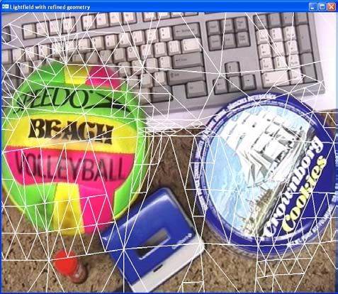
Some examples A first example comes from the castle sequence. In Figure 2 an image pair
and the associated rectified image pair are shown. A second example was filmed with a hand-
held digital video camera in the Béguinage in Leuven. Due to the narrow streets only forward
22Figure 2: Original image pair (left) and rectified image pair (right).
motion is feasible. In this case the full advantage of the polar rectification scheme becomes
clear since this sequence could not have been handled through traditional planar rectification.
An example of a rectified image pair is given in Figure 3. Note that the whole left part of the
rectified images corresponds to the epipole. On the right side of this figure a model that was
obtained by combining the results from several image pairs is shown.
4.2 Stereo matching
The goal of a dense stereo algorithm is to compute corresponding pixel for every pixel of an
image pair. After rectification the correspondence search is limited to corresponding scanlines.
As illustrated in Fig 4, finding the correspondences for a pair of scanlines can be seen as a path
search problem. Besides the epipolar geometry other constraints, like preserving the order of
neighboring pixels, bidirectional uniqueness of the match, and detection of occlusions can be
exploited. In most cases it is also possible to limit the search to a certain disparity range (an
estimate of this range can be obtained from the reconstructed 3D feature points). Besides these
constraints, a stereo algorithm should also take into account the similarity between correspond-
ing points and the continuity of the surface. It is possible to compute the optimal path taking all
the constraints into account using dynamic programming [6, 10, 66]. While many other stereo
approaches are available, we use this one because it provides a good trade-off between quality
and speed. Computation of a disparity map between two video frame with a disparity range of
hundred, including polar rectification, takes less than a minute on a PC. By treating pixels inde-
pendently stereo can be performed much faster (even real-time), but at the expense of quality.
23Figure 3: Rectified image pair (left) and some views of the reconstructed street model (right).
24epipolar line image l
search
region
4
1 4 occlusion
image k
3
2 3
occlusion
1,2 image l
h
at
1 2 3,4 1,2 3 4
p
al
tim
op
Pk Pk+1 1 2 3,4 epipolar line image k
Figure 4: Illustration of the ordering constraint (left), dense matching as a path search problem
(right).
Some recent stereo approaches perform a global optimization that also takes continuity across
scanlines into account and therefore achieve better results, but are much slower. A good taxon-
omy of stereo algorithms can be found in [50]. Notice that because of the modular design of our
3D reconstruction pipeline, it is simple to substitute one stereo algorithm for another.
4.3 Multi-view linking
The pairwise disparity estimation allows to compute image to image correspondence between
adjacent rectified image pairs, and independent depth estimates for each camera viewpoint. An
optimal joint estimate is achieved by fusing all independent estimates into a common 3D model.
The fusion can be performed in an economical way through controlled correspondence linking
(see Figure 5). A point is transferred from one image to the next image as follows:
(28)
with and functions that map points from the original image into the rectified image
and a function that corresponds to the disparity map. When the depth obtained from the
new image point is outside the confidence interval the linking is stopped, otherwise the result
is fused with the previous values through a Kalman filter. This approach is discussed into more
detail in [29]. This approach combines the advantages of small baseline and wide baseline stereo.
25Lk Lk
outlier
ek+1 en e k+1
P1 Pn
P1 PN
... ...
... ...
Pk-2 Pi+2 link terminates
Pk-2 Pk+2
Pk-1 Pk+1
Pk
11
00 Pk+1
Downward linking 00
11 upward linking Pk-1
Pk
Figure 5: Depth fusion and uncertainty reduction from correspondence linking (left), linking
stops when an outlier is encountered (right).
It can provide a very dense depth map by avoiding most occlusions. The depth resolution is
increased through the combination of multiple viewpoints and large global baseline while the
matching is simplified through the small local baselines. Due to multiple observations of a single
surface points the texture can be enhanced and noise and highlights can be removed.
Starting from the computed structure and motion alternative approaches such as sum-of-sum-
of-square-differences (SSSD) [40] or space-carving [32] could also be used. The advantages
of an approach that only uses pairwise matching followed by multi-view linking, is that it is
more robust to changes in camera exposure, non-Lambertian surfaces, passers-by, etc. This is
important for obtaining good quality results using hand-held camera sequences recorded in an
uncontrolled environment.
Some results The quantitative performance of correspondence linking can be tested in differ-
ent ways. One measure already mentioned is the visibility of an object point. In connection
with correspondence linking, we have defined visibility & as the number of views linked to the
reference view. Another important feature of the algorithm is the density and accuracy of the
depth maps. To describe its improvement over the 2-view estimator, we define the fill rate '
and the average relative depth error ( as additional measures. The 2-view disparity estimator
265 5
4 4
3 3
E [%]
E [%]
2 2
1 1
0 0
2 3 5 7 9 11 13 15 2 3 4 5
10 100
8 80
V [view]
6 60
F [%]
4 40
2 20
0 0
2 3 5 7 9 11 13 15 2 3 4 5
N [view] Vmin [view]
Figure 6: Statistics of the castle sequence. Influence of sequence length ) on visibility & and
relative depth error ( . (left) Influence of minimum visibility & on fill rate ' and depth error (
for ) (center). Depth map (above: dark=near, light=far) and error map (below: dark=large
error, light=small error) for ) and & (right).
is a special case of the proposed linking algorithm, hence both can be compared on an equal
basis. Figure 6 displays visibility and relative depth error for sequences from 2 to 15 images of
the castle sequence, chosen symmetrically around the reference image. The average visibility &
shows that for up to 5 images nearly all images are utilized. For 15 images, at average 9 images
are linked. The amount of linking is reflected in the relative depth error that drops from 5% in
the 2 view estimator to about 1.2% for 15 images.
Linking two views is the minimum case that allows triangulation. To increase the reliability
of the estimates, a surface point should be observed in more than two images. We can therefore
impose a minimum visibility & on a depth estimate. This will reject unreliable depth estimates
effectively, but will also reduce the fill rate of the depth map. The graphs in figure 6(center)
show the dependency of the fill rate and depth error on minimum visibility for the sequence
length N=11. The fill rate drops from 92% to about 70%, but at the same time the depth error is
reduced to 0.5% due to outlier rejection. The depth map and the relative error distribution over
the depth map is displayed in Figure 6(right). The error distribution shows a periodic structure
27that in fact reflects the quantization uncertainty of the disparity resolution when it switches from
one disparity value to the next.
5 Visual scene representations
In the previous sections a dense structure and motion recovery approach was given. This yields
all the necessary information to build different types of visual models. In this section several
types of models will be considered. First, the construction of texture-mapped 3D surface models
is discussed. Then, a combined image- and geometry-based approach is presented that can render
models ranging from pure plenoptic to view-dependent texture and geometry models. Finally,
the possibility of fusion of real and virtual scenes in video is also treated. These different cases
will now be discussed in more detail.
5.1 3D surface reconstruction
The 3D surface is approximated by a triangular mesh to reduce geometric complexity and to
tailor the model to the requirements of computer graphics visualization systems. A simple ap-
proach consists of overlaying a 2D triangular mesh on top of one of the images and then build a
corresponding 3D mesh by placing the vertices of the triangles in 3D space according to the val-
ues found in the corresponding depth map. To reduce noise it is recommended to first smooth the
depth image (the kernel can be chosen of the same size as the mesh triangles). The image itself
can be used as texture map (the texture coordinates are trivially obtained as the 2D coordinates
of the vertices).
It can happen that for some vertices no depth value is available or that the confidence is too
low. In these cases the corresponding triangles are not reconstructed. The same happens when
triangles are placed over discontinuities. This is achieved by selecting a maximum angle between
the normal of a triangle and the line-of-sight through its center (e.g. 85 degrees). This simple
approach works very well on the dense depth maps as obtained through multi-view linking. The
surface reconstruction approach is illustrated in Figure 7. The texture can be enhanced through
28Figure 7: Surface reconstruction approach (top): A triangular mesh is overlaid on top of the
image. The vertices are back-projected in space according to the depth values. From this a 3D
surface model is obtained (bottom)
the multi-view linking scheme. A median or robust mean of the corresponding texture values is
computed to discard imaging artifacts like sensor noise, specular reflections and highlights[39].
Ideally, to avoid artifacts on stretched triangles (such as the ground in Fig. 7) projective texture
mapping has to be used in stead of the standard affine mapping [9].
To reconstruct more complex shapes it is necessary to combine results from multiple depth
maps. The simplest approach consists of generating separate models independently and then
loading them together in the graphics system. Since all depth-maps can be located in a single
metric frame, registration is not an issue. For more complex scenes different meshes can be
integrated into a single surface representation. Different approaches have been proposed to deal
with this problem. These can broadly be classified in surface-based approaches [64, 55] and
29volumetric approaches [7, 67]. In our approach we have implemented [7] to obtain an implicit
representation of the surface, followed by the marching cubes algorithm to obtain an explicit
mesh representation [35] and finally we apply a variant of [52] to simplify the mesh.
Example A first example was recorded using a consumer camcorder (Sony TRV900). A 20
second shot was made of a Medusa head located on the entablature of a monumental fountain in
the ancient city of Sagalassos (Turkey). The head itself is about across. Using progressive-
scan frames of
are obtained, an example is shown on the upper-left of Figure 8.
Key-frames are automatically selected and the structure of the tracked features and the motion
and calibration of the camera is computed, see upper-right of Fig. 8. It is interesting to notice
that for this camera the aspect ratio is actually not 1, but around 1.09 which can be observed by
comparing the upper-left and the lower-left image in Fig. 8 (notice that it is the real picture that
is unnaturally stretched vertically). The next stage consisted of computing a dense surface repre-
sentation. To this effect stereo matching was performed for all pairs of consecutive key-frames.
Using our multi-view linking approach a dense depth map was computed for a central frame
and the corresponding image was applied as a texture. Several views of the resulting model are
shown in Fig. 8. The shaded view allows to observe the high-quality of the recovered geome-
try. We have also performed a more quantitative evaluation of the results. The accuracy of the
reconstruction should be considered at two levels. Errors on the camera motion and calibration
computations can result in a global bias on the reconstruction. From the results of the bundle
adjustment we can estimate this error to be of the order of for points on the reconstruction.
The depth computations indicate that 90% of the reconstructed points have a relative error of less
than . Note that the stereo correlation uses a window which corresponds to a size of
on the object and therefore the measured depth will typically correspond to the
dominant visual feature within that patch.
Our second example was also recorded on the archaeological site of Sagalassos. We took a
sequence of about 25 photographs of the excavations of a Roman villa at different moments in
time so that we could reconstruct the different layers of the stratigraphy. In this case a recon-
struction based on a single depth map is not feasible and we have used the volumetric approach
30Figure 8: Reconstruction of ancient Medusa head: video frame and recovered structure and
motion for key-frames (top), textured and shaded view of 3D reconstruction (middle), frontal
view and detailed view (bottom).
31Figure 9: Excavation of Roman villa: front and top view of two different stratigraphic layers.
explained above to extract a single 3D mesh representing the complete stratigraphic layer within
the sector of interest. Two of these layers are shown in Figure 9. The possibility to acquire 3D
records using cheap consumer products, the absence of calibration procedure and the flexibility
and limited time needed for acquisition make our approach particularly suitable for archaeolo-
gists.
5.2 Combined image- and geometry-based scene visualization
In this section a different approach is taken to the visualization of 3D scenes. An image-based ap-
proach is proposed that can efficiently deal with hand-held camera images. An underlying view-
dependent geometry is used to minimize artifacts during visualization. This approach avoids
the need for a globally consistent 3D surface representation. This enables to render realistic
views of more complex scenes and to reproduce visual effects such as highlights and reflections
during rendering. A more in depth discussion of this approach can be found in the following
papers [31, 30, 24].
For rendering new views two major concepts are known in literature. The first one is the
geometry based concept. The scene geometry is reconstructed from a stream of images and a
single texture is synthesized which is mapped onto this geometry. For this approach, a limited set
32of camera views is sufficient, but view-dependent effects such as specularities can not be handled
appropriately. This approach was discussed in the previous section. The second major concept is
image-based rendering. This approach models the scene as a collection of views all around the
scene without an exact geometrical representation [34]. New (virtual) views are rendered from
the recorded ones by interpolation. Optionally approximate geometrical information can be used
to improve the results [16]. It was shown that this can greatly reduce the required amount of
images [3].
Plenoptic modeling and rendering In [38] the appearance of a scene is described through all
light rays (2D) that are emitted from every 3D scene point, generating a 5D radiance function.
Subsequently two equivalent realizations of the plenoptic function were proposed in form of the
lightfield [34], and the lumigraph [16]. They handle the case when the observer and the scene
can be separated by a surface. Hence the plenoptic function is reduced to four dimensions. The
radiance is represented as a function of light rays passing through the separating surface. To
create such a plenoptic model for real scenes, a large number of views is taken. These views can
be considered as a collection of light rays with according color values. They are discrete samples
of the plenoptic function. The light rays which are not represented have to be interpolated from
recorded ones considering additional information on physical restrictions. Often real objects are
supposed to be Lambertian, meaning that one point of the object has the same radiance value
in all possible directions. This implies that two viewing rays have the same color value, if they
intersect at a surface point. If specular effects occur, this is not true any more. Two viewing
rays then have similar color values if their direction is similar and if their point of intersection is
near the real scene point which originates their color value. To render a new view we suppose to
have a virtual camera looking at the scene. We determine those viewing rays which are nearest
to those of this camera. The nearer a ray is to a given ray, the greater is its support to the color
value.
The original 4D lightfield [34] data structure employs a two-plane parameterization. Each
light ray passes through two parallel planes with plane coordinates * and . The -
plane is the viewpoint plane in which all camera focal points are placed on regular grid points.
33The *-plane is the focal plane. New views can be rendered by intersecting each viewing
ray of a virtual camera with the two planes at * . The resulting radiance is a look-
up into the regular grid. For rays passing in between the * and grid coordinates an
interpolation is applied that will degrade the rendering quality depending on the scene geometry.
In fact, the lightfield contains an implicit geometrical assumption, i.e. the scene geometry is
planar and coincides with the focal plane. Deviation of the scene geometry from the focal plane
causes image degradation (i.e. blurring or ghosting). To use hand-held camera images, the
solution proposed in [16] consists of rebinning the images to the regular grid. The disadvantage
of this rebinning step is that the interpolated regular structure already contains inconsistencies
and ghosting artifacts because of errors in the scantily approximated geometry. During rendering
the effect of ghosting artifacts is repeated so duplicate ghosting effects occur.
Rendering from recorded images Our goal is to overcome the problems described in the last
section by relaxing the restrictions imposed by the regular lightfield structure and to render views
directly from the calibrated sequence of recorded images with use of local depth maps. Without
loosing performance the original images are directly mapped onto one or more planes viewed by
a virtual camera.
To obtain a high-quality image-based scene representation, we need many views from a scene
from many directions. For this, we can record an extended image sequence moving the camera
in a zigzag like manner. The camera can cross its own moving path several times or at least gets
close to it. To obtain a good quality structure-and-motion estimation from this type of sequence
it is important to use the extensions proposed in Section 3.2 to match close views that are not
predecessors or successors in the image stream. To allow to construct the local geometrical
approximation depth maps should also be computed as described in the previous section.
Fixed plane approximation In a first approach, we approximate the scene geometry by a
single plane by minimizing the least square error. We map all given camera images onto
plane and view it through a virtual camera. This can be achieved by directly mapping the
coordinates of image onto the virtual camera coordinates .
34You can also read