Interactive Modelling of Volumetric Musculoskeletal Anatomy - arXiv

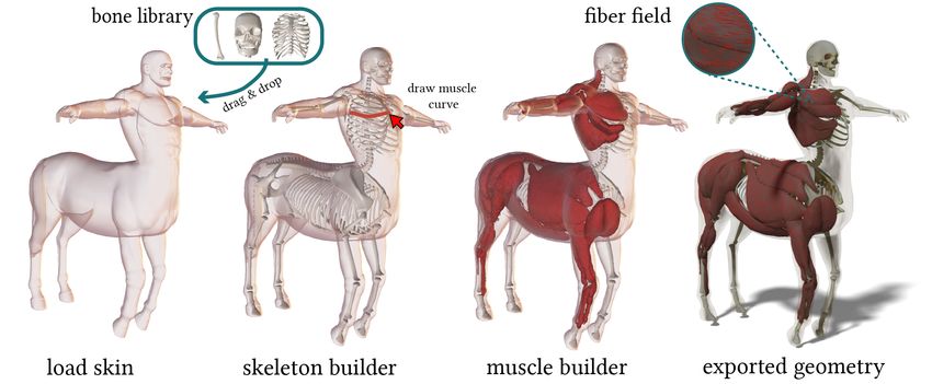
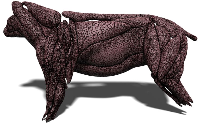
Interactive Modelling of Volumetric Musculoskeletal Anatomy
 RINAT ABDRASHITOV, University of Toronto, Canada
 SEUNGBAE BANG, University of Toronto, Canada
 DAVID LEVIN, University of Toronto, Canada
 KARAN SINGH, University of Toronto, Canada
 ALEC JACOBSON, University of Toronto, Canada
arXiv:2106.05161v1 [cs.GR] 9 Jun 2021

 Fig. 1. Given a skin surface mesh, a library of bone parts is used to quickly create a skeleton in our skeleton builder tool. The user then draws curves to generate
 the muscle shapes which are visualized using a volume rendering. Once all muscles are created, we can export the geometry of the muscles, automatically
 compute fiber fields and use the result in downstream applications. Centaur model is part of the TOSCA dataset [?]. Horse bone models were obtained from
 https://3dassets.store/. Used under permission.

 We present a new approach for modelling musculoskeletal anatomy. Unlike computation of muscle fiber fields. We further introduce a novel algorithm
 previous methods, we do not model individual muscle shapes as geometric for converting the volumetric muscle representation into tetrahedral or
 primitives (polygonal meshes, NURBS etc.). Instead, we adopt a volumetric surface geometry for use in downstream tasks. Additionally, we introduce
 segmentation approach where every point in our volume is assigned to a an interactive skeleton authoring tool that allows the users to create skeletal
 muscle, fat, or bone tissue. We provide an interactive modelling tool where anatomy starting from only a skin mesh using a library of bone parts.
 the user controls the segmentation via muscle curves and we visualize the
 CCS Concepts: • Computing methodologies → Mesh geometry mod-
 muscle shapes using volumetric rendering. Muscle curves enable intuitive
 els; Volumetric models; Graphics systems and interfaces.
 yet powerful control over the muscle shapes. This representation allows
 us to automatically handle intersections between different tissues (muscle- Additional Key Words and Phrases: anatomy modelling, 3D interface, diffu-
 muscle, muscle-bone, and muscle-skin) during the modelling and automates sion curves
 Authors’ addresses: Rinat Abdrashitov, University of Toronto, Toronto, Canada, rinat@ ACM Reference Format:
 dgp.toronto.edu; Seungbae Bang, University of Toronto, Toronto, Canada, seungbae@ Rinat Abdrashitov, Seungbae Bang, David Levin, Karan Singh, and Alec Ja-
 cs.toronto.edu; David Levin, University of Toronto, Canada, diwlevin@cs.toronto.edu;
 Karan Singh, University of Toronto, Toronto, Canada, karan@dgp.toronto.edu; Alec
 cobson. 2021. Interactive Modelling of Volumetric Musculoskeletal Anatomy.
 Jacobson, University of Toronto, Toronto, Canada, jacobson@cs.toronto.edu. ACM Trans. Graph. 40, 4, Article 122 (August 2021), 13 pages. https://doi.org/
 10.1145/3450626.3459769
 Permission to make digital or hard copies of all or part of this work for personal or
 classroom use is granted without fee provided that copies are not made or distributed
 for profit or commercial advantage and that copies bear this notice and the full citation 1 INTRODUCTION
 on the first page. Copyrights for components of this work owned by others than ACM
 must be honored. Abstracting with credit is permitted. To copy otherwise, or republish, Digital characters are a driving force in the entertainment industry
 to post on servers or to redistribute to lists, requires prior specific permission and/or a allowing artists to tell stories limited only by their imagination. A
 fee. Request permissions from permissions@acm.org. lot of effort goes into reaching a point where digital characters are
 © 2021 Association for Computing Machinery.
 0730-0301/2021/8-ART122 $15.00 indistinguishable from the real ones. Characters are often modeled
 https://doi.org/10.1145/3450626.3459769 by only considering their skin [Jacobson et al. 2014], disregarding

 ACM Trans. Graph., Vol. 40, No. 4, Article 122. Publication date: August 2021.

122:2 • Rinat Abdrashitov, Seungbae Bang, David Levin, Karan Singh, and Alec Jacobson

underlying volumetric muscle, fat, and bone structure. Animating
physically realistic effects like muscle bulging, skin sliding, wrinkles,
and volume preservation, without an explicit musculoskeletal struc-
ture is challenging and, and requires skilled and tedious manual
effort, to achieve high quality results. Therefore, a truly accurate
portrayal of digital characters requires the creation of biologically
representative musculoskeletal anatomy.
 Different solutions that allow artists to automate tedious manual
tasks like the creation of the skin [Yoshiyasu et al. 2014], hair [Saito
et al. 2018], rigs [Xu et al. 2020] and others have been explored
over the years. However, user-friendly solutions to the problem of
creating a musculoskeletal structure that is suitable for character
modelling and animation are relatively unexplored. The current so-
lutions either require artists to model every muscle using sculpting Fig. 2. Muscle structure. Image courtesy of [Lee et al. 2010]
software, go through tedious parameter tweaking of geometric prim-
itives, or create a detailed template for retargeting to new geometries.
These methods make it hard to produce complex intersection-free as "muscles". Internally, the muscle is composed of numerous mus-
muscle shapes that conform to the skin surface. Additionally, defin- cle fiber bundles, called fascicles. Large muscles, such as the biceps
ing muscle fiber directions requires users to manually specify at- brachii or the sartorius have fascicles arranged parallel to one an-
tachment points for every muscle. Making incremental changes other along the length of the muscle. Other muscles exhibit fascicles
using these approaches is tedious and hinders the fast exploration with a pennation angle, between their tendinous attachments and
of character design. the longitudinal axis of the muscle (Fig 2 bottom). Skeletal muscle
 We propose an interactive modelling tool, that adopts the out- is anchored by tendons to bone. Tendons transmit forces produced
side–in [Pratscher et al. 2005] approach and enables the creation of by the attached muscle to the bone, enabling locomotion and main-
a musculoskeletal system starting from a skin mesh. The user starts taining posture (Fig. 2 top). We refer the reader to the survey by Lee
by arranging the skeleton from pre-existing templates of bones. et al. [2010] which provides a thorough overview of modelling and
Then the user simply sketches curves inside a volume constrained simulation of skeletal muscles.
by the skin and our system automatically infers the muscle shapes.
Inspired by Orzan et al. [2008], we utilize a diffusion process to 2.2 Surface-based muscle primitives:
segment the volume into muscle and fat tissues based on the user- Musculoskeletal primitives for geometric character skinning is at
created curve network. The resulting muscles are intersection free least three decades old [Chadwick et al. 1989]. Early research has
and conform to the skin geometry. We show how to utilize volume explored the formulation of muscles as collections of ellipsoids
rendering to visualize the muscle shapes and hence avoid the need [Pratscher et al. 2005; Scheepers et al. 1997; Singh et al. 1995], gen-
for explicit meshing every time the user edits a curve. We further eralized cylinders [Simmons et al. 2002; Wilhelms and Van Gelder
propose an algorithm for extracting the manifold muscle meshes 1997], polygon meshes [Albrecht et al. 2003], extruded parametric
from our volumetric segmentation for the use in downstream tasks. curves [Tsang et al. 2005], NURBS [Autodesk 2021], and implicit
To the best of our knowledge, our system is the first user-friendly models [Roussellet et al. 2018]. These surface-based muscle primi-
interactive modelling tool, capable of creating intersection free tives typically serve as proxy geometry to bind and geometrically
geometry for the musculoskeletal system. deform a geometric skin. While these primitives can be imbued with
 simplified muscle dynamics, they are ill-suited to general purpose
2 BACKGROUND AND RELATED WORK anatomic simulation [Ziva Dynamics 2021]. Our representation,
 based on muscle curves and anisotropically induced muscle vol-
We provide a brief background on muscle anatomy followed by umes, provides the high-level geometric control of muscle shape
review of related work categorized by muscle representations in and skin deformation of these surface-based primitives, but can
physically-based animation; skinning methods that geometrically also produce various muscle shapes (parallel, convergent, pennate)
attempt to “emulate” the physics of muscle deformation; anatomic and automate the computation of fiber fields. Being an inherently
templates to aid character modelling, setup and transfer; and inter- volume-based representation, it is also well-suited to handle general
active interfaces for volumetric and character modelling. muscle-muscle, muscle-bone, muscle-skin intersections and muscle
 fiber bundle computations.
2.1 Musculoskeletal Anatomy:
Muscle is a soft tissue (of type skeletal, cardiac or smooth), whose 2.3 Volume-based muscle primitives:
function is to produce force and motion. A large body of research Physically-based simulation of the skin layered over volumetric
in Computer Graphics, biomechanics and robotics is focused on muscle primitives [Li et al. 2013] is a desirable solution to pro-
studying the physiological properties and and function of skeletal ducing the subtle details of skin motion [Weta Digital 2021; Ziva
muscles [Ng-Thow-Hing and Fiume 1997; Scheepers et al. 1997]. Dynamics 2021]. The initial musuloskeletal setup of a character as
For the rest of the paper, we will refer to "skeletal muscles" simply comprised of skin, fat, muscle and bone, in a simulation pipeline

ACM Trans. Graph., Vol. 40, No. 4, Article 122. Publication date: August 2021.

Interactive Modelling of Volumetric Musculoskeletal Anatomy • 122:3

is tedious and requires multiple iterations of laboriously rebuild-
ing hand-crafted bone and muscle geometry [Deepak Rajan 2021],
to elicit the desired simulation behavior from the musculoskeletal
anatomy. These sculpted geometries then need to be processed to
resolve intersections, and define fiber fields to support anisotropic
muscle contraction. While MRI/CT scan data can aid the recon-
struction of accurate live anatomy [Jacobs et al. 2016; Teran et al.
2005], such data must be artist-imagined for fictional characters.
Muscles have also been built by physically simulating inflatable
3D patches defined by a user on a character’s skin [Turchet et al.
2017], or as parametric solid volumes [Ng-Thow-Hing and Fiume Fig. 3. The skeleton and muscle builder UIs.
1997], but these muscles tend to leave undesirable gaps between
muscles, bones and other internal structures. Angles et al. [2019]
models a muscle as a bundle of position-based rods augmented with
 the “building-blocks” of an object, such as SDF instances and region
isotropic scale to enable simulation of volumetric effects. However,
 definitions, and then assemble them together into linked SDF trees.
their rod-based representation requires users to either manually cre-
 Several sketch-based interfaces for character modelling [De Paoli
ate bundles or acquire pre-existing tetrahedral geometry of muscles
 and Singh 2015; Nealen et al. 2007; Schmid et al. 2011; Takayama
which is then automatically converted to their representation. Yu
 et al. 2013] use a 3D geometric skin as a canvas on and around
et al. [2020] introduces an efficient algorithm for (self)-repulsion of
 which to project 2D sketch strokes. Our work is similar in spirit
space curves that can be used to design biologically-inspired curve
 to [De Paoli and Singh 2015; Schmid et al. 2011] in that we are
networks such as muscle fibers. However, their optimization-based
 focused on drawing curves, around the skin, and specifically within
approach is not suitable for interactive modelling of a large number
 a volumetric domain constrained by the surface of the skin.
of muscles.
 The actual shape of the muscles is inferred from the scalar values
 defined on the curves via a volumetric rendering approach. We do
2.4 Anatomic Templates: not explicitly generate the geometry (triangle or tetrahedral meshes)
The first semi-automatic method for creating anatomical structures, of the muscles until the user completes the modelling session. Unlike
such as bones, muscles, viscera, and fat tissues was proposed by previous methods, our approach allows the user to rapidly explore
Ali-Hamadi et al. [2013]. Their method can be seen as a partial and experiment with both the topological connectivity and shape
registration process, where skin surfaces are first registered based of musculoskeletal structures, with a guarantee of precisely con-
on the data, and the interior tissues are estimated using interpola- strained and intersection-free structures that conform outside-in to
tion and anatomical rules. Saito et al. [2015] create a wide range of the given skin surface.
human body shapes from a single input 3D anatomy template by
simulating biological processes responsible for human body growth. 3 OUR SYSTEM
Kadleček et al. [2016] use a set of 3D scans of an actor in various The user starts by providing the skin mesh of a model. The bone
poses to compute subject-specific and pose-dependent parameters meshes can also either be provided by the user or built using our in-
of an anatomical template model, to explain the captured 3D scans terface (Fig.3 left). We generate the tetrahedral mesh T ∈ R |T|×4, V ∈
as closely as possible. Our method is complementary to these ap- R |V |×3 from combined skin and bone geometries to make sure our
proaches and can be used to produce the initial template. tetrahedralization conforms to the bone geometry. We remove
 all tetrahedra belonging to the bone geometry. This simultane-
2.5 Interactive volumetric and character modelling: ously induces desirable natural boundary conditions (see, e.g., [Stein
Takayama et al. [2010] proposed a novel diffusion surface (DS) rep- et al. 2018]) and increases computational performance. A tablet or
resentation to model the smooth color variation seen in fruit and a mouse can be used to draw an open 2D stroke that starts and
vegetables. User input to their approach, and others [Owada et al. ends over the bone surface. The muscle surface corresponding to
2008; Pietroni et al. 2007] is based on cross-sections, which are ill- the drawn curve is presented to the user. The user can continue to
suited to modelling complex muscle geometry and connectivity. draw more strokes or edit the existing ones to create a full muscular
Solid texture synthesis [Pietroni et al. 2010] is focused on modelling system (Fig.3 right). The results can then be exported as surface
homogeneous material like wood or marble and Cutler et al. [2002] or tetrahedral meshes and further edited in other software pack-
uses scripting to define internal volumetric structure of mesh(es). ages. In the following sections, we describe each part of our muscle
Yuan et al. [2012] do facilitate solid modelling of heterogeneous modelling system and discrete implementation in detail.
objects with multiple internal regions using multiphase implicit
functions. However, these approaches are not artist-centric or re- 3.1 Skeleton Authoring
quire segmented and labeled 3D biomedical images as input. Wang If pre-existing skeletal geometry is not available, we provide a tool
et al. [2011] represent complex internal 3D structure using multi- for creation of the skeletal system from the pre-existing library of
scale vector volumes. The object is decomposed into components bones. We define a three categories for the types for bones: cylinder
modelled as SDF trees. However, the user needs to actually create bone, curve bone, shape bone. The user can select a pre-defined

 ACM Trans. Graph., Vol. 40, No. 4, Article 122. Publication date: August 2021.

122:4 • Rinat Abdrashitov, Seungbae Bang, David Levin, Karan Singh, and Alec Jacobson

templates for each of the categories. Then each of template bones are
properly placed inside the body mesh with the algorithm described
below.

3.1.1 Cylinder bone. A cylinder bone is a type of bone that can
be represented as a line segment (e.g. arm or leg bone). When a
user clicks on a point on the surface of the skin mesh, we cast a ray
through the mesh and record the first two hits, which correspond
to the ray entering and exiting the mesh, respectively. We take the
midpoint of these two intersections as one endpoint of the cylinder
bone, and the other endpoint is determined interactively using the Fig. 4. three types of bone in our skeleton authoring interface, and pre-
same ray-casting procedure while the mouse button is held down. A rigged on cage deformer of shape templates.
cylinder bone template is pre-rigged with two point handles and it
is deformed accordingly as its two point handles are attached with
the endpoints of the line the user draw. The depth value for all the points drawn in be-
 tween is ambiguous, so we simply linearly in-
3.1.2 Curve bone. Curve bone is a type of bone that can be rep- terpolate the depths of the first and last points.
resented as a curve. For example, a spine can be described as a Because we want the curves to be easily ed-
sequence of vertebrae bones placed along a curve. When the user itable we fit a Catmull–Rom spline S in a
draws a curve, it is projected onto a user-defined plane of symmetry. least squares manner with 4 control points
Then for easy editing of the curve, we fit a Catmull-Rom spline to a 1, ..., 4 by default: one for each end point
given points on plane. Finally, a user selected template is distributed and two along the curve (see inset). We de-
along the spline. note the resulting muscle curve network as
 a set of splines {S1, S2, ..., S }. Each control
3.1.3 Shape bone. A shape bone is a type that cannot be repre- 
 point is augmented with an additional at-
sented as a line segment nor a curve. Essentially, it describes all 
 tribute representing a tissue value . Users can adjust the tissue
the bones with complex shapes. We place the shape bone as local
 value to shape the muscle: a larger value results in a "thicker" shape
fitting on the user-specified region. We determine the center of the
 around the control point.
template with a mouse click, using the same raycasting procedure
used to compute the endpoints of a cylinder bone. Then from that
 3.3 Muscle and Fat Functions
initial shape, the template is iteratively fitted to its local region of
the skin mesh. Let Ω ∈ R3 denote the volumetric domain defined by the tetrahedral
 mesh V, T. Our goal is to find a scalar muscle function : Ω → R
3.1.4 Local fitting. We pre-rigged the template with a cage de- for each muscle that describes the likelihood of any point ∈ Ω
former. Using data that already has skin and corresponding bone to belong to a muscle . Similarly we define a fat function that
mesh, we define a cage by cutting a local region of the skin mesh describes the likelihood of any point to belong to a fat layer. We
with high decimation and with manual editing. We fit the cage propose to define and as minimizers of the Dirichlet energy
using both step of rigid ICP (Iterative Closest Point) and nonrigid subject to constraints:
ICP, and the templates are deformed using this registered cage. We ∫
 ∑︁ ∫
first perform rigid ICP to find an optimal transformation of its clos- argmin ∇ A ∇ + ||∇ || 2 (1)
est corresponding target points. After it has converged within the , , =1,..., =1 Ω Ω
threshold, we then perform nonrigid ICP by deforming the cage subject to | Ω = (2)
with an additional squared Laplacian smoothness term to prevent | Ω =0 ∈ {1, ..., }, ≠ (3)
abrupt deformation. Corresponding target points are determined by
 | Ω=0 (4)
finding the closest points to cage vertices on the skin mesh. We dis-
card the correspondence point whose normal directions are almost | Ω= fat (5)
opposite to their closest projected points | Ω =0 ∈ {1, ..., } (6)
 where A is an optional user-defined diffusion tensor field which
3.2 Muscle Curve Authoring biases the directions in which material flows at a point in space.
The user draws a curve for each muscle. Skeletal muscles require Intuitively, we "diffuse" each muscle curve such that the tissue values
an origin and insertion points where the muscle tendons are be- at the curve points ( Ω ) are set by the user (via interpolation of
ing attached to the bone. In our interface we expect the user to 
 tissue values at the control points) and the tissue values at
always begin and end the stroke over the bone surface and provide all other muscle curves ( Ω ) and skin ( Ω) are set to zero. We
the necessary visual feedback to achieve that. The first and last additionally diffuse from the skin to represent the fat layer (fat
points of the curve are automatically projected via ray-casting onto function , where "s" stands for skin) by setting its tissue value to a
the surface of the bone to find their corresponding 3d coordinates. user-defined fat and constraining the values at all muscle curves

ACM Trans. Graph., Vol. 40, No. 4, Article 122. Publication date: August 2021.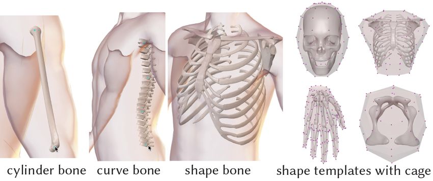

Interactive Modelling of Volumetric Musculoskeletal Anatomy • 122:5

 constraint equation:
  B1   d1 
    
 B f =  .  f =  ..  = d ∈ R |C |
  ..   . 
 (8)
    
 B  d 
    
 where for every curve = {1, ..., } we have B ∈ R |C |×|V | which
Fig. 5. 2D example of two muscle curves in red and skin layer in aquamarine is a sparse matrix of stacked barycentric coordinates of collocation
(a). User defined tissue values at each curve ( Ω1 , Ω2 ) are diffused (b,c)
 points for all curves with non-zero entry B ( , ) being a barycentric
to compute corresponding muscle functions ( 1 , 2 ). Additionally fat tissue
values defined at skin vertices are diffused to compute the fat function 
 coordinate of the collocation point with respect to vertex , d ∈
(d). R |C | is a vector of stacked tissue values of collocation points s.t.
 d ( ) is nonzero only if collocation point belongs to curve and
 f ∈ |V | are values of muscle function at each vertex of the
 tetrahedral mesh. The fat tissue constraint (Eq. 6) can be similarly
to be zero (Fig. 5). The fat function always diffuses isotropically discretized as
and hence is written as a separate term. The vertices that belong to  B1 
  
the bone surface do not “diffuse” bone tissue material but instead B f =  ..  f = 0 ∈ R |C |
  . 
 (9)
participate in the optimization as natural (zero normal derivative)  
 B 
boundary conditions.  
 The Dirchlet Energy in Eq.1 is discretized as
3.4 Discretization 
 ∑︁
 min (f L̃ f + ||B f − d || 2 ) + f L f + ||B f || 2 (10)
The muscle splines usually do not coincide with the vertices of the
 =1
tetrahedral mesh and to discretize the splines we need to identify
 subject to f | = 0 (11)
a set of tetrahedrons that contain each muscle curve Si . For each
tetrahedron and each muscle curve passing through it, we identify f | = dfat (12)
a point c ∈ R3 on the curve that is contained inside the tetrahedron 
 L̃ = G M̃A G (13)
(see inset).
 In practice, we choose the point to where G is the gradient matrix (see [Botsch et al. 2010] for deriva-
be the midpoint of the curve segment tion) and M̃ is a mass matrix representing an inner-product account-
bounded by the tetrahedron. We call ing for the volume associated with each tetrahedron, G M̃AG is the
this point a collocation point. All collo- anisotropic cotangent Laplacian ([Andreux et al. 2014]), L is the
cation points can be found efficiently by standard (isotropic) cotangent Laplacian, parameter that defines
finding the tetrahedron containing the the tradeoff between smoothness of the resulting scalar field and
first curve point and then finding all the respecting the tissue values at the collocation points (set to 5 in
other tetrahedrons by tracing the curve, given that the adjacency is our experiments). Because the collocation points are not necessarily
computed beforehand. This amounts to at most three ray triangles located at mesh vertices and many may appear in the same element,
intersections per tetrahedron and therefore very fast. using soft constraints avoids overshooting. Vertex values f of each
 For each curve , we stack all collocation points in a matrix C ∈ muscle function can be computed separately and hence computa-
R |C |×3 and compute a tissue value for each collocation point tion of Eq.10 is easily parallelizable. Compared to regular-grid-based
 methods, the boundary-conforming tetrahedral mesh makes it easy
by interpolating values at control points . One of the primary
 to set precise boundary conditions.
constraints to be satisfied (Eq. 2, 3) are the curve constraints, i.e.,the
tissue value at the vertices V must be determined to agree with the
 3.5 Segmentation
values at the collocation points. We use barycentric coordinates
to interpolate the tissue values for each tetrahedron, such that the Each point ∈ Ω in our volume will either belong to a muscle, bone,
value of the collocation point is expressed as: or fat. The fat is visually represented as an "empty" space between
 muscles, skin, and bones. The points that belong to the bone tissue
 4
 are simply all the points that are contained inside tetrahedrons
 comprising the bone geometry. So we only need to differentiate
 ∑︁
 = ∗ (7)
 =1 between muscles and fat. We treat the muscle and fat functions as
 probabilities and assign the point to the tissue with the highest
where denotes the tissue value of a vertex of a tetrahedron probability (Fig. 6):
(for = 1, 2, 3, 4) to which the collocation point belongs to, and ( ) = argmax ({ 1 ( ), ... ( ), ( )}) (14)
 are the barycentric coordinates of with respect to the vertex 
 . Stacking the barycentric equation (7) for a set of desired values In the discrete case we find the tetrahedron that contains the point
of the collocation points into a matrix constitutes a linear equality and use barycentric interpolation to determine tissue values for

 ACM Trans. Graph., Vol. 40, No. 4, Article 122. Publication date: August 2021.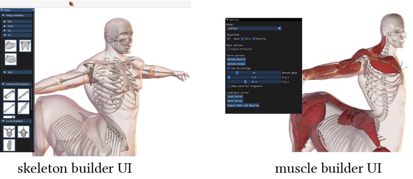

122:6 • Rinat Abdrashitov, Seungbae Bang, David Levin, Karan Singh, and Alec Jacobson

Fig. 6. Each point in our domain has a vector of tissue values that represent
the likelihood of this point to belong to one of the tissues (left). We assign
the point to the tissue with the highest probability (right).

muscles and fat at given tissue values (f1 ..f 
 , f ) at the vertices of
 
the tetrahedron . We skip the normalization step of our probabilities
because the muscle visualization (Sec 3.6) and muscle extraction
(Sec 4) are invariant to normalization.

3.6 Visualization
In the end, we only want to visualize all points belonging to the mus-
cles, while points belonging to fat should be invisible. A common
solution to this problem in scientific visualization and computer
graphics is volume rendering. We take inspiration from the litera-
ture on volume rendering on unstructured grids ([Silva et al. 2005;
Weiler et al. 2003]) which deals with rendering isosurfaces of a scalar
function defined on vertices of the tetrahedral mesh. To achieve in-
teractive rates we perform ray casting on the graphics hardware via
a ray propagation approach and perform all computation inside a
fragment shader.
 To render the model we split each tetrahedron into 4 triangles and Fig. 7. The user has additional control over the muscle shape by changing
submit them for rendering on the GPU. For each vertex of the trian- the rate of diffusion along the certain directions.
gle, we assign a vertex attribute with the value of the tetrahedron
index it belongs to and set it to not be interpolated when moving of the tetrahedron (see inset). A face is visible if the denominator in
from vertex to fragment shader. That way each fragment can be the previous equation is negative; thus, this test comes almost for
traced back to the tetrahedron it belongs to. We store all the infor- free. If is set to an appropriately large number for all visible faces,
mation (vertex positions, normals, muscle and fat functions) about min{ |0 ≤ < 4} identifies the exit point. Once the minimum 
each tetrahedron on the GPU and access it inside the shader. and its face are identified, the intersection point may be computed
 Inside the fragment shader, we start with as = + .
computing the entry point into the tetrahedron The muscle surface is only potentially visible if the entry point
that the current fragment belongs to by simply belongs to fat in which case we ray march through the single
converting the fragment from screen space into tetrahedron from the entry point to the exit point until we de-
camera space. We determine the correspond- tect that the tissue changed from fat to muscle. At which point we
ing exit point by computing three intersection stop and compute the normal to shade the surface of the muscle.
points of the ray with the planes containing If the whole tetrahedron belongs to fat we call the GLSL discard
faces of the entered tetrahedron and choosing command and the GPU will call the shader again until we find a
the intersection point that is closest to the eye tetrahedron that contains the surface of a muscle (if one exists).
point but not on a face that is visible from the Figures 1, 7 show an example of a volume-rendered muscles.
eyepoint. With the eye point , and the normal-
ized direction of the viewing ray, the intersection points with the 3.7 Anisotropy
faces of the tetrahedron are + with 0 ≤ < 4: To provide an additional control over the muscle shape we allow
 ( 3− − ) · users to change the rate of diffusion along the certain directions. This
 = (15)
 · is achieved by introducing a tensor field that biases the directions in
where ∈ {0, 1, 2, 3} denote the face index, is the vertex opposite which tissues diffuse at a point in space. Tensor field is represented
to the -th face, is the normal vector of the face pointing outside by a tensor matrix A ∈ R |G |×|G| in Eq. 13.

ACM Trans. Graph., Vol. 40, No. 4, Article 122. Publication date: August 2021.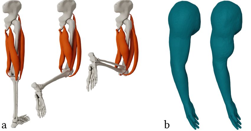

Interactive Modelling of Volumetric Musculoskeletal Anatomy • 122:7

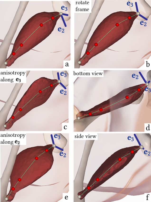
 We provide an easy way for the user to construct the tensor whose domain of definition is a -simplex, namely the orthogonal
fields for the individual muscles. The first point of each muscle projection of , onto the hyperplane +1 = 0. The upper enve-
curve is assigned a 3D frame Q = [e1 e2 e3 ] ∈ R3×3 representing lope, , of the given simplices is the pointwise maximum of these
eigenvectors of a tensor. The first vector in the frame e1 is always functions [Edelsbrunner et al. 1989], that is,
aligned with the curve tangent while the other two eigenvectors
lie in its null space. The user has control over the rotation of e2, e3 ( 1, 2, ..., ) = max ( 1, 2, ..., ) (16)
 1≤ ≤ 
along the axis defined by e1 (Fig. 7ab). Additionally, the user can
control the magnitude of eigenvalues 2, 3 to bias diffusion rate The maximization diagram MS of is the subdivision of into
along e2, e3 directions (Fig. 7cdef). We use the method of [Hanson connected cells obtained by the projection of the upper envelope
and Ma 1995] to compute the frame Q at each collocation point of in the direction. The example in Fig. 9 corresponds to =
 , and assign frames to each vertex of the tetrahedrons containing 1 where each line segment is a 1D simplex in 2D space. Fig. 8a
collocation points (using the frame of the closest collocation point). shows an example of two 2-dimensional simplices in 3-dimensional
 Each frame Q can be considered as a set of nine scalars and space whose maximization diagram is shown in (Fig. 8b). Solutions
the problem of propagating values from the fixed vertices of the for solving the general upper envelope problem for = 1 and
tetrahedrons containing collocation points to the remaining vertices = 2 ([Agarwal et al. 1996; Meyerovitch 2006]) and computing
is thus same as computing nine scalar fields over the mesh. To find their corresponding maximization diagrams have been proposed.
the unknown values at the remaining vertices, we use the Laplacian Abdrashitov et al. [2019] computes = 2 upper envelope of "part"
smoothing framework, i.e. for each scalar field, we create a harmonic functions to extract the smoothed part boundaries.
vertex-based scalar field on T given the boundary conditions (from We consider tissue functions T = { 1, ..., , } (combination of
the values at the fixed vertices) [Palacios et al. 2016]. Once all 9 muscle and fat functions) defined as scalar fields over the vertices
scalar fields have been obtained, we compute the per-vertex tensor of our tetrahedral mesh and we notice that Equation 14 is the point-
Q ΛQ where Λ contains eigenvalues 1 2 3 along the diagonal and wise maximum (Eq.16) of tissue functions. In our problem ( = 3)
assemble the tensor field matrix A for the muscle . we are interested in finding maximization diagrams of all tissue
 functions over the volume constrained by the surface of the skin.
 This problem can be solved by considering finding the maximization
4 MUSCLE EXTRACTION diagrams of the tissue functions over each tetrahedron. In which
Given the complete muscle curve network and the corresponding case in contrast to the general upper envelope problem where our
muscle functions defined over the volumetric domain, we need domain is a continuous hyperplane, we restrict our domain by a
to extract the geometry of the muscles suitable for downstream 3-simplex on that hyperplane. Fig. 8c shows an example of the maxi-
applications. mization diagram of the functions defined by the scalar values at the
 Isosurface extraction methods [Chentanez et al. 2009; Labelle and vertices of the tetrahedron and (Fig.8d) shows the tetrahedralization
Shewchuk 2007; Lorensen and Cline 1987] do not trivially solve our of each cell. As a result, the tetrahedron is split into more sub-tets
problem, because we are not simply extracting an isosurface of a where each sub-tet has only one function that is the maximum.
scalar function. Instead, we want compute a pointwise maximum In other words, we can "assign" the sub-tet to one of the tissues.
of multiple scalar functions inside each tetrahedron and extract a Performing this operation for every single tetrahedron results in a
boundary separating each function while ensuring the final output is new tetrahedral mesh where each tetrahedron is assigned to one
a manifold tetrahedral mesh. In other words, inside each tetrahedron, tissue. We can extract individual tissue shapes by simply combining
each tissue function can be thought of as a point-wise vote for all tetrahedrons that are assigned to that tissue. Fig. 8e shows an
ownership. We want to split the tetrahedron along boundaries that example of taking a uniform 3x3 tetrahedral mesh with two scalar
delineate changes in the maximum vote and assign each sub-tet to functions defined over it and splitting it into two tetrahedral meshes
the tissue with maximum value. We cast the problem of extracting (Fig.8f). The split is the result of computing tetrahedralized max-
the muscle surface geometry as a solution to the computation of imization diagrams of every tetrahedron. However, the resulting
the upper envelope of scalar functions representing each tissue over tetrahedral meshes representing each muscle are not guaranted to
each tetrahedron. First, lets look at a simple example of the upper be manifold unless we are consistent with how we tessellate adja-
envelope problem in Fig. 9. Four line segments are defined over cent tetrahedrons (Fig. 10). In reality, we would just be getting a
the 1D domain [ , ] (Fig. 9, left). The upper envelope is the point- tetrahedral "soup" that is difficult to work with. Instead we want
wise maximum of all segments over the domain. The maximization our resulting mesh to be manifold and hence we can easily use it
diagram is a subdivision of the domain [ , ] into cells, where each for downstream applications. We propose an algorithm for comput-
cell’s identity is induced by the upper envelope. Alternatively, we ing manifold tetrahedralized maximization diagrams of functions
can think of the maximization diagram as a projection of the upper defined as scalar fields over the vertices of a tetrahedral mesh. We
envelope onto the domain (Fig. 9, right). first define auxiliary operations in Sections 4.1, 4.2 and then discuss
 Let us now define the general upper envelope problem. Let = the main algorithm in Sections 4.3.
{ 1, 2 ...., } be -simplices in ( + 1)-dimensional space. A -
simplex has ( + 1) vertices, i.e. = 1 is a line segment, = 2 is a 4.1 Prune tissues
triangle and = 3 is a tetrahedron. We can thus view each , as the We notice that if the tissue function ∈ T is strictly below any
graph of a partially defined linear function +1 = ( 1, 2, ..., ), other tissue function , then it will not be part of the maximization

 ACM Trans. Graph., Vol. 40, No. 4, Article 122. Publication date: August 2021.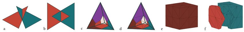

122:8 • Rinat Abdrashitov, Seungbae Bang, David Levin, Karan Singh, and Alec Jacobson

Fig. 8. Two triangles (a) and the corresponding maximization diagram (b). Example of the maximization diagram cells of 5 different functions over the
tetrahedron (c) and tetrahedralization of each cell (d). Tetrahedral mesh (e) with 2 different functions defined over its vertices and the resulting tetrahedralized
maximization diagram (one of the parts is slightly moved in the figure to show the internal tessellation)

 Fig. 11. Split the edge over

Fig. 9. Four line segments (red, green, purple, gray) are defined over a
single 1D element [ , ] (left). The upper envelope (light blue) and the along the isosurface and tetrahedralizing the resulting polyhedrons.
maximization diagram (right).
 Input: tetrahedron defined by 4 vertices V ∈ 4×3 , per-vertex val-
 ues f ∈ 4 of a scalar function .
 Output: tet mesh T ,V resulted from splitting the input tet
 along the isosurface of at isovalue of 0.

 Algorithm: We find a set of sorted unique edges E of the tetrahedron
 that are intersected by the isosurface of . The number of edges | |
 is either 3 or 4. We then define a split_edge operator that given a
 tetrahedron and an edge first splits the edge at a vertex and
 then splits into two tetrahedrons by connecting with two vertices
 of the edge opposite (Fig. 11). Similarly to Marching tetrahdera
 the location of is determined by interpoloating vertices of us-
 ing weights defined by . We simpy run split_edge recusively on
Fig. 10. Maximization diagram is defined over two adjacent tetrahedrons each ∈ E to produce the resulting tetrahedral mesh T . The
1234 and 1345 (a). During the tessellation there is no guarantee that the order of edges in E determines the order in which we split the edges
shared face 134 is split the same way (b). By making sure the order of edge and hence determines the final topology of the tessellation. By sim-
splits is consistent we can guarantee that the face is split the same way (c). ply sorting the interested unique edges we solve the problem of
 inconsistent tessellation (Fig.10b) between adjacent tetrahedrons
diagram and hence can be ignored and help avoid unnecessary (Fig.10c). We additionally maintain a history of unique edge splits
computations. We define the sparse matrix W ∈ {0, 1} +1× +1 before splitting an edge at vertex . If the edge was split before
where W = 1 if and only if there exist at least one tetrahedron in at vertex ˆ by a call to split_edge on one of the adjacent tetrahedron
T whose maximization diagram contains cells assigned to tissues we do not create a new vertex but simply make it point to . ˆ To
and . improve the robustness of the algorithm, when almost coincides
 with one of the vertices in V (when one of the values in f is close to
4.2 Split tetrahedron zero within some thereshold) we simply remove that edge from E
Given only two different tissue functions 1 and 2 over a tetrahedron so it will not be split.
we need to find the tetrahedralized maximization diagram that re-
sults from computing the upper envelope of those two functions. 4.3 Tetrahedralized Maximization Diagram
This problem is similar to the Marching tetrahedra [Doi and Koide We iterate through every tissue function ∈ T and use W to find
1991] algorithm that finds an isosurface of a scalar field 1 − 2 a set of tissue funtions T̂ such that for any ∈ T̂ , W( , ) > 0. In
passing through isovalue of 0. However, in our case we are not other words T̂ contains all tissue functions that appear in the maxi-
interested in extracting the isosurface but rather splitting the tet mization diagrams with in at least one tetrahedron. We compute

ACM Trans. Graph., Vol. 40, No. 4, Article 122. Publication date: August 2021.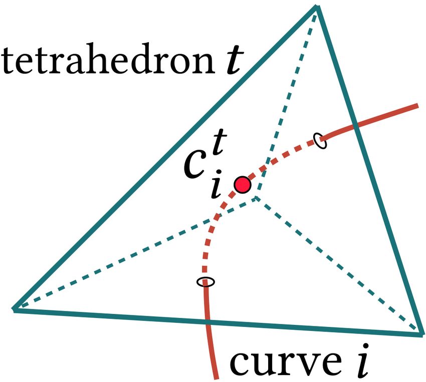

Interactive Modelling of Volumetric Musculoskeletal Anatomy • 122:9

all pairs { , } of the tissue with tissues in the set T̂ . For every
pair we iterate through all tetrahedrons ∈ T with corresponding
4 vertices V and call the SplitTet subroutine. Algorithm 1 summa-
rizes our divide and conquer approach to computing tetrahedralized
maximimzation diagram of tissue functions T̂ over the tetrahedral
mesh T, V.

 Algorithm 1: Tetrahedralized Maximization Diagram
 Input: Tet mesh T, V and per-vertex tissue values
 X ∈ R |V |×( +1) Fig. 12. Parallel, Fusiform, Triangular, Unipennate.
 Output: Tet mesh T , V and per-tet tissue labeling L 
 W = PruneTissues( ); # Section 4.1 for each tissue do
 T̂ =FindIntersectingTissues( , W) for every pair vertices within a threshold distance of the
 ( , ) ∈ T̂ do curve endpoints. This term forces the gradi-
 for ← 1 to |T| do ent of the scalar field in T to align with
 V ,T = SplitTet(V , X( , ) − X( , )); the curve’s tangent vector. The inset figure
 //using barycentric interpolation to compute all shows an example of a tetrahedron that inter-
 tissues values for all ∈ V sects the muscle curve where gradient g of the scalar field is aligned
 X = InterpolateDiffusion(V , T, V, X); with the tangent vector t via constraining g to be orthogonal to the
 //replace with first tetrahedron in T , append null space of t which is represented by n̂1 and n̂2 . The fiber field can
 the rest then be computed as the normalized gradient of u, i.e., ∇u/||∇u||.
 UpdateT(T, T );
 V = [V; V ]; 5 IMPLEMENTATION AND RESULTS
 X = [X; X ]; Skeletal and muscle curve authoring tools are implemented as sep-
 end arate standalone C++ applications using Eigen [Guennebaud et al.
 end 2010], libigl [Jacobson et al. 2013], and, for the user interface, ImGui.
 end The output of the skeletal authoring tool are skin and bone triangu-
 lar meshes. We exploit the fact that due to symmetry one only needs
 to use half of the mesh for creating the muscles. Therefore, we cut
 both skin and bone meshes along the half-plane. The mesh vertices
4.4 Fiber direction belonging to the cut boundary can be excluded from the constraints
Fiber directions play an important role in simulation by defining in Eq. 11, 12 to help create muscles that are suppose to cross the cut
the directions the muscle contracts. Fibers tend to point in the same boundary. The half-skin and half-bone meshes are loaded by the
directions as gradients of a hypothetical flow from one end of the muscle-curve authoring tool and we use TetGen [Si 2015] to gener-
muscle to the other [Choi and Blemker 2013; Saito et al. 2015]. Given ate a tetrahedral mesh. The quadratic solver is implemented using
muscles tetrahedral mesh V , T , we leverage our muscle curve to the modified version of libIGL’s min_quad_with_fixed function with
guide the global flow of the fiber field. The flow should align with Eigen’s PardisoSupport module which provides significant speed
the tangent space of the muscle curve. This can be formulated via ups. The tool was tested on a computer with Intel Xeon CPU @
constraint that for each tetrahedron along the curve we would like 2.40GHZ, Nvidia GTX1080 and 64GB of RAM and can perform at
the projection of the gradient onto the normal space to be zero. interactive rates for tetrahedral meshes with > 500k tetrahedrons.
 Let T ∈ T be a subset of tetrahedrons that the muscle curve The geometry stays intact between curve editing operations, and
intersects. Then the desired "flow" can be found by solving the we only update GPU buffers containing per-vertex diffusion values
energy minimization problem: which is fast.
 Figure 16 showcases the results created by the authors using our
 min u L u + (NGu) (NGu) (17) tool. We informally evaluated our tool with a professional anima-
 subject to u = 0 (18) tor who has experience with using Maya Muscles [Autodesk 2021]
 u = 1 (19) for creating musculoskeletal systems. They mentioned that using
 existing tools requires a significant amount of tedious work for
 u 
 =0 (20) ensuring that muscle geometry respects the geometry of its sur-
 n̂ roundings (bones, skin, other muscles), and the overall workflow
 where G ∈ 3|T |× |V | is a gradient ma- is "unintuitive" and "awkward". They liked the fact that our tool
trix, N ∈ R2|T |×3|T | is sparse matrix allows one to simply draw the location of the muscle while handling
containing 2 vectors per gradient vector rep- these issues automatically and provides enough intuitive controls
resenting the null space of the curves tan- (changing tissue values, moving control points, enabling anisotropy)
gent vector, u and u are a subset of to create complex muscle shape (Fig.12). One feature they wanted

 ACM Trans. Graph., Vol. 40, No. 4, Article 122. Publication date: August 2021.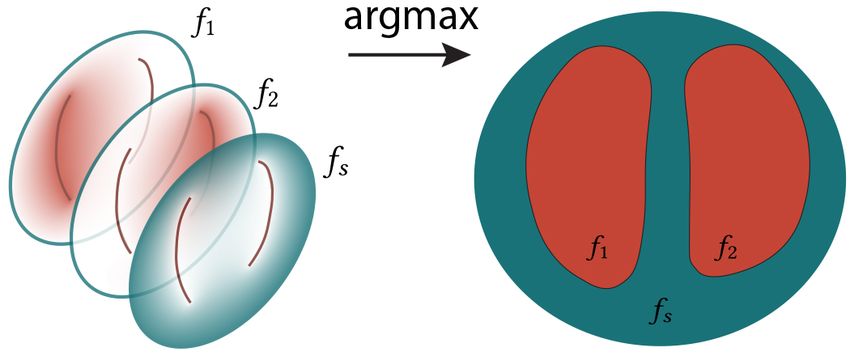

122:10 • Rinat Abdrashitov, Seungbae Bang, David Levin, Karan Singh, and Alec Jacobson

Fig. 13. We consider the Lion model in Fig. 16 with 39 muscles and 642224
tetrahedrons. The plot shows the number of tetrahedrons and the maximum Fig. 14. Example of the final tessellation produced by the upper envelope
number of tissue functions that can appear in their corresponding maximiza- algorithm.
tion diagram. This shows that for the vast majority of tetrahedrons (78%)
computing their tetrahedralized maximization diagrams requires no split-
ting or only trivial non-recursive splitting of 2 tissues (19%). No tetrahedrons
require resolving intersection of 6 or more tissues.

to see added is volume preservation of the muscle: when a muscle is
being flattened in one direction, there is a corresponding stretching
in another direction so that the volume stays the same. They also
wanted an ability to specify multiple attachment points instead of
just two to enable finer control, especially for triangular types of
muscle shapes. We further informally evaluated our tool with an
orthopedic surgeon with extensive knowledge of human anatomy
but who does not have experience with 3D modelling applications.
They see the potential of using this tool to explain the surgery pro- Fig. 15. Simulating the motion of a leg using muscle geometry created
cess to their patients. By using a pre-existing anatomical muscle with our tool without contact handling. Motion is induced by contracting
model made with our tool, they would be able to edit the muscles to the hamstring using the method of Modi et al. [2020] (a). Dynamic Finite
explain their medical procedure. However, similar to the animator, Element simulation of isometric contraction of the bicep using linear tetra-
they mentioned that to create truly anatomically correct muscles, hedral finite elements. Muscles are modeled as Neohookean elastic solids
they need to be able to specify multiple attachment points. using the fiber model of Teran et al. [2003]. Time integration is performed
 The muscle extraction algorithm in Section 4 uses the divide and via Implicit Euler time stepping using the Bartels library [Levin 2020]. We
 refer the reader to the provided Additional Modelling and Simulation De-
conquer approach by considering pairs of tissue functions. In Figure
 mos (07:30m) video to see the animated examples. Bone geometry (left) is
13, using the example of the Lion model (Fig.16), we show that provided by ©Ziva Dynamics. Used under permission.
in practice the vast majority of tetrahedrons only contain 1 tissue
function in their maximization diagram and therefore are not split.
While the vast majority of tetrahedrons that do need to be split only values of the tissue functions (Eq. 10) for each vertex of the tetra-
contain 2 tissue functions, which means they are only split once. hedral mesh and update those values in the corresponding GPU
 Because our volumetric domain is represented as an unstructured buffer. These values are later accessed by the fragment shader to
mesh, the resulting topology of the muscle meshes ends up contain- perform the volumetric rendering using the ray-marching method
ing skinny tetrahedrons as shown in Figure 14. However, because (supported by all modern GPUs). The muscle visualization using
we guarantee that the resulting meshes are manifold, it is straight- fragment shaders is fast (>30fps) on our system. The bottleneck of
forward to extract the boundary faces (faces that belong to only one our system during modeling is computing the solution to (Eq. 10) for
tetrahedron). The resulting muscle surface triangular meshes can which we currently use the Eigen library with Pardiso enabled. This
be easily remeshed and tetrahedralized again. In practice, we simply solve immediately benefits from any generic Poisson solving opti-
run TetWild [Hu et al. 2018] with default parameters on the surface mizations which are orthogonal to our main contributions. We only
mesh to improve the topology. perform a meshing operation (Sec. 4) after the modelling session is
 During the modelling process the muscles seen by the user are di- complete, to export muscles as tetrahedral meshes for downstream
rectly volume rendered upper-envelopes: rendering does not require applications. Using muscle extraction every time we create/edit a
performing any meshing operations during the modeling process. muscle would negatively impact performance, which is the motiva-
Every time the user creates or edits muscle curves we recompute tion for our volumetric rendering approach.

ACM Trans. Graph., Vol. 40, No. 4, Article 122. Publication date: August 2021.

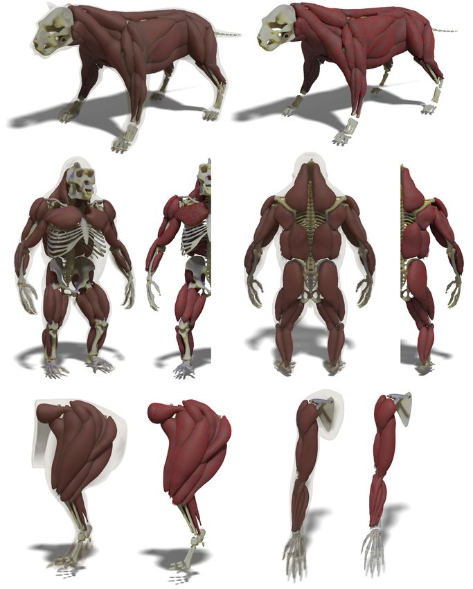
Interactive Modelling of Volumetric Musculoskeletal Anatomy • 122:11

Fig. 16. Results. We refer the reader to the provided supplemental video to see the modelling process of the Ape model. We refer the reader to the provided
Additional Modelling and Simulation Demos video to see the modelling process of the Lion model. Lion (top) and Dinosaur Leg (bottom left) are provided by
©SideFx Software. Used under permission. Ape model (middle) is obtained from https://www.3dscanstore.com/ecorche-3d-models/gorilla-ecorche-3d-model.
Used under permission. Bone geometry of the arm (bottom right) is provided by ©Ziva Dynamics. Used under permission.
 ACM Trans. Graph., Vol. 40, No. 4, Article 122. Publication date: August 2021.

122:12 • Rinat Abdrashitov, Seungbae Bang, David Levin, Karan Singh, and Alec Jacobson

6 LIMITATIONS AND FUTURE WORK can import existing muscle meshes and continue to create muscles
Although we demonstrated that our tool enables users to create around them.
complex muscular-skeletal geometries, there are limitations, subject
to future work. ACKNOWLEDGMENTS
 The quality of the muscle shapes depends on the quality of the Our research is funded in part by NSERC Discovery (RGPIN-2017-
tetrahedrazation (V,T) of the input skin and bone meshes. On one 05524, RGPIN2017–05235, RGPAS–2017–507938), NSERC Acceler-
hand, coarse meshes prevent the creation of smooth and thin mus- ator (RGPAS-2017- 507909), Connaught Fund (503114), CFI-JELF
cles; on the other hand, very high quality meshes can affect the Fund, Canada Research Chairs Program, New Frontiers of Research
performance of computing muscle functions and hinder the interac- Fund (NFRFE–201), the Ontario Early Research Award program, the
tive experience. This makes it hard to create muscles in the areas Fields Centre for Quantitative Analysis and Modelling and gifts by
where bones are too close to the skin, unless the area is densely Adobe Systems, Autodesk and MESH Inc.
tessellated. We also notice that often a large portion of the model We thank Sarah Kushner and Abhishek Madan for proofreading;
ends up being unused (the intestines area), yet it’s still being used Vismay Modi for helping to generate the simulation results; Oded
for computation of muscle functions which wastes computation. In Stein for helping with figures; anonymous reviewers for their helpful
practice, for all models, we were able to find a balance between the comments and suggestions. Special thanks to SideFx software for
quality of the tetrahedralization and performance. In the future, we providing their models.
want to explore adaptive boundary conforming tessellation of the
volume with increased tessellation quality only around boundaries REFERENCES
of the muscles. Rinat Abdrashitov, Alec Jacobson, and Karan Singh. 2019. A system for efficient 3D
 We use a simple heuristic (Sec. 3.2) for creating initial muscle printed stop-motion face animation. ACM Transactions on Graphics (TOG) 39, 1
curves, which leads to multiple editing operations of control points (2019), 1–11.
 Pankaj K Agarwal, Otfried Schwarzkopf, and Micha Sharir. 1996. The overlay of lower
to get the muscle curve shape just right. This makes it challenging to envelopes and its applications. Discrete & Computational Geometry 15, 1 (1996),
create muscle curves around complex bone geometry, since control 1–13.
points must be edited from multiple viewpoints. In the future, we Irene Albrecht, Jörg Haber, and Hans-Peter Seidel. 2003. Construction and Animation
 of Anatomically Based Human Hand Models. In Proceedings of the 2003 ACM SIG-
would like to explore a more robust curve creation techniques that GRAPH/Eurographics Symposium on Computer Animation (SCA ’03). Eurographics
simultaneously utilizes skin and bone geometry to create the best Association, Goslar, DEU, 98–109.
 Dicko Ali-Hamadi, Tiantian Liu, Benjamin Gilles, Ladislav Kavan, Francois Faure,
guess for the initial shape of the muscle curve. Olivier Palombi, and Marie-Paule Cani. 2013. Anatomy transfer. ACM Transactions
 Currently, each muscle is represented by a single curve. Based on on Graphics (TOG) 32, 6 (2013), 188.
the feedback we received from users, we plan to explore how we can Mathieu Andreux, Emanuele Rodola, Mathieu Aubry, and Daniel Cremers. 2014.
 Anisotropic Laplace-Beltrami operators for shape analysis. In European Confer-
use multiple curves to represent a single muscle. This would allow us ence on Computer Vision. Springer, 299–312.
to create more anatomically correct and complex muscle shapes with Baptiste Angles, Daniel Rebain, Miles Macklin, Brian Wyvill, Loic Barthe, JP Lewis,
multiple origin and insertion points. Additionally, there are many Javier Von Der Pahlen, Shahram Izadi, Julien Valentin, Sofien Bouaziz, et al. 2019.
 VIPER: Volume invariant position-based elastic rods. Proceedings of the ACM on
muscles in which fiber direction does not match the flow between Computer Graphics and Interactive Techniques 2, 2 (2019), 1–26.
origin and insertion and therefore we plan to explore ways to specify Autodesk 2021. Maya Muscle. http://download.autodesk.com/us/support/files/muscle.
 pdf..
the pennation angle (the angle between the longitudinal axis of the Mario Botsch, Leif Kobbelt, Mark Pauly, Pierre Alliez, and Bruno Lévy. 2010. Polygon
entire muscle and its fibers) as it is an important parameter in muscle mesh processing. CRC press.
contraction dynamics. J. E. Chadwick, D. R. Haumann, and R. E. Parent. 1989. Layered Construction for
 Deformable Animated Characters. In Proceedings of the 16th Annual Conference
 We have investigated the potential use of the resulting muscle on Computer Graphics and Interactive Techniques (SIGGRAPH ’89). Association for
geometry for simulation (Fig. 15) but more work needs to be done Computing Machinery, New York, NY, USA, 243–252. https://doi.org/10.1145/74333.
to test simulations with the complex and densely packed full-body 74358
 Nuttapong Chentanez, Ron Alterovitz, Daniel Ritchie, Lita Cho, Kris K Hauser, Ken
muscle systems. With the help of professional artists, we plan to Goldberg, Jonathan R Shewchuk, and James F O’Brien. 2009. Interactive simulation
evaluate how animation-ready our resulting muscle geometry is of surgical needle insertion and steering. In ACM SIGGRAPH 2009 papers. 1–10.
 Hon Fai Choi and Silvia S Blemker. 2013. Skeletal muscle fascicle arrangements can
using industry-standard software like Houdini [SideFx 2021] and be reconstructed using a laplacian vector field simulation. PloS one 8, 10 (2013),
Ziva Dynamics [2021]. e77576.
 Our system is designed with the idea of creating muscle geometry Barbara Cutler, Julie Dorsey, Leonard McMillan, Matthias Müller, and Robert Jagnow.
 2002. A procedural approach to authoring solid models. ACM Transactions on
from scratch but we have experimented with extracting curve net- Graphics (TOG) 21, 3 (2002), 302–311.
works from pre-existing artist-made muscle shapes (using methods Chris De Paoli and Karan Singh. 2015. SecondSkin: sketch-based construction of layered
for computing curve skeletons of 3D shapes) and importing them 3D models. ACM Transactions on Graphics (TOG) 34, 4 (2015), 1–10.
 Deepak Rajan 2021. Cassowary | Ziva Dynamics | Anatomy Modeling | Part 3. https:
into our system, which can provide a good starting point. //www.youtube.com/watch?v=AD6TAQHnZwk&ab_channel=DeepakRajan.
 We currently do not support locking of the muscle shape. How- Akio Doi and Akio Koide. 1991. An efficient method of triangulating equi-valued
 surfaces by using tetrahedral cells. IEICE TRANSACTIONS on Information and
ever, we could extract the mesh of a muscle, and treat it similarly to Systems 74, 1 (1991), 214–224.
bones so that other muscles wrap around it. This requires to redo Herbert Edelsbrunner, Leonidas J Guibas, and Micha Sharir. 1989. The upper envelope
the initial tessellation to make sure it conforms to imported muscle of piecewise linear functions: algorithms and applications. Discrete & Computational
 Geometry 4, 4 (1989), 311–336.
geometries but TetGen only takes a few seconds. Similarly an artist Gaël Guennebaud, Benoît Jacob, et al. 2010. Eigen v3. http://eigen.tuxfamily.org.
 Andrew J Hanson and Hui Ma. 1995. Parallel transport approach to curve framing.
 Indiana University, Techreports-TR425 11 (1995), 3–7.

ACM Trans. Graph., Vol. 40, No. 4, Article 122. Publication date: August 2021.