A mass-spring fluid-structure interaction solver: application to flexible revolving wings
←
→
Page content transcription
If your browser does not render page correctly, please read the page content below
A mass-spring fluid-structure interaction solver:
                                                             application to flexible revolving wings
                                                       Hung Truonga , Thomas Engelsb , Dmitry Kolomenskiyc , Kai Schneidera
arXiv:2002.08642v1 [physics.flu-dyn] 20 Feb 2020

                                                   a
                                                   Aix-Marseille Université, CNRS, Centrale Marseille, I2M UMR 7373, Marseille, 39 rue
                                                                       Joliot-Curie, 13451 Marseille Cedex 20, France
                                                   b
                                                     LMD-IPSL, École Normale Supérieure-PSL, 24 Rue Lhomond, 75231 Paris Cedex 05,
                                                                                           France
                                                       c
                                                         Japan Agency for Marine-Earth Science and Technology (JAMSTEC), 3173-25
                                                             Showa-machi, Kanazawa-ku, Yokohama Kanagawa 236-0001, Japan

                                                   Abstract

                                                   The secret to the spectacular flight capabilities of flapping insects lies in their
                                                   wings, which are often approximated as flat, rigid plates. Real wings are how-
                                                   ever delicate structures, composed of veins and membranes, and can undergo
                                                   significant deformation. In the present work, we present detailed numerical
                                                   simulations of such deformable wings. Our results are obtained with a fluid–
                                                   structure interaction solver, coupling a mass–spring model for the flexible
                                                   wing with a pseudo-spectral code solving the incompressible Navier–Stokes
                                                   equations. We impose the no-slip boundary condition through the volume pe-
                                                   nalization method; the time-dependent complex geometry is then completely
                                                   described by a mask function. This allows solving the governing equations
                                                   of the fluid on a regular Cartesian grid. Our implementation for massively
                                                   parallel computers allows us to perform high resolution computations with

                                                      Email addresses: dinh-hung.truong@univ-amu.fr (Hung Truong),
                                                   thomas.engels@ens.fr (Thomas Engels), dkolomenskiy@jamstec.go.jp (Dmitry
                                                   Kolomenskiy), kai.schneider@univ-amu.fr (Kai Schneider)

                                                   Preprint submitted to Computers & Fluids                          February 21, 2020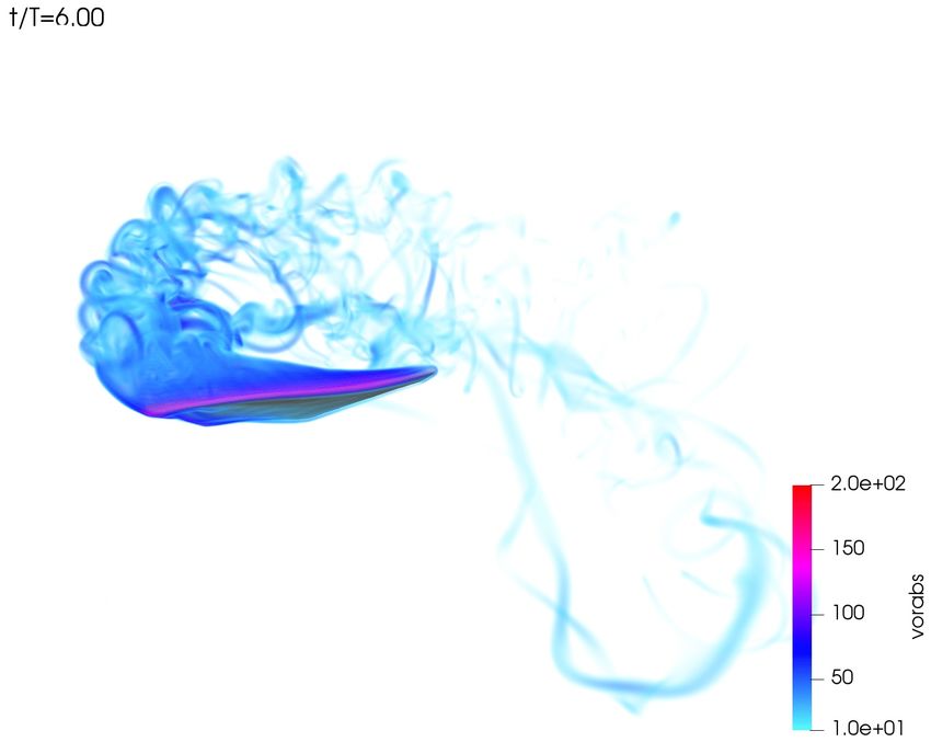
up to 500 million grid points. The mass–spring model uses a functional ap-
proach, thus modeling the different mechanical behaviors of the veins and
the membranes of the wing. We perform a series of numerical simulations of
a flexible revolving bumblebee wing at a Reynolds number Re = 1800. In
order to assess the influence of wing flexibility on the aerodynamics, we vary
the elasticity parameters and study rigid, flexible and highly flexible wing
models. Code validation is carried out by computing classical benchmarks.
Keywords:
insect flight, wing elasticity, mass–spring model, fluid–structure interaction,
spectral method, volume penalization method

1. Introduction

      A fundamental characteristics of insect flight are flexible wings, which
play an important role for their aerodynamics [1, 2, 3], requiring lower forces
than their rigid counter parts and producing reduced sound. Numerical sim-
ulation of insect flight is itself a sophisticated task, because it involves the
solution of fluid-solid interaction problems. Thus, we have to model simul-
taneously the fluid part and the solid part by using two coupled solvers.
      The fluid solver [4] we are using in the present work has been developed
previously and is called FLUSI 1 , a fully parallel software dedicated for mod-
eling three-dimensional flapping flight in viscous flows. The heart of this
software is the Fourier pseudospectral method with adaptive time stepping
used for the discretization of the 3D incompressible Navier–Stokes equations.

  1
      FLUSI:   freely   available   for       noncommercial   use   from   GitHub
(https://github.com/pseudospectators/FLUSI).

                                          2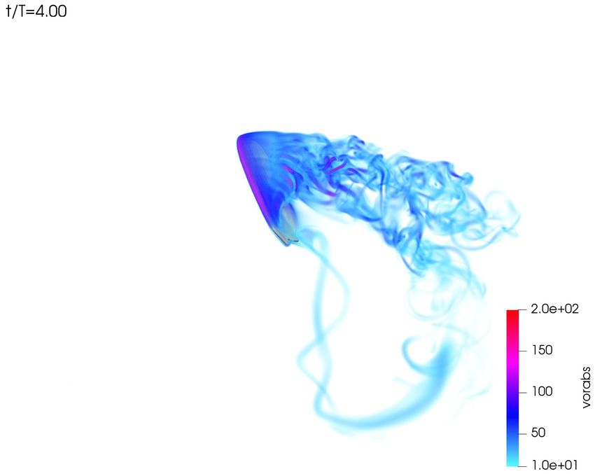
Moreover, the volume penalization method is used to take into account the
no-slip boundary conditions on the interfaces between the fluid and the solid
part.
   In [5], we performed numerical simulations of rotating triangular rigid
wings at Reynolds number Re = 250 to investigate the Leading-Edge Vortices
(LEVs) as a function of the wing aspect ratio and the angle of attack. High
resolution direct numerical simulations of rotating and flapping bumblebee
wings were presented in [6] using likewise the FLUSI code with rigid wings
focusing again on the role of LEVs and the associated helicity production.
   The interaction of flapping bumblebees with turbulent inflow in free and
tethered flight was studied in [7] using once again massively parallel com-
putations with FLUSI. We found that the fluctuations of aerodynamic ob-
servables significantly grow with increasing turbulence intensity, even if the
mean values are almost unaffected. Changing the length scale of the tur-
bulent inflow, while keeping the turbulence intensity fixed, showed that the
fluctuation level of forces and moments can be significantly reduced. We also
found that the scale-dependent energy distribution in the surrounding tur-
bulent flow is a relevant factor conditioning how flying insects control their
body orientation.
   Nevertheless, a solver for solving the deformation of the structure was
not fully developed in this software FLUSI. Hence, all previous simulations
of insect flight have been performed with the essential assumption that the
insect is composed of linked rigid parts including the wings.
   In the current work we aim at investigating the role of wing elasticity on
the flight performance. Consequently, a wing model is required for simulating

                                      3
the deformation of the solid part under the impact from the fluid. There are
many models based on continuum mechanics theory, which are used in many
well-known solid solvers. Among these, Finite Element Methods (FEM) are
mostly used in both research and industrial fields due to their reliability
and effectiveness. Despite this dominance, the requirement for faster and
more efficient methods motivates the development of alternative models. One
of these is the mass-spring system, which is known for its computational
efficiency and straightforward implementation [8]. As part of this work, a
solver using a network of masses and springs is developed to model a flexible
insect wing and coupled with FLUSI.
   The story of mass-spring models started back at the end of the 20th
century when people were dealing with observable deformations of flexible
objects in computer graphics applications, such as soft tissue, skin, hair, ball,
cloth, textiles, etc. Being considered as one of the pioneers on this field, Ter-
zopoulos et al. [9] proposed using elasticity theory for modeling deformable
objects instead of previously-used kinematic models, where the motion and
the deformation of materials were prescribed. During this period, most of
simulations of flexible objects had been calculated using finite element meth-
ods until the requirement of faster models was claimed by Eischen et al. [10].
Consequently, the development of physically based deformable models started
to grow, especially in the field of computer graphics [11] and biomedical engi-
neering [8]. While classic solvers, based on finite elements or finite difference
methods, are generally employed in the static case for computing stress and
strain in a structure, new solvers for deformable objects must have the ability
to deal with large deformations and large displacements, i.e. the nonlinear

                                       4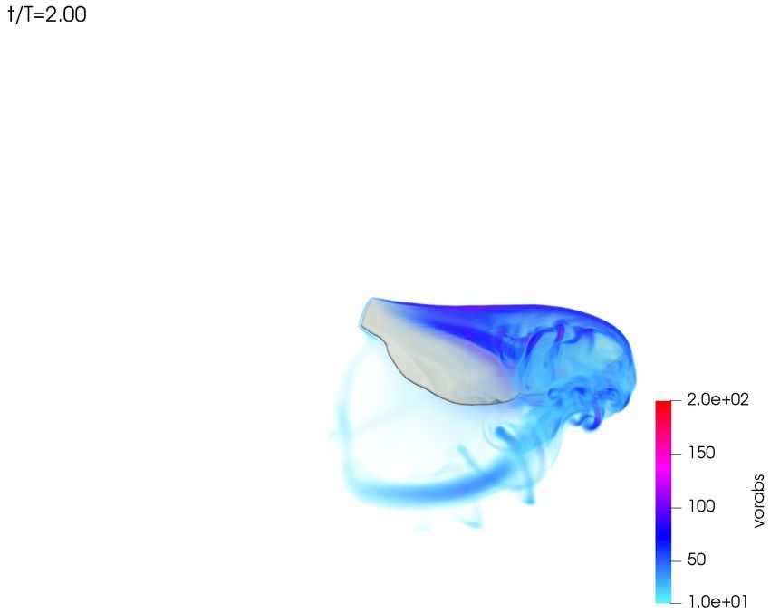
regime. Furthermore, these models need to be fast enough since they are
usually employed for real-time applications or coupled with other models
which are already time-consuming. Among all the deformable models pro-
posed, mass-spring networks stand out as the most intuitive and simplest
due to their computational efficiency [12]. Mass-spring systems have already
been employed in many fields such as medical applications [8] (muscle, red
blood cells and virtual surgery), computer graphics, fluid-structure inter-
action and insect flight. Miller and Peskin [13] used mass-spring networks
to model insect wings in two-dimensional numerical simulations. A mass-
spring network was used by Yeh and Alexeev [14] to model a flexible plate
swimmer and performed fluid-structure interaction simulation with Lattice-
Boltzmann methods in 3D. The development of our solid solver is motivated
by their mass-spring network approach, aiming to model the flexibility of
insect wings in the three-dimensional case.
   The goal of this paper is to move from rigid to flexible wings and to
present a fluid-structure interaction solver for flapping flight, based on the
open access software FLUSI, where we integrated a solid model based on
mass-spring systems. However, the wing kinematics of insects is very diffi-
cult to obtain, since the measurements usually require high tech equipment
to capture all the dynamic motion at small time scale and length scale. In-
stead, a revolving wing model is usually employed to study the aerodynamics
of flapping wings thanks to its simplicity. Accordingly, the flow fields and
force generation aspects of revolving wings have been analyzed for a wide
range of parameters, as reported in the literature [15, 16, 17]. Di et al. [18]
studied the role of forewings in generating LEVs of three revolving insect

                                      5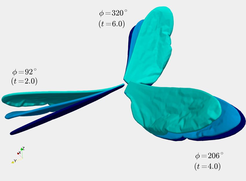
wing models: hawkmoth (Manduca sexta), bumblebee (Bombus ignitus) and
fruitfly (Drosophila melanogaster). Van de Meerendonk et al. [19] inves-
tigated experimentally the flow field and fluid-dynamic loads of a flexible
revolving wing to quantify the influence of flexibility on the force generation
performance of the wing. In our study, we also consider revolving flexible
bumblebee wings and assess the influence of the wing deformation.
   The outline of this paper is the following: In sec. 2 we present a mass-
spring model for describing the flexible insect wings. The wing structure
of the considered bumblebee wings and its mass distribution are detailed in
sec. 3. The numerical artillery of fluid-structure interaction is explained in
sec. 4 and some validation tests are given. The numerical results as well
as the discussion about the influence of the flexibility on the aerodynamic
performance are presented in sec. 5. Finally, conclusions are drawn in sec. 6,
including some perspectives for future investigations.

2. Flexible wing

2.1. Mass-spring model

   The very basic idea of the mass-spring model is to discretize an object
using mass points mi (i = 1, ..., n) connected by springs. There exist many
kinds of springs for different purposes but in the limit of our work, we have
used only linear extension and bending springs to model insect wings. The
dynamic behavior of the mass-spring system, at a given time t, is defined by
the position xi and the velocity vi of the mass point i. For this, we need
to solve the dynamic equations of the system, which govern their motion in
time under certain external forces. This is one of the elegant advantages

                                      6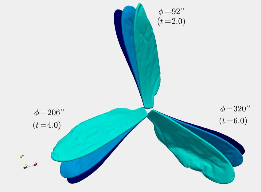
of the mass-spring network where these governing equations are simply the
corresponding classical well-known Newton’s second law, given in eqns. (1).

                         Fi = mi ai

                         Fi = Fint  ext
                               i + Fi          for i = 1...n
                                                                           (1)
                  vi (t = 0) = v0,i

                  xi (t = 0) = x0,i

where n is the number of mass points, Fi is the total force (internal force
Fint
 i   and external force Fext
                         i ) acting on the i
                                            th
                                               mass point, mi , ai are mass
and acceleration of the ith mass point, respectively.
   Here, all terms are quite simple to derive except for the forces. The exter-
nal forces come from outside of the system and depend on the surrounding
field and the problem we are dealing with. On the other hand, the internal
forces represent the restoring forces caused by the springs. The complicated
properties of these forces make the system (1) become nonlinear. Hence, we
have a nonlinear system of 3n second order ordinary differential equations
(ODEs) corresponding to three dimensions x, y, z and n mass points. In the
general case, this system (1) needs to be solved numerically since its analyti-
cal solution cannot be derived. In practice, it is more convenient to convert a
system of 3n second order equations into a system of 6n first order equations
by using the relations ai = dvi /dt and vi = dxi /dt. Eqns. (1) can then be

                                      7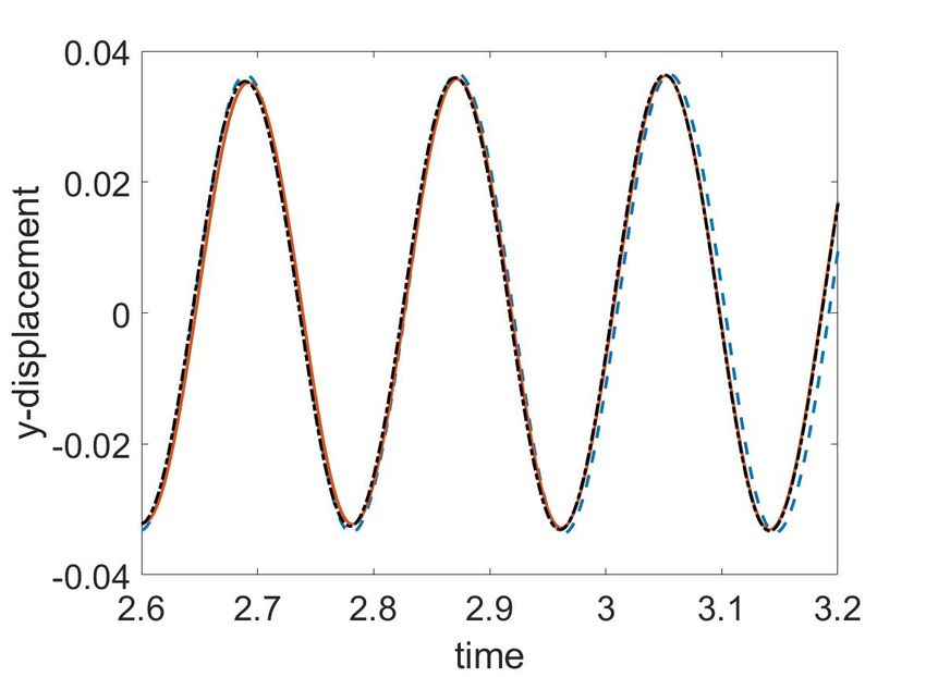
rewritten as below:
                         dxi
                             = vi
                          dt
                         dvi
                      mi     = Fint  ext
                                i + Fi            for i = 1...n
                          dt                                               (2)
                  vi (t = 0) = v0,i

                  xi (t = 0) = x0,i
                      |
Let us call q = xi , vi the phase vector containing positions and velocities
                                                 ext |
of all mass points and f (q) = vi , m−1
                                         int

                                     i (Fi + Fi )      the right hand side
function, eqns.(2) can be rewritten again under the familiar form of a system
of first order ODEs as follows:
                                      dq
                                         = f (q, t)
                                      dt                                   (3)
                               q(t = 0) = q0

For time stepping, eqns. (3) need to be discretized using an appropriate
numerical scheme. The choice for this scheme is not trivial since it depends
on many factors. Due to the size of the wings, the mass-spring network
contains a lot of very small springs, which make the system very stiff and we
need an implicit scheme for time marching. For this reason, either a centered
scheme or a backward scheme can be used. Although centered schemes are
usually in favor for their conservation property without numerical diffusion,
a centered scheme, for example the trapezoidal scheme, can lead to numerical
instability at some points because the eigenvalues of the operator of the time
discretization lie exactly on the imaginary axis, the boundary of the stability
zone [20]. Furthermore, the coupling between the fluid and the solid solver
will require an adaptive time stepping scheme. For all these reasons, a second

                                        8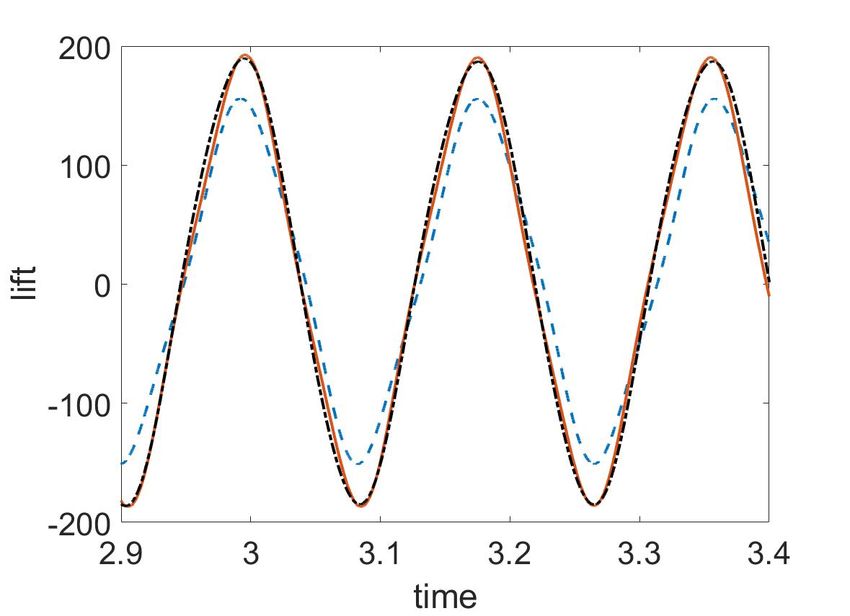
order backward differentiation scheme with variable time steps [21] is used
to discretize eqns. (3) in time.

                    (1 + ξ)2 n     ξ2           1+ξ
           qn+1
            i   −           qi +        qn−1
                                         i   =        ∆tn f (qn+1
                                                              i   )        (4)
                     1 + 2ξ      1 + 2ξ        1 + 2ξ

where ξ = ∆tn /∆tn−1 is the ratio between the current ∆tn and the pre-
vious time step ∆tn−1 . Eqn. (4) is a system of nonlinear equations with
the variable qn+1 , the phase vector of the system at the current time step,
which needs to be solved. The Newton–Raphson method, a powerful itera-
tive method, is employed to solve this nonlinear system of equations. With
an initial guess, which is reasonably close to the true root of the equations,
Newton–Raphson helps to find approximations of the root with the rate of
convergence estimated to be quadratic. For our mass-spring solver, the ini-
tial guess chosen is the phase vector qn solved at the previous time step; this
allows the Newton–Raphson method to converge quickly since the structure
is advanced slowly and smoothly in time, which assures that qn+1 remains
close to qn . In most cases, the Newton–Raphson method in the solver needs
three to four iterations to converge within a relative or absolute L2 norm
error of 10−6 as the stopping criterion.

2.2. Extension springs and bending springs
   Extension springs (figure 1a) and bending springs (figure 1b) are common
mechanical devices, which resist against the external forces to get back to
their resting positions. The former is designed to operate with axial forces,
while the latter is used for torques. The relations between the displacement
and the restoring force are given by:

                                        9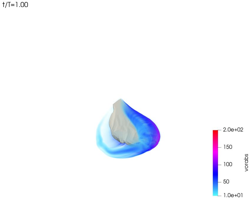
• Linear extension spring

                             Fi = kije (||xij || − ||x0,ij ||) eij
                                                                                (5)
                             Fj = −Fi

     where kije is the extension stiffness, eij = (xj −xi )/||xj − xi || is the unit
     position vector and Fi and Fj are the restoring forces of the extension
     spring acting on two points i and j, respectively;

   • Linear bending spring

                                       b
                              Mijk = −kijk (θijk − θ0,ijk )                     (6)

     or in terms of forces

                             b
                       Fi = kijk (θijk − θ0,ijk ) (eij × ejk ) × eij
                            b                                                   (7)
                      Fk = kijk (θijk − θ0,ijk ) (eij × ejk ) × ejk

                       Fj = −Fi − Fk

                                          b
     where Mijk is the restoring moment, kijk is the bending stiffness, θ0,ijk is
     the initial bending angle among three points i, j and k, θijk the current
     bending angle and Fi , Fj , Fk are the restoring force vectors (as shown
     in figure 1) of the bending spring acting on three points i, j and k,
     respectively.

   However, the calculation of θijk in eqn.(7) is not trivial since it involves
the geometrical definition of the angle in 3D space with respect to a fixed

                                          10
coordinate system. Firstly, we consider a simpler case when the three points
are in the same plane, a 2D coordinate system Oxy. This leads to xi =
(xi , yi )T , xj = (xj , yj )T and xk = (xk , yk )T . The angle is now determined by:
h
θijk = atan2 (yk − yj )(xj − xi ) − (yj − yi )(xk − xj ),
i (8)
(xk − xj )(xj − xi ) + (yk − yj )(yj − yi )
Here, atan2 (usually known as two-argument arctangent) is a special func-
tion first introduced in computer programming languages to give a correct
and unambiguous value for the angle by taking into account the sign of both
arguments. This function helps us to calculate on the whole space when the
angle can vary in the range of (−π, π], instead of the range of (−π/2, π/2)
when using the standard arctangent function.
For a problem in 3D space, only one bending angle will not be sufficient.
This can be easily seen by considering a simple case of one bending spring.
At an instant t, the spring is deformed and has a bending angle θijk . Nev-
ertheless, corresponding to this θijk , there is an infinite number of solutions
xi , xj and xk that can satisfy this deformation and the set of all these so-
lutions forms a cone, like shown in figure 2. Consequently, one more angle
is needed to obtain a unique solution. To define these two bending angles,
the same bending spring as the 2D case above is considered but now in a 3D
coordinate system Oxyz. The bending spring is projected on the Oxy and
y z
the Oxz planes which gives us two 2D bending angles θijk and θijk on the
Oxy and the Oxz planes, respectively. Then, like in the 2D problem, these
two bending angles are calculated as below:
11h
y
θijk = atan2 (xj − xi )(yk − yj ) − (xk − xj )(yj − yi ),
i
(xj − xi )(xk − xj ) + (yj − yi )(yk − yj )
h (9)
z
θijk = atan2 (xj − xi )(zk − zj ) − (xk − xj )(zj − zi ),
i
(xj − xi )(xk − xj ) + (zj − zi )(zk − zj )
2.3. Functional approach - vein and membrane models
Modeling insect wings is challenging due to the fact that these wings
have complex structures composed of a network of veins, partly connected
through hinges, with thin membranes spanned in between and their elastic-
ity properties are still poorly understood. Certain studies have shown that
the vein arrangements in insect wings have strong impact on their mechan-
ical properties [3, 22]. Thus, it will be inaccurate to consider a wing as a
homogeneous structure; the vein pattern as well as the difference in terms
of mechanical behaviors between vein and membrane need to be taken into
account. However this is not an easy task, since insects are the most diverse
group of animals living on Earth with more than one million known species
with varying wing sizes and wing shapes. As a result, in this study, we want
to limit ourself to a specific case when we examine only bumblebee (Bombus
ignitus). Bumblebee wings are mainly composed of veins and membranes.
The longitudinal veins extending along the wing in the spanwise direction
are big, hollow and providing conduits for nerves while the cross veins are
smaller, solid and connecting the longitudinal veins to form a kind of truss
structure. In the space between these veins, we find a thin layer called mem-
brane.
12From a mechanical point of view, veins can be considered as rods which
resist mainly the torsion and bending deformation. On the other hand, a
membrane is fabric-like, it behaves like a piece of cloth which resists again
the extension deformation. Consequently, instead of considering the wing as
a homogeneous structure, a functional approach is used to distinguish veins
and membranes. We then propose two models using mass-spring networks
to imitate the mechanical behavior of the vein and the membrane.
A vein is considered as a rod whose length is much greater than its height
and width. The total effect of all the external loads applied on a mechanical
structure results in deformation which can usually be classified into three
main types: bending, twisting and stretching. Although the whole wing is
observed to be twisted significantly in many studies using high speed cameras
or the digital particle image velocimetry [23, 24, 25, 26, 27], it is not entirely
clear that torsion happens locally at veins or the unsynchronized bending
deformations between veins cause the whole wing to twist. To simplify the
model, we study only the latter in which we ignore the local torsion of veins
and model solely the bending deformation of veins by using extension and
bending springs. Thus, we model a vein by a curve line which is discretized by
n mass points as shown in figure 3. Two neighboring points are connected
with each other by an extension spring (e.g. the mass points i and i + 1
are connected by the extension spring kie ) and three neighboring points are
connected with each other by a bending spring (e.g. the mass points i − 1, i
b
and i + 1 are connected by the bending spring ki−1 ).
When flapping, most of external forces will act in the direction perpen-
dicular to the wing surface. As a result, the stretching deformation is negli-
13gible comparing to the bending deformation. Thus, the role of the extension
springs in the model is solely to conserve the length of the vein. The stiffness
of these extension springs is artificial and they do not need to reflect the
mechanical property of the vein itself. They should be chosen stiff enough to
make the rod unstretched but not too stiff to avoid problems with numerical
stability when integrating the dynamical system in time.
Compared to veins, membranes are totally different in terms of geomet-
rical and mechanical properties. Geometrically, a membrane is an object
whose thickness is much smaller than its extent. Consequently, a membrane
is usually considered as a planar two-dimensional sheet or a set of planar
sheets in the case of non-planar three-dimensional membranes [28, 29]. On
the mechanical side, a membrane is a special kind of structure compared to
other structural elements, i.e. a rod, a bar, a plate or a beam. It behaves
like a piece of cloth which is much easier to be bent than to be stretched
or compressed. Keeping these in mind, the membrane part of the wing is
modeled by a 2D sheet which is discretized by a system of mass points and
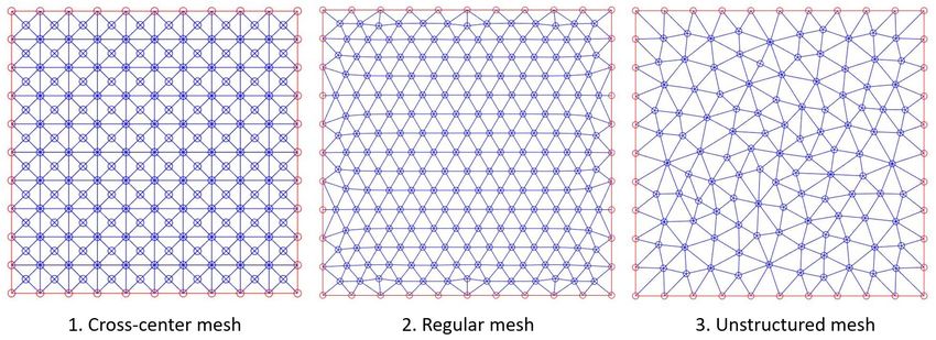
extension springs. There are several ways to discretize a 2D sheet (as shown
in figure 4) but an unstructured triangular mesh needs to be employed for
our problem due to the complicated geometry of insect wing. Moreover, an
unstructured mesh is preferred for modeling isotropic membranes [30] since
the random orientations of the springs will average out the forces.
2.3.1. Correlation between mass-spring network models and continuum con-
stitutive laws
Besides the mesh topology, the parameter setting is another challenge
that one has to solve in order to correctly model the material of which the
14object is made. There are two main parameters needed to be assigned for a
mass-spring model: the masses and the spring stiffness. Although a Voronoi
diagram can be used to find the masses in a proper way [32], selecting spring
stiffness is still an open question and there are two common solutions to
overcome this [33]. The first approach is based on optimization methods to
minimize the difference between the results solved by the mass-spring model
and the reference data. These reference data can come from the measure-
ments, the visual appearance of real objects [34] or numerical solutions using
validated methods such as finite element methods [35, 36]. In general, this
approach cannot be applied if the system has too many degrees of freedom
with many unknown spring constants or the mesh topology varies in time
since one set of parameters works for solely one mesh structure. Otherwise,
tuning the spring stiffness by using optimization can give satisfying results
with reasonable computational cost.
The second way is about deriving a relation between spring stiffness and
other continuum mechanic properties, such as Young modulus, the Poisson
ratio and the flexural rigidity. In contrast to the discrete models, the elas-
ticity parameters have been obtained for many materials and can be used
to calculate the corresponding spring stiffness. Omori et al. [31] succeeded
in doing this for a planar membrane by considering a 2D sheet under small
uniaxial deformation. The relation between spring networks and continuum
models for three types of meshes is shown in figure 5.
For the vein model, a relation between the flexural rigidity EI and the
stiffness of the bending springs kib is needed. To derive this relation, we
consider a classical problem of a cantilever beam length lb , under a point
15force F at the free end (figure 6). In the limit of small displacement, the
principle of energy yields the value of the bending spring stiffness k b as a
function of the flexural rigidity EI. The energy stored in this beam at the
static state can be calculated easily using the Euler-Bernoulli beam theory
as shown in eqn. (10).
F 2 lb3
Ebeam = (10)
6EI
The mass-spring network is called an equivalent model of the continuous
beam if under the same external loads, its mechanical behavior (in this case, it
is the energy stored in the system) is the same as the one of the beam. Let us
now study a mass-spring network discretized into n+2 mass points connected
by bending and extension springs as shown in figure 6. All the bending and
extension springs are the same with a stiffness k b and k e , respectively and
k e
k b . The first two points are totally fixed to represent the boundary
condition of the fixed end of the beam. Writing the equilibrium equations
for the remaining n points, we have:
lb
F (n + 1 − i) = k b (θi+1 − θi ) for i = 1...n (11)
(n + 1)
Considering the deformations of extension springs are very small, the
total potential energy of all the bending springs of the system is
n
1 X
Emass−spring = kb (θi+1 − θi )2 (12)
2 i=1
With eqn. (11) and eqn. (12) we obtain:
16n
F 2 lb2 X
Emass−spring = b i2
2k (n + 1)2 i=1
F 2 lb2 n(n + 1)(2n + 1) (13)
= b 2
2k (n + 1) 6
2 2
F lb n(2n + 1)
=
12k b n + 1
By comparing eqn. (10) and eqn. (13), we can derive an analytical
relation between kb and EI as following:
EI n(2n + 1)
kb = (14)
lb 2(n + 1)
Since eqn. (14) is derived based on the assumption of small displacement,
we still have here a linear problem thus the principle of superposition can
be applied. During the flight, the aerodynamic loads acting on insect wings
can be considered to be equivalent to distributed loads on the surface of
the wings. These distributed loads can be discretized into many point forces
using a work-equivalent method [37] and then the superposition principle can
be applied. Thus, it is sufficient to analyze only one point force case to find
the relation between EI and k b , since it does not depend on the point force
F.
However, as mentioned at the beginning of this section, insect wings are
deformed significantly to create lift for flying. Here, we are dealing with a
large displacement problem and the question is if eqn. (14) still remains valid.
The technique used to derive (14) is no longer applicable since the solution
for large deflection of a cantilever beam cannot be obtained analytically [38].
This problem involves calculating elliptical integrals of the second kind [39]
17and needs to be solved numerically. Consequently, the relation between EI
and k b is put into a large displacement, nonlinear test case to check if we
still get the same mechanical behaviors between the continuous beam and
the mass-spring model. The results are presented in the next section.
2.4. Validations of the mass-spring model
2.4.1. Vein model - Cantilever beam under gravitational force
Static case. Firstly, we consider a static case of a cantilever beam with length
L = 0.3, flexural rigidity EI = 0.24 and loaded by a point force F at the
free end. The force F varies from 0.39 to 11.76 and it must be strong enough
to cause a large deflection. All the parameters here are dimensionless. The
vertical displacement δy and the horizontal displacement δx of the free end
of the beam at equilibrium state can be calculated by using the fundamental
Bernoulli–Euler theorem [40] and the mass-spring network as given in table
1.The static state of the vein model (discretized by n = 64 mass points)
is obtained by solving the dynamic equations of the system with artificial
damping forces to make the system go quickly towards its balanced position.
Despite the small displacement assumption for deriving the relation between
EI and k b , the relation in eqn. (14) is still valid even in very large deflection
problem. For the case F = 3.92, the vertical displacement of the free end is
already more than 30% of the total length of the beam and we still get very
good agreements between both models with the relative error being smaller
than 1%. The mapping from EI to k b can then be generalized for nonlinear,
large deflection cases with good agreement between the continuum theory
and the discrete mass-spring network.
18Table 1: Comparison between the continuum theory and the discrete mass-spring network
in the static large deflection case.
Point force Nonlinear beam [39] Mass-spring network Relative error
F δxref [10−2 ] δyref [10−2 ] δx[10−2 ] δy[10−2 ] errx [%] erry [%]
0.39 29.96 -1.46 29.96 -1.46 0 0
1.96 29.02 -6.93 29.01 -6.92 0.03 0.14
3.92 26.87 -12.14 26.85 -12.1 0.07 0.33
7.84 22.53 -17.93 22.53 -17.85 0 0.45
11.76 19.37 -20.69 19.40 -20.57 0.15 0.58
Dynamic case. The vein model will now be compared with another solid
solver developed by Engels et al. [41]. It is based on the classical nonlinear
beam equation, the Euler–Bernoulli theory. All details about this solver can
be found in [20]. We study the case when we have a 2D cantilever beam
(figure 7) of length lb = 1, density ρ = 0.0571, flexural rigidity EI = 0.0259.
The beam is in vacuum, subjected to a gravity field g = 0.7 strong enough
to cause large deflection. All the parameters here are dimensionless. Both
computations are performed for the same numerical parameters with the time
step dt = 10−2 and n = 64 grid points. Although both solvers require the
same amount of CPU time for the same resolution, the mass-spring network
is still more efficient since it is designed to deal with 3D problems. For
the computation, the mass-spring solver handles a system of 3n degrees of
19freedom, corresponding to 3 dimensions, while the nonlinear-beam solver
only solves for 2n variables.
The deflection line of the two models at a given time t and the oscilla-
tion of the trailing edge yte (t) are shown in figure 8. The dashed blue line
calculated by the nonlinear beam theory and the solid red line calculated by
the mass-spring network are almost coincident with each other. We have an
excellent agreement between these two models with a relative error smaller
than 1%.
2.4.2. Membrane model - Uniaxial and isotropic deformations of a two-dimensional
sheet
We consider here the same test case proposed by Omori et al. [31] where
a square 2D sheet with an initial side length l0 = 1 is extended by a uniaxial
tension T = 0.005 and has a final length l in the x-direction at the equilibrium
state, as shown in figure 4. This tension must be small enough to cause small
deformation on the sheet. The Young modulus Es is defined by:
T
Es = (15)
where is the strain.
The sheet is then discretized by using three types of meshes, illustrated
in figure 4. The grid size ∆l is the side length of one triangle element of the
mesh and inversely proportional to the number of grid points n. The grid
size is varied to refine the mesh resolution. Since we are only interested in
the equilibrium state of the model, the masses will not have any effect on the
result and they are chosen properly for the numerical convergence. Instead
of solving the static equation of the system, we still solve here the dynamic
20equations of the system with artificial damping forces to make the system
go quickly towards its balanced position. Last but not least, all the spring
stiffnesses are set to the same value k = 1. Figure 10 shows the results we get
for all three mesh structures. First, for the cross-center structure, we are able
to reproduce the result of Omori et al. [31]. When the mesh is refined, the
ratio k/Es converges to the analytical value 3/4 with the relative error being
smaller than 1%. For the regular triangle, due to the shape of the square, we
have some minor flaws of the mesh at the border. But these can be neglected
when the mesh is fine enough and we can consider it as a regular triangular
mesh. Indeed, for high resolution, we find again an excellent agreement with
√
the analytical ratio k/Es = 3/2 derived by Omori et al. The relative error
is also smaller than 1%. However, for the unstructured mesh, the convergent
value of k/Es is larger than the one of Omori et al., but identical to the
analytical solution for the regular triangle. This finding is in fact expected
by Omori et al. since these two meshes are both constructed with triangles,
each node being connected to six springs. Yet, the random structure of the
unstructured mesh makes it difficult to explain the difference.
Using our mass-spring model, we are capable of reproducing the results
from the references, which indicates the reliability of the solver. These re-
sults for both small and large deformation cases allow us to have the same
conclusions as in the literature about the mass-spring system. Even though
the mechanical properties of spring networks are strongly dependent on the
mesh topology, a correlation between the discrete model and the continuum
model can still be obtained if the mesh is fine enough. However, this needs to
be compromised with the computational efficiency which is the main reason
21that we choose mass-spring network in the first place.
3. Wing structure
The simulation of insects with flexible wings is extremely complicated
not only because it involves solving for both fluid and solid dynamics, but
also due to the fact that insect wings are sophisticated structures. In our
work, we want to take into account as much as possible all the mechanical
properties of the bumblebee wing, in order to correctly model its dynamic
behaviors. In our wing model there are three main factors introduced, which
are considered to have the most impact on wing deformation during flight:
venation pattern, mass distribution and vein stiffness.
3.1. Venation pattern
The venation architecture is claimed to affect the anisotropy of the wing.
Throughout measurements from different insects, Combes et al. [3, 22] sug-
gest that wing flexural stiffness declines exponentially towards the tip and
trailing edge. This is explained by the common venation patterns of insect
wings: most insect wings have thick, stiff veins at the leading edge and cross
veins are thinner as they expand toward the wing tip. This structure allows
insect wings to resist against strong bending deformation in the spanwise
direction, while creating camber for lift generation in the chordwise direction
[22]. Nakata and Liu [2] modeled the anisotropy caused by wing veins. To
this end they took into account the variation of wing thickness and intro-
duced a ”rule of mixture” of composite materials.
In our model, the functional approach is used to take into consideration
the venation pattern. The vein structure, as well as the wing contour, are
22adapted from the data from [42] and encoded into the mass-spring network,
as shown in figure 11. Comparing to the reference data, two more veins are
added (vein 21 in the forewing and vein 7 in the hindwing) and two forewing
veins 19 and 20 are extended toward the tip of the wing. These modifications
are made to add bending stiffness to the tip of the wing and thus to obtain
a more realistic behavior during the simulation. The meshing is done by
identifying firstly the contour of the wing and all the veins (green, red and
blue curves in figure 11). The membrane is then discretized by a triangular
mesh using SALOME 2 , an open-source integration platform for numerical
simulation and mesh generation.
3.2. Mass distribution
Another property which plays an essential role on the aerodynamics of the
wing, is the mass distribution. It represents the inertia of the system and the
position of the mass center has a strong connection with the stability of the
wing during flight. The mass distribution is calculated based on the measured
wing mass data from [42]. For our numerical simulations, the total wing
mass is chosen as the same used by Kolomenskiy et al. [42], mw = 0.791 mg.
The mass is then distributed into vein and membrane parts based on their
geometry and material. Each vein is considered as a rod composed of cuticle,
ρc = 1300 kg/m3 [42], with a circular cross section of constant diameter dv
[42] and length lv , calculated directly from the model. The mass of each
vein is then calculated and shown in table 2. Both diameter and mass are
dimensionless quantities, normalized by wing length L and air density ρair L3 ,
2
https://www.salome-platform.org/
23respectively.
The mass distribution for the membrane is more tricky since we do not
have the material properties of bumblebee membranes. A bi-linear regression
is employed due to the fact that the membrane is heavier near the wing
root and the leading edge [42]. An optimization is employed to find the
parameters for the regression using the mass center from the measured data
as an objective function. For a mass point mi belonging to the membrane at
position [xi , yi ] (the z coordinate is neglected here because we assume that
the membrane is a planar sheet), we get:
mi = 1.75 · 10−4 − 2.83 · 10−4 xi + 4.91 · 10−4 yi (16)
This yields a difference, between two mass centers, of 0.0013 in the x-direction
and 0.0085 in the y-direction which are really small compared to the reference
wing length Rw = 1.
3.3. Vein stiffness estimation
To study the influence of wing flexibility on the aerodynamics perfor-
mance, the flexural rigidity of veins will be changed to alter the bending
stiffness of the wing. Consequently, only Young modulus E will be varied.
Insect cuticles are reported to have a Young modulus about 1kP a to 50M P a
[43]. For our study, we are choosing two values of E (corresponding to flexible
and highly flexible wings): 3.5 kP a and 35 kP a, which are in this range and
give realistic deformations comparing to those observed in real life. Then, the
flexural rigidity EI of each vein will be calculated using the second moment
of inertia I of circular-section veins with diameters given in table 2.
24Forewing Hindwing
Nominal Nominal Nominal Nominal
# #
diameter mass diameter mass
1 0.0070 0.0209 1 0.0065 0.0180
2 0.0074 0.0237 2 0.0043 0.0071
3 0.0055 0.0076 3 0.0046 0.0024
4 0.0070 0.0063 4 0.0011 0.0001
5 0.0040 0.0031 5 0.0038 0.0043
6 0.0048 0.0094 6 0.0037 0.0005
7 0.0040 0.0019 7 0.0020 0.0012
8 0.0038 0.0009
9 0.0041 0.0023
10 0.0048 0.0064
11 0.0045 0.0017
12 0.0038 0.0018
13 0.0042 0.0010
14 0.0038 0.0020
15 0.0034 0.0008
16 0.0032 0.0005
17 0.0032 0.0004
18 0.0044 0.0009
19 0.0015 0.0001
20 0.0018 0.0001
21 0.0020 0.0009
Table 2: Dimensionless vein diameter dv (adapted from [42]) and their corresponding
dimensionless mass mv .
254. Fluid-structure interaction
4.1. Numerical method
The ultimate goal of this work is the fluid-structure interaction simulation
of insects with flexible wings. To study the airflow as well as the effect
of flexibility on the aerodynamic performance of the wing, the developed
mass-spring model needs to be coupled with a fluid solver. This is done by
combining the volume penalization method [44] with a Fourier pseudospectral
discretization [45], for which we developed the parallel opensource solver
FLUSI, freely available on Github3 [4]. The code solves the incompressible,
penalized Navier-Stokes equations
χ 1 (χsp ω)
∂t u + ω × u = −∇Π + ν∇2 u − (u − us ) − ∇× (17)
C C ∇2
| η {z } | sp {z }
penalization term sponge term
∇·u=0 (18)
u(x, t = 0) = u0 (x) x ∈ Ω, t > 0 (19)
where u is the fluid velocity, ω is the vorticity, Π = p + 21 u · u is the total
pressure, ν is the kinematic viscosity. We find here again all the familiar
terms of the classical Navier–Stokes equations except for the sponge and pe-
nalization terms. The former is a vorticity damping term used to gradually
damp vortices and alleviate the periodicity inherent to the Fourier discretiza-
tion. The last term is used to impose the no-slip boundary conditions on the
fluid-solid interface as explained in [4]. All the geometry information of the
3
https://github.com/pseudospectators/FLUSI
26solid is encoded in the mask function χ, which is usually taken as one inside
the solid and zero otherwise. However, we are dealing with a moving flexible
obstacle and the discontinuous mask function χ need to be replaced by a
smooth one, eqn. (20), to avoid oscillations in the hydrodynamic forces [20].
Thus, we employ a mask function χ as shown below:
δ ≤ tw − h
1
χ(δ) =
1
2
1 + cos π (δ−t2h
w +h)
tw − h < δ < tw + h (20)
0 δ ≥ tw + h
where h is the semi-thickness of the smoothing layer, tw is the semi-thickness
of the wing and δ is the distance function which gives us the distance from
Eulerian fluid nodes to the center surface of the wing. As presented in section
3, an unstructured triangular mesh is employed for our wing model. Thus,
the discretized wing surface is composed of triangles constructed by three
vertices (e.g. xs,i , xs,j and xs,k ). The distance function δ is computed by
cycling over all these triangles. Since we are only interested in the fluid
nodes near the fluid-solid interface, a bounding box is used to save computing
time. For each triangle, the distance from it to all the fluid nodes belonging
to its bounding box will be computed by using the algorithm from [46]. The
distance function at one fluid node is finally the minimum distance from this
fluid node to all the triangles nearby.
δ(x, t) = min(||x − triangle(xs,i , xs,j , xs,k )||2 ) (21)
The solid velocity field us is calculated in the same way as the distance
function δ. If the triangle (xs,i , xs,j , xs,k ) is the one closest to the fluid node
27x, x will be projected onto the plane of the triangle and the solid velocity
of the projected point is interpolated from the velocities of the three vertices
by using barycentric interpolation. Because we do not consider the flexibility
of the wing in the direction perpendicular to the wing surface, the velocity
of the projected point should be the same as the one of the fluid node.
Nevertheless, the solid velocity field is defined in the global reference frame
for the fluid solver while the velocity solved by the solid solver is in the local
wing reference frame. These velocities are needed to be transformed back
to the global reference frame using eqn. (22) where VO(w) and Ω are the
translating and rotating velocity of the wing reference frame, v(w) and x(w)
are the velocity and the position computed by the solid solver in the wing
reference frame, respectively.
us = VO(w) + v(w) + Ω × x(w) (22)
Moreover, the fluid also interacts with the wing via the pressure and
viscous force. However, at Re = O(103 ) in our study, the viscous force
is considered to be very small and only the pressure force is transferred
into the mass-spring system as external force. Contrary to the previous
calculation of the solid velocity field us , the pressure force is interpolated
from the Eulerian fluid grid onto the Lagrangian mass points. The pressure
interpolation is quite straightforward because the pressure field solved by the
penalized Navier–Stokes equations is following the Darcy law and continuous
even inside the wing [44]. Consequently, the pressure at any mass point can
always be determined, using delta interpolation proposed by Yang et al. [47],
from pressure values at neighboring Eulerian grid points [20]. Then for each
28triangle element of the wing, the pressure forces at the three vertices are
perpendicular to the triangle and have magnitudes equaling to the pressure
multiplied by one third of the triangle area. This is done for all the triangles
and then accumulated to obtain the overall external pressure forces acting
on the mass-spring system.
For time-stepping, the coupled fluid-solid system is advanced by employ-
ing a semi-implicit staggered scheme as proposed in [20]. At time step tn ,
the fluid velocity field is advanced to new time level un → un+1 from the old
mask function χn and the old solid velocity field uns by using the Adams–
Bashforth scheme. Then, the pressure field at the new time step pn+1 is
calculated from the fluid velocity field un+1 . Finally, the solid is advanced
to the new time step χn+1 and un+1
s and the whole process is repeated until
the final time.
4.2. Validation
For the validation of the fluid-solid coupling, we consider two test cases:
the Turek benchmark test case FSI3 [48, 49] and the rigid revolving bumble-
bee wing test case [6].
4.2.1. Turek benchmark FSI3
The Turek benchmark FSI3 involves a flexible appendage of length l =
0.35 and thickness h = 0.02 placed right behind a circle cylinder of radius
R = 0.05; the whole obstacle is immersed in a channel of size H × L =
0.41 × 2.5 with a Poiseuille inflow of meanflow Ū = 2, as shown in figure 12.
The center of the cylinder is placed a bit lower to the centerline at (0.2, 0.2)
to trigger the instability and to make the appendage oscillate.
29The fluid solver, as well as the fluid-solid coupling, are handled by the
software FLUSI [4] and the setup remains the same as the test case FSI3
with a resolution of 5200 × 1152 whose details can be found in [20]. Only
the solid solver based on the nonlinear beam equation, which is used for
validation in section 2, is now replaced by the new solver using the mass-
spring network for validation. The results of this simulation are presented
in table 3 for the comparison with the reference solutions presented in the
literature [20, 48, 49].
For the oscillation of the trailing edge yte , the result is in excellent agree-
ment with all three references when the maximum relative error, for both
maximum and minimum values of yte , is only 1.76% and the relative error
for the frequency of oscillation is 1.65%. The vertical displacement of the
trailing edge with respect to time in the periodic state is also plotted in
figure 13 to compare with the reference [49]. The two lines are almost super-
posed on each other. Nevertheless, the computed drag is less accurate with
a relative error which can go up to 4.57% comparing the maximum value
with the reference [20], but only 1% comparing with [48]. From figure 13,
the curves of the two solutions appear to have the same shape but have some
offset. This offset is explained in [20] to be due to the smoothing layer in
the mask function, which plays a role as surface roughness. This leads to the
over-prediction of the drag force. Concerning the lift force, the mass-spring
model yields results very close to the one calculated by Engels with the error
of 2.76%, and the difference is around 20% with respect to [48, 49] for both
max and min values. Like in Engels [20], the amplitude of the lift force is
over-predicted by coupling FLUSI and the mass-spring solver. In conclusion
30References yte [10−3 ] Drag Lift f0
max min max min max min
Mass-spring network 36.22 -32.93 503.02 442.12 189.94 -186.23 5.56
(1) T. Engels [20] 35.63 -32.71 481.20 432.50 188.52 -181.30 5.44
(2) S. Turek [48] 36.37 -33.45 487.81 432.79 156.13 -151.31 5.47
(3) S. Turek [49] 36.46 -33.52 488.24 432.76 156.40 -151.40 5.47
Table 3: Results of the FSI3 benchmark.
we find satisfying agreement with the results from the literature, for the solid
solver alone, as well as for the FSI algorithm coupling the solid solver with
the fluid solver in 2D.
4.2.2. Rigid revolving wing
Prior to studying the flexibility of the wing, a common test case of a rigid
revolving wing is considered to validate the coupling between the fluid and
the solid solver in 3D, i.e. the mask function generation and the velocity
field of the solid. The setup is taken the same as the one used by Engels et
al. [6] as shown in figure 14. The angle of attack is fixed at α = 45◦ while
the rotation angle φ(t) is given by
φ(t) = τ e−t/τ + t − τ (23)
The wing is rotated around the center of the computational domain of
31size 4 × 4 × 2, which is discretized using a mesh of 1024 × 1024 × 512 grid
points. To be consistent with the reference simulation [6], the wing shape
is not the one presented in section 3 but adapted from the wing planform
taken from the reference. The wing shape is then discretized by a triangular
mesh as shown in figure 14b. However, the vein structure will not be taken
into account in this model because we are considering a rigid wing. The
triangular mesh is solely exploited for the creation of the mask function and
the solid velocity field by using the algorithm presented at the beginning of
this section. Here, all the quantities are normalized. The wing length is
chosen as the length scale L = 13.2 mm; the mass scale is based on the air
density M = ρair ×L3 = 2.817 mg and the time scale is chosen in the way that
wing tip velocity is unity, thus T = 1 s . The Reynolds number is then defined
as in [6] Re = ūtip cm /ν where the mean wingtip velocity ūtip = 1 [LT −1 ] by
definition from eqn. 23, the fluid viscosity ν = 1.477 · 10−4 [L2 T −1 ] and the
mean chord, the ratio between the wing surface area A and the wing length
Rw , cm = A/Rw = 0.304 [L]. This yields Re = 2060. Additionally, the lift
and drag coefficient are defined as below
FL FD
CL = −2
; CD = (24)
M LT M LT −2
where the lift FL is the force in the vertical direction Oz and the drag FD
is the force perpendicular to the plane formed by the vertical and the wing
spanwise axes, as shown in figure 14a.
The computed lift and drag coefficients are shown in figure 15 along with
the reference values from [6]. To evaluate quantitatively the error, the average
lift and drag during the steady state (for rotation angles φ varying from
160◦ to 320◦ ) are computed and compared with the reference. A very good
32agreement is obtained with the relative error of 1.3% for the drag and 1.6%
for the lift.
From the results obtained from these two test cases, the satisfactory agree-
ments can give us the confidence about the solid solver, based on mass-spring
system, as well as the coupling with the flow solver FLUSI. Any difference
between all the numerical studies carried out can be explained by the differ-
ence between the continuum model and the discrete model together with the
way of generating the mask function.
5. Results and discussion
In the following we present results of high resolution computations of
revolving bumblebee wings which are either rigid, flexible or highly flexi-
ble. First we perform computations for different resolutions to check the
mesh convergence for both fluid and solid solvers. Then a comparison of the
flexible wings with the rigid case allows to assess the influence of the wing
deformation on the aerodynamic forces. The setup is exactly the same as
described in the revolving wing test case of the previous section. The only
difference is the wing shape which is now changed back to the one presented
in section 3. As a result, the length scale and the mass scale are changed
as follows: L = 15 mm and M = ρair × L3 = 4.13 mg while the time scale
remains the same T = 1 s. The corresponding Reynolds number is 1800
where the fluid viscosity is assumed to be ν = 1.477 · 10−4 [L2 T −1 ], the wing
tip velocity utip = 1 [LT −1 ] and the mean chord calculated from the new
wing surface area is cm = A/Rw = 0.266 [L].
335.1. Study of mesh convergence
5.1.1. Fluid mesh
The following mesh convergence study for the fluid solver is performed
considering five different resolutions: 128 × 128 × 64, 256 × 256 × 128, 512 ×
512 × 256, 768 × 768 × 384 and 1024 × 1024 × 512.
The mean drag generated during the second half cycle of the rotation
is chosen for the evaluation of the mesh convergence (160◦ ≤ φ ≤ 320◦ ).
Because it is impossible to obtain the exact values for the mean drag in this
case, we use here the result obtained with the finest mesh as a reference
value. The relative error of the mean drag with respect to the reference
drag for all the mesh size is shown in figure 17. In all the simulations, the
penalization parameter Cη is chosen to satisfy that the number of points
p
per thickness of the penalization boundary layer Kη = νCη /∆x is always
constant (as recommended in [20]) and equal to 0.052. The drag obtained
for each simulation (figure 16) shows the convergence to the finest resolution
solution when we refine the mesh. The spatial convergence exhibits a first to
second order behavior when we plot the error versus the mesh size.
5.1.2. Solid mesh
As mentioned above, the dynamics of the mass-spring system depends
strongly on the mesh size. Thus another convergence test on the number
of mass points is performed. Two simulations of a revolving flexible wing
at resolution 7682 × 384 are run to compare between a medium-mesh and a
fine-mesh wing which are discretized by 465 and 1065 mass points, respec-
tively. As shown here in figure 18, although the number of mass points is
more than doubled, the forces remain almost unchanged with an increase of
341.1% and 0.8% in average lift and drag coefficients during the steady state,
respectively. Since the fluid solver is itself already costly in term of CPU
time, the medium-mesh wing with 465 mass points is sufficient and can be
chosen for the following study in section 5.2.
5.2. Influence of wing flexibility
To examine the influence of vein stiffness on the aerodynamic performance
of the wing, the flexural rigidity of veins will be varied by changing the
Young modulus E. Two values of the Young modulus are used: E = 1.25 ·
108 [M L−1 T −2 ] and E = 1.25 · 107 [M L−1 T −2 ], corresponding to the flexible
and highly flexible cases, respectively.
Lift and drag coefficients at resolution 10242 × 512 for the rigid, flexible
and highly flexible cases are presented in figure 19.
During the transition phase (rotation angle φ ≤ 40◦ ), the lift generated by
the rigid wing increases instantly and then decreases before going up again.
The drag follows the same trend as the lift, but is larger in magnitude. When
the flexibility of the wing is taken into account, the rapid rise at the beginning
of the forces for both flexible and highly flexible wings disappear. Instead,
the forces increase gradually and the more flexible the wing is, the lower the
lift and the higher the drag are.
At steady state, similar behaviors between the rigid and the flexible wings
can be observed. When the rotation angle reaches 160◦ , the forces generated
by these two wings are stabilized. This can be explained by the fact that
no dynamic deformation of the wings takes place and just the shape plays a
role.
We also find that the lift-to-drag ratio at the steady state of the flexible
35wing is 1.2, 14.5% higher than the one of the rigid case, which is only 1.05
(figure 20). This finding is consistent with conclusions found in literature
[50, 19]. A flexible wing generates less lift and drag than a rigid one. However,
due to the flexibility of the wing, the bending in the chordwise direction
makes the effective geometric angle of attack decrease and alters the direction
of the total resultant force upward [19]. This makes the lift-to-drag ratio raise
and allows better flight performance.
On the contrary, the highly flexible wing acts differently. Both the lift and
the drag increase gradually to attain their maximum values at the rotation
angle φ = 120◦ and then decline instead of being stabilized as in the other
simulations. The lift-to-drag ratio is surprisingly much less than the one
of the rigid case at the beginning of the steady state but then increases
and keeps up with the rigid wing. This can be explained by the fact that
the bending of the wing in the spanwise direction (figure 21) prevents the
development of the LEV growing further toward the wing tip and makes the
LEV burst sooner at mid-span of the wing.
The change of aerodynamic forces compared to the rigid case is linked
to the deformation of the wing, which is modeled by the mass-spring solver.
The wing deformation for all three cases is shown in the same figure 21 for
comparison at three time instants t = 2, t = 4 and t = 6. By applying the
functional approach, the difference between the vein and the membrane is
visible in the visualization.
At the finest resolution of the mesh (10242 × 512), the flows generated by
the flexible wing are shown (figure 22) by plotting their vorticity magnitude
at four time instants of the simulation. The formations of the leading edge
36vortex as well as the tip vortex can be observed clearly at the beginning of
the rotation (t = 1.0 and t = 2.0). Then, the vortex burst happens and a
region of inhomogeneous vorticity forms at the wing tip. However, the LEV
remains attached to the wing surface and this results in constant lift and
drag.
6. Conclusions
We presented a numerical approach for fluid-structure interaction in the
open source framework FLUSI, which is based on a mass-spring model de-
scribing the structure of the insect wings and a pseudospectral method for
solving the incompressible Navier–Stokes equations. For imposing no-slip
boundary conditions in the complex time-changing geometry we used the vol-
ume penalization technique. The solver has been implemented on massively
parallel supercomputers using MPI and allows high resolution computations,
here with more than half a billion grid points. Code validation for two clas-
sical benchmarks, a flow past a cylinder with a flexible appendage and the
flow generated by a rigid revolving wing, is likewise presented.
Considering the flexible wing, the flexibility reduces the buildup of the
aerodynamic force during the beginning of motion. Nevertheless, after the
start-up phase, the wing yields a steady state configuration, and no significant
oscillation nor unsteady deformation of the wing are observed. A better
aerodynamic performance of the flexible wing, characterized by the increase
of the lift-to-drag ratio during the steady state, is explained by the decrease
of the effective angle of attack caused by the deformation of the flexible wing.
On the other hand, the highly flexible wing appears to be less efficient than
37You can also read