Fire in Paradise1: Mesoscale Simulation of Wildfires

Fire in Paradise1: Mesoscale Simulation of Wildfires
TORSTEN HÄDRICH, KAUST
DANIEL T. BANUTI, UNM
WOJTEK PAŁUBICKI, UAM
SÖREN PIRK, Google AI
DOMINIK L. MICHELS, KAUST

Fig. 1. Simulation of a wildfire spreading in the valley around Half Dome in California’s Yosemite National Park. Using our framework, this scene can be
simulated at interactive rates allowing the user to conveniently explore the wildfire.

Resulting from changing climatic conditions, wildfires have become an CCS Concepts: • Computing methodologies → Physical simulation.
existential threat across various countries around the world. The complex
dynamics paired with their often rapid progression renders wildfires an often Additional Key Words and Phrases: Combustion, Fire, Fluid Dynamics, Level
disastrous natural phenomenon that is difficult to predict and to counteract. of Detail, Numerical Simulation, Physics-based Modeling, Wildfires.
In this paper we present a novel method for simulating wildfires with the ACM Reference Format:
goal to realistically capture the combustion process of individual trees and Torsten Hädrich, Daniel T. Banuti, Wojtek Pałubicki, Sören Pirk, and Dominik
the resulting propagation of fires at the scale of forests. We rely on a state- L. Michels. 2021. Fire in Paradise1 : Mesoscale Simulation of Wildfires. ACM
of-the-art modeling approach for large-scale ecosystems that enables us Trans. Graph. 40, 4, Article 163 (August 2021), 15 pages. https://doi.org/10.
to represent each plant as a detailed 3D geometric model. We introduce a 1145/3450626.3459954
novel mathematical formulation for the combustion process of plants – also
considering effects such as heat transfer, char insulation, and mass loss – as
well as for the propagation of fire through the entire ecosystem. Compared 1 INTRODUCTION
to other wildfire simulations which employ geometric representations of In recent years, climate change has facilitated an inexorable increase
plants such as cones or cylinders, our detailed 3D tree models enable us to of bigger and more intense wildfires across the globe. Understanding
simulate the interplay of geometric variations of branching structures and the complex interplay of fires and large-scale ecosystems plays a
the dynamics of fire and wood combustion. Our simulation runs at interactive key role in preventing wildfires and in containing them. To this
rates and thereby provides a convenient way to explore different conditions end, we argue that simulating wildfires with detailed geometric
that affect wildfires, ranging from terrain elevation profiles and ecosystem
 models of terrain and vegetation along with physically plausible
compositions to various measures against wildfires, such as cutting down
trees as firebreaks, the application of fire retardant, or the simulation of rain.
 fluid dynamics can serve as an essential tool for understanding
 wildfires and for predicting their outcome. However, realistically
 1 The title ‘Fire in Paradise’ is chosen in memory of the Camp Fire that devastated
 simulating wildfires in different ecosystems, also considering the
the town Paradise in Northern California’s Butte County, November 8–25, 2018, result-
ing in more than 80 fatalities. A 2019 documentary film directed by Zackary Canepari
 wide range of geometric compositions of trees and plants, their
and Drea Cooper carries a similar title. inhomogeneous material properties, as well as the interaction of a
 fire and the atmosphere, is a challenging and open problem.
Authors’ addresses: Torsten Hädrich, KAUST, Visual Computing Center, Thuwal 23955,
KSA; Daniel T. Banuti, UNM, Mechanical Engineering, Building #122, Albuquerque, NM While a wide range of methods exists to plausibly model branch-
87131, USA; Wojtek Pałubicki, UAM, Umultowska 87, 61-614 Poznań, Poland; Sören Pirk, ing structures [Měch and Prusinkiewicz 1996; Palubicki et al. 2009;
Google AI, 1600 Amphitheatre Parkway, Mountain View, CA, 94043, USA; Dominik Pirk et al. 2012b; Stava et al. 2014], only very recently methods also
L. Michels, KAUST, Visual Computing Center, Thuwal 23955, KSA.
 focus on the realistic simulation of dynamic behavior and physics re-
Permission to make digital or hard copies of part or all of this work for personal or sponse of plant models, including the simulation of growth [Longay
classroom use is granted without fee provided that copies are not made or distributed
for profit or commercial advantage and that copies bear this notice and the full citation et al. 2012], surface adaptation [Hädrich et al. 2017], the interaction
on the first page. Copyrights for third-party components of this work must be honored. with wind [Pirk et al. 2014], or based on realistic material proper-
For all other uses, contact the owner/author(s). ties [Wang et al. 2013; Zhao and Barbič 2013]. Previous work has
© 2021 Copyright held by the owner/author(s).
0730-0301/2021/8-ART163 combined ecosystem and terrain erosion simulation for authoring
https://doi.org/10.1145/3450626.3459954 landscapes [Cordonnier et al. 2017]. This avenue of research has

 ACM Trans. Graph., Vol. 40, No. 4, Article 163. Publication date: August 2021.

163:2 • Hädrich, T. et al.

been expanded modeling large-scale ecosystems [Kapp et al. 2020; from the environment to individual plants. A burning plant – in
Makowski et al. 2019], and terrain features, such as avalanches [Cor- turn – releases heat to its environment, which triggers a feedback
donnier et al. 2018] or glaciers [Argudo et al. 2020]. Together, these loop that maintains the combustion and that may cause the spread
methods provide a testament that efforts trend toward physically of fire from one plant to another. A key advantage of our wildfire
plausible and specialized approaches to simulate natural phenom- model is that the combustion of plant tissue and the simulation of
ena. fire are decoupled: Trees can be represented with a varying number
 Most of the current methods for simulating combustion processes of modules, while fire can be computed with more or less detailed
do not specifically focus on tree or wood combustion and therefore volumetric grids. This allows us to manage the complexity required
cannot be easily applied to models of trees and plants [Melek and for wildfire simulations, while maintaining the realistic and physi-
Keyser 2002]. Methods in other research disciplines, such as material cally plausible interaction of trees and fire. An example of a complex
sciences or forestry, specifically focus on wildfires or the resistance wildfire simulation is shown in Figure 1. In this contribution, we do
of trees to fires. However, these methods are often computationally not address fire spread on the ground facilitated by grass, branch
demanding and only focus on the combustion of wood samples in litter, and undergrowth vegetation. Moreover, the role of leaves is
laboratory setups [Thi et al. 2016] or employ severely simplified ignored and the modeling of sparks flying through the air is left for
geometric representations of trees and plants [Seidl et al. 2012], future work.
such as a suspended cloud of spherical Lagrangian particles that In summary, our contributions are as follows: (1) we introduce a
represent either foliage or wood [Mendoza et al. 2019]. Closest novel combustion model for individual trees based on branch mod-
to our work is the method of Pirk et al. [2017], who discretize ules that allows us to realistically simulate wood pyrolysis; (2) we
branches as triangular surface meshes that enable the simulation of propose a hybrid model capturing heat transfer between individual
tree combustion with an astounding degree of detail for complex branch modules and the environment allowing to appropriately cap-
branching structures at interactive rates. However, while their work ture fire spread; (3) we capture cloud and rain phenomena within
focuses on the combustion of individual tree models, we aim to our wildfire simulator by extending the Kessler model; (4) we sim-
simulate wildfires at forest scale, which cannot be realized with ulate wildfires of more than 100K individual plants represented
their representation. by complex and detailed geometry; (5) we show that our interac-
 In this paper, we advance the field of wildfire simulations by intro- tive framework enables us to explore the emergence of wildfires
ducing a novel mathematical formulation that allows us to simulate in ecosystems of different composition and ways to counteract the
the combustion of trees at an intermediate scale using detailed geo- spread of fire.
metric models. We employ the method of Makowski et al. [2019] to
simulate ecosystems. Each tree model is composed of a number of 2 RELATED WORK
self-organizing branch templates that define its 3D branching struc- With our goal to simulate wildfires for individual and detailed mod-
ture. Collections of trees can grow together, which results in diverse els of trees our work is related to methods that aim at generating
and realistic branching structures for individual tree models in the complex and realistic models of terrains, the modeling of vegetation,
ecosystem, while each module is reused across the same tree and for as well as the simulation of fire or – more generally – fluid dynamics.
all other trees, which enables efficient modeling and rendering. An While this spans a breath of work that we cannot conclusively dis-
advantage of a module-based tree representation is that it provides cuss, our goal is to provide an overview for these research directions
a convenient way to control the level of detail for representing trees. with a focus on tree and terrain modeling.
A tree can either be represented by a large number of very detailed
modules, which allows us to generate complex and highly realistic Modeling Trees and Plants. Many of the early approaches for
branching structures, or – to the opposite effect – by only a few modeling trees and plants have focused on defining the internal
coarser modules to represent each tree in a lightweight and thus properties of trees, such as branching angles and internode lengths
more efficient manner. to model branching structures [Aono and Kunii 1984; Kawaguchi
 To simulate tree combustion we use this module-based represen- 1982; Oppenheimer 1986; Smith 1984]. Later, biologically plausi-
tation for trees in two ways: (1) we simulate the combustion at the ble methods were introduced that allow us to model the many
branch level for each module. This allows us to capture various ef- variants of tree form in more nuanced and principled ways [Bloo-
fects necessary to realistically simulate the combustion of individual menthal 1985; Weber and Penn 1995] and based on defining the
branches, including char insulation, mass loss, and heat transfer; developmental process of plants [de Reffye et al. 1988]. Furthermore,
(2) we compute the combustion of wood – also known as pyrolysis L-systems [Prusinkiewicz 1986] and rule-based techniques [Linter-
– across the entire tree at module-scale. A collection of modules mann and Deussen 1999] have been recognized as powerful model-
that represent a tree model is defined as a directed graph. Once ing approaches for diverse shapes of trees and plants.
the combustion of a single module progresses toward an adjacent To further increase the realism, a few methods also aim at mod-
module, the combustion is propagated to this module and continued eling the environmental response of plants during their develop-
for this module’s branching structure. ment [Měch and Prusinkiewicz 1996; Palubicki et al. 2009; Pirk et al.
 Our goal is to jointly simulate fire and the combustion of large 2012b; Stava et al. 2014]. Besides the forward modeling of branching
collections of plants – a computationally demanding undertaking. structures, reconstructing trees and plants based on images [Argudo
To capture the spread of fire across the entire ecosystem we use a et al. 2016; Neubert et al. 2007; Quan et al. 2006; Reche-Martinez et al.
volumetric grid-based fluid solver that enables us to transfer heat 2004; Tan et al. 2008] or point clouds [Livny et al. 2011; Xu et al.

ACM Trans. Graph., Vol. 40, No. 4, Article 163. Publication date: August 2021.

Fire in Paradise: Mesoscale Simulation of Wildfires • 163:3

 Modules Self-Organization Tree Geometry simplification [Cook et al. 2007; Neubert et al. 2011]. To efficiently
 model large-scale ecosystems, we employ the method of Makowski
 et al. [2019] that represents trees as collections of branch modules
 that can be efficiently instantiated to model and render large col-
 lections of plants, while the full branch geometry of individual tree
 Internal
 Connection
 models is retained.
 Nodes
 Nodes

 (a) (b) (c)
 Simulating Fire and Combustion. The computation of fluid dynam-
 ics as required for simulating fire has a long tradition in computer
Fig. 2. We use a module-based representation for plants. Each plant is graphics research [Bridson 2008]. Most approaches rely on grid-
defined as a combination of modules (a). Modules are adapted through based fluid solvers to capture turbulence as one of the predominant
self-organization during ecosystem development and are reused across the features of fire [Hong et al. 2010; Nguyen et al. 2002; Stam 1999]
same plant and the entire ecosystem (b). Once the branch graph has been or smoke [Fedkiw et al. 2001; Pan and Manocha 2017; Rasmussen
defined we generate the final plant geometry (c). et al. 2003]. Furthermore, a number of methods explicitly focus on
 rendering fires either based on physically-accurate models [Nguyen
 et al. 2002; Pegoraro and Parker 2006] also with respect to specific
2007] also provides a convenient alternative to capture complex flame properties [Nguyen et al. 2001], with an emphasis on artistic
plant form. Sketch-based approaches on the other hand enable the control [Lamorlette and Foster 2002], or based on combined repre-
refined generation of tree models, while also supporting artistic re- sentations that also use particles to simulate turbulence [Horvath
quirements toward content creation [Chen et al. 2008; Longay et al. and Geiger 2009].
2012; Okabe et al. 2007; Wither et al. 2009]. More recently, a number Similar to simulating fire, the process of combustion is often
of methods simulate the physics-response and the dynamics of tree modeled based on planar or volumetric grids that enable to not
models, including the swaying of trees in wind fields [Habel et al. only model the distribution of heat [Melek and Keyser 2002] on
2009; Pirk et al. 2014], the interactive modeling of growth [Hädrich surfaces [Chiba et al. 1994] or in volumes [Zhao et al. 2003], but
et al. 2017; Pirk et al. 2012a], or the simulation of tree dynamics also to simulate fire across disconnected propagating fronts [Liu
based on physically plausible materials [Wang et al. 2013; Zhao et al. 2012]. Simulating combustion and heat diffusion for articulated
and Barbič 2013] or through machine learning-assisted iterative and continuously defined surface geometry remains a challenging
solvers [Shao et al. 2021]. problem, which is only addressed by a few methods [Hong et al.
 2010]. Material point methods, on the other hand, have recently
 Terrain Models and Plant Ecosystems. Generating detailed mod-
 gained popularity capturing thermodynamic properties to simulate
els of complex terrain has been extensively studied in computer
 phenomena such as the melting or solidifying of materials [Stom-
graphics [Fournier et al. 1982; Kelley et al. 1988]. Early approaches
 akhin et al. 2014]. However, most of these methods are not defined
for modeling photo-realistic terrains mostly focus on generating
 to simulate wood combustion at ecosystem scale.
complex natural landscapes by employing fractals [van Lawick van
Pabst and Jense 1996], noise functions [Perlin 1985], or procedural Wood Combustion and Wildfires. In forestry, botany, and material
models [Ebert et al. 2002]. For plant ecosystems, existing methods science a substantial amount of work focuses on the combustion
not only aim at finding ways to compute realistic distributions of of wood and plants. Existing methods range from simulating heat
various species [Deussen et al. 2002, 1998; Lane and Prusinkiewicz transfer [Encinas et al. 2007], charring [Lizhong et al. 2002], or the
2002], but also to identify representations for ecosystems that enable pyrolysis process of entire trees and plants [Bohren and Thorud
modeling and rendering at scale; methods range from voxels [Jaeger 1973]. A key factor for understanding the propagation of fire in
and Teng 2003] and volumetric textures [Bruneton and Neyret 2012] forests is the fire resistance of plants. Hence, a number of approaches
to layers [Argudo et al. 2017] and branch templates [Makowski aim at modeling the resistance of individual species [Lawes et al.
et al. 2019]. To support the design and content creation of terrain 2011], the impact of canopy architecture on flammability [Schwilk
and ecosystems a number of methods also explore sketch-based 2003], or the moisture content of plant material [Masinda et al.
interfaces in conjunction with biological priors [Beneš et al. 2009]. 2020]. A large body of work focuses on simulating wildfires, often
We refer to the recent survey by Galin et al. [2019] for a more de- with the goal to establish predictive models [Monedero et al. 2017;
tailed overview on terrain modeling. It is worth pointing out that Pastor et al. 2003; Richards 1990], to simulate fires for different
real-world data and machine learning has been leveraged using biomes [Cheney et al. 1993; Dupuy and Larini 2000], to understand
generative adversarial networks trained by real-world terrains and smoke properties and the ignition of wildfires [Anand et al. 2017;
their sketched counterparts [Guérin et al. 2017], or by deriving a Gustenyov et al. 2018], to predict high-fidelity flows around strongly
canopy height model combined with an understory layer resulting simplified trees [Mendoza et al. 2019], or by specifically focusing on
in realistic ecosystems [Kapp et al. 2020]. the coupling of wildfires and the atmosphere [Coen 2005; Sun et al.
 Due to the enormous amount of geometry required to realis- 2009]. Finally, researchers also investigate the long-term growth
tically generate plant ecosystems a number of methods focus on response of vegetation to wildfires [Chileen et al. 2020]. Similar to
level of detail strategies. Prominent examples include point and our work, many of these approaches aim at defining accurate models
line representations [Deussen et al. 2002; Stamminger and Dret- for wood combustion or physically-accurate solvers for wildfires.
takis 2001], billboard clouds [Behrendt et al. 2005], or stochastic However, unlike these methods, we simulate wood combustion for

 ACM Trans. Graph., Vol. 40, No. 4, Article 163. Publication date: August 2021.

163:4 • Hädrich, T. et al.

detailed geometric models of trees, which enables us to explore the 4 METHODOLOGY
impact of vegetation geometry on the propagation of wildfires. Combustion of solid fuel starts when it is exposed to heat as soon as
 its ignition temperature is reached. Wood is decomposed into char
 and flammable gases (fuel), i.e.,
3 OVERVIEW Wood + Heat → Fuel + Char .
The main motivation for our approach is to realistically model As explained by Pirk et al. [2017], the rate of mass change d /d 
and simulate wildfires at forest scale. This objective is challenging can be described by
because of two main reasons. First, modeling realistic large-scale d 
scenes of vegetation commonly requires the generation of an enor- + ( M ) = 0 , (1)
 d 
mous amount of geometric detail. Second, computing the pyrolysis in which denotes the reaction rate which is dependent on the
of wood at branch-level, while also coupling the combustion pro- temperature M . The dimensionless char insulation parameter is
cess with a solver for fluid dynamics to model the spread of fire is denoted by and the pyrolyzing front area by . Both, and de-
computationally demanding and commonly not performed jointly. pend on the tree geometry and vary during the combustion process.
 We address these challenges by employing a multi-scale rep- In Pirk et al. [2017], a reaction rate
resentation for vegetation that uses branch modules to represent
plants [Makowski et al. 2019]. Each plant is defined as a collection 0
 
  M < 0 ,
 
 
of branch modules that locally adapt as a result of the plant’s de- ( M ) = · (( M − 0 )/( 1 − 0 )) 0 ≤ M ≤ 1 , (2)
 
velopment and its interaction with neighboring plants – a process 1
 
 M > 1 ,
 
that results in individual and highly detailed branching structures.
A key advantage of this representation is that modules can be in- is applied with constant . The function : ↦→ 3 2 − 2 3 describes
stantiated and reused across the same plant and for other plants in a sigmoid-like function interpolating smoothly from zero to one for
the ecosystem (Figure 2). temperatures between 0 = 150◦ C and 1 = 450◦ C. We include an
 We use this module-based representation to define a novel com- extension to the reaction rate to take into account wind speed 
bustion model for plants. Unlike other approaches that define pyrol- described by a function
ysis at the scale of mesh elements [Pirk et al. 2017], we define the ( ) = ( max − 1) ( / ref ) + 1 . (3)
combustion of wood for individual branch modules. This level of ab- The function output corresponds to = 1 in cases without wind and
straction has two major advantages. For one, the modules allow us to to = max ≥ 1 for a threshold velocity ref at which a maximum
define the level of detail at which we want to model wildfires. Trees boost is reached. Consequently, blowing wind increases the reaction
can be represented with varying degrees of detail, ranging from rate and heat release, so that firestorms potentially emerge. This cov-
only a few coarse modules – where each module only represents a ers the common observation that blowing into the fire increases its
few branch segments — to a large number of detailed modules that temperature and accelerates the combustion process as the oxygen
result in branching structures with a high degree of visual fidelity. concentration becomes higher.
Second, computing the combustion at the level of modules allows
us to retain the geometric structure of individual plants, while we 4.1 Tree Representation
can simultaneously process large collections of trees. A detailed
 Unlike Pirk et al. [2017], who discretized branches as triangular
geometric representation is important to realistically simulate the
 surface meshes and defined pyrolysis as a propagating front that
propagation of fire within a single tree as well as across an entire
 transforms virgin wood into char coal by moving towards the branch
forest.
 axis, we introduce a higher level of abstraction by representing
 Finally, we employ two models for fluid dynamics to simulate fire,
 branches as truncated cones.
smoke, and clouds. We employ an Eulerian fluid solver to simulate
 Given a branch of length represented as a truncated cone with
fire and to model its propagation through the ecosystem. This way,
 radii := (0) and ′ := (1) , its lateral surface area can be computed
fire can be transferred from module to module and – in turn – from
 as
tree to tree. Second, we use a state-of-the-art model for cloud dy- p
 branch = ( + ′ ) ( − ′ ) 2 + 2 , (4)
namics to simulate so called flammagenitus clouds that emerge from
large-scale wildfires as shown in Figure 19. For real wildfires, fire its volume by
clouds often play a critical role as they occlude the fire and thereby 
 branch = ( 2 + ′ + ( ′ ) 2 ) , (5)
hinder taking measures against fire spread. Therefore, simulating 3
fire clouds greatly adds to the realism of wildfire simulations. and its mass by
 In summary, we model wildfires by coupling a module-based branch = wood branch , (6)
representation for vegetation with a novel combustion model that in which wood denotes the wood’s density.
operates at the scale of individual branch modules. This is combined We simulate combustion on a module-level, which reduces the
with state-of-the-art fluid solvers for fire, smoke, and cloud dynamics complexity and – in turn – enables us to simulate wildfires. A module
in which we incorporate novel formulations capturing heat transfer M is composed of a set of adjacent truncated cones. A tree T is
between tree modules and the environment. An overview of our defined as a set of connected modules and can consequently be
framework is provided in Figure 3. decomposed into different numbers of modules depending on the

ACM Trans. Graph., Vol. 40, No. 4, Article 163. Publication date: August 2021.

Fire in Paradise: Mesoscale Simulation of Wildfires • 163:5

 User Input

 Ecosystem (Data) Combustion Model Fire Model Cloud Model

 Module Module Mass Fuel Water Vapor

 Plant Temperature Rain

 Terrain Module Temperature Smoke Condensed Water

 Wildfire Model

Fig. 3. Our wildfire model expresses plant shape using a multi-scale geometric representation of branch modules and plants; terrain is represented by a surface
mesh. Together, this constitutes the input to our combustion model that describes pyrolysis in trees. This process releases fuel, temperature, and smoke,
which are expressed by transport equations in our fire model. Additionally, we also model the water cycle in the atmosphere and couple it with the fire and
combustion model. This allows us to capture the feedback between tree combustion, fire spread, and cloud formation.

 Ð 
desired level of detail. A forest F := =1 T containing trees is For each edge ∈ , we can compute the mass ( ) of the
defined as the union of these trees. corresponding branch according to Eq. (5–6). The total mass (M)
 Í
 of the module M is then given by (M) = ∈ ( ). Using
4.2 Module-level Combustion subscript index notation to indicate time, we can write
Considering a single branch, the mass loss rate d /d (or Δ within Õ !
a discrete time step Δ ) has to be computed according to Eq. (1) with (M +Δ ) = ( ) = (M ) + Δ , (9)
 = branch (see Eq. (4)). The branch’s radii and ′ have to be ∈ +Δ 
adjusted based on Δ . We enforce a fixed radii ratio := ′ / = which states that the total mass of the module after the radii up-
const. The combustion process can then be described as a mapping date (M +Δ ) and before the update (M ) differ by Δ . Using
 ( , Δ ) ↦→ +Δ ( , Δ ) , Eq. (5–6), we can rewrite Eq. (9) as follows:
 Õ  
in which +Δ denotes the updated radius of according to the (M ) + Δ = ( ) 2 ( ) + ( ) ( ′ ) + 2 ( ′ )
mass loss rate Δ . Following Eq. (5–6), we obtain 3
 ∈ +Δ 
 s :=( , ′ )
 3( + Δ ) 1 Ö   
 ( , Δ ) ↦→ +Δ = 2 (0) Õ
 , (7) = ( ) ( ) 2 ( )
 ¯ 1 + ( ) + 2 ( ) . (10)
 1 + + 2 3
 ∈ +Δ ¯ ∈ ( )
in which denotes the (original) mass before the radii update. :=( , ′ )
Please note that Δ ≤ 0. The updated radius ′+Δ of ′ can be
 The path from the root node 0 to is denoted with ( ). As is an
computed by enforcing the radii ratio:
 arborescence, the path ( ) is uniquely defined for all ∈ \ { (0) }
 ′+Δ := +Δ ( , Δ ) . (8) and ( (0) ) := ∅.
 As combustion is simulated on a per-module basis, the area has The radii update formula for the root node (0) within a module
to be computed as the sum of branch surface areas. The change of M now follows directly from Eq. (10):
mass Δ due to combustion then has to be distributed among the s
 (0) (0) 3 p
branches by updating the corresponding radii. Naturally, mass and ( , Δ ) ↦→ +Δ := M (M ) + Δ (11)
radii of an individual branch can not be decreased below zero. 

4.2.1 Intra-module Radii Update. Let M ∈ F be a module. It can using a module constant
be described by a graph M = ( , ) in which denotes the set
 
 −1
 s Õ Ö
 2 ( ) 1 + ( ) + 2 ( )
 

of nodes and ⊆ × the set of edges. As modules are rooted M := ( ) ¯ .
and connected, grow in a specific direction, and do not contain :=( , ′ ) ∈ ¯ ∈ ( )
cycles, is an arborescence, i.e., a directed rooted tree with root
node (0) ∈ . For all ( ) ∈ , we define a corresponding radius For all ∈ \ { (0) }, we apply
 : → R ≥0 , ( ) ↦→ ( ) , and for all ( ) = ( , ′ ) ∈ , we ( )
 Ö
 (0)
 +Δ := ( ( ))
 ¯ +Δ . (12)
define a branch length : → R ≥0 , ( ) ↦→ ( ) and a radii ratio
 ¯ ∈ ( ( ) )
 : → R ≥0 , ( ) ↦→ ( ) := ( ′ )/ ( ). Please note that usually
 ≤ 1 according to da Vinci’s rule of trees [Minamino and Tateno If the module M consists entirely of a single branch, Eq. (11–12)
2014]. This is illustrated in Figure 4. can be simplified to the special case Eq. (7–8).

 ACM Trans. Graph., Vol. 40, No. 4, Article 163. Publication date: August 2021.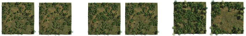

163:6 • Hädrich, T. et al.

 by the force ∈ R3 . Moreover, trees are influencing the wind which
 is captured using a drag force
 air 
 = ∥ ∥ 2 (15)
 2 ∥ ∥
 with drag coefficient and cross sectional area . All other exter-
 nal forces are combined and described by an additional external net
 force ∈ R3 . Please note that the wind speed := ∥ ∥ influences
 the reaction rate of the combustion process directly as stated in
 Eq. (2–3).

 4.4 Smoke
 We take smoke into account according to Pirk et al. [2017] who
 added smoke proportionally to the mass loss and the evaporation
Fig. 4. Illustration of the representation of a module M by an arbores- of water. Defining a time-dependent scalar field
cence M = ( , ) with nodes = { (0) , (1) , (2) , (3) , (4) }, edges
 : ( , ) ↦→ ( , )
 = { (1) := ( (0) , (1) ), (2) := ( (1) , (2) ), (3) := ( (1) , (3) ), (4) :=
( (0) , (4) ) }, and root node (0) . Node features { (0) , (1) , (2) , (3) , (4) } describing the smoke density ∈ R3 at given time ∈ R ≥0 and
and edge features { ( (1) , (1) ), ( (2) , (2) ), ( (3) , (3) ), ( (4) , (4) ) } are position ∈ R3 , its temporal evolution can be described by
shown. The unique path ( (3) ) := ( (1) , (3) ) from the root node (0) d d 
to (3) is highlighted here as an example. The depth-first search order is + · ∇ = − − (16)
 d d 
used for node numbering.
 with smoke parameters and . Pirk et al. [2017] computed the
 value of the water content by d /d = − M applying an
4.2.2 Connection Node Handling. As trees are represented by sev- evaporation rate . This is problematic because too much water
eral modules attached to each other, we distinguish between internal could also get released if the module is not burning at all. Only
and connection nodes within a module. Connection nodes are those burning wood significantly releases water vapor into the air when
which are shared by different modules (Figure 2). All other nodes the hydrogen content of the wood binds with atmospheric oxygen.
are labeled as internal nodes. For connection nodes, we store multi- With a hydrogen mass fraction in wood of 6% [Côté 1968], =
ple radii information, i.e., every module sharing a connection node, 0.5362 kg of water are released per 1 kg of burned wood when two
stores its own radius at the connection node and updates it only moles of hydrogen bind with a mole of oxygen. Consequently, we
with respect to its own mass loss rate Δ independently from the make use of the relation
other modules. However, for rendering a single radius is needed at d d 
 = . (17)
each node. For this, we simply use the average radii for connection d d 
nodes.
 4.5 Clouds and Rain
4.2.3 Charring Effect. The char insulating parameter has to be
set proportional to the char layer thickness according to Pirk et Next to the smoke density , we define similar time-dependent
al. [2017]. The char layer thickness is assumed to be the same for scalar fields for water vapor : ( , ) ↦→ ( , ), condensed water
all branches within the module. : ( , ) ↦→ ( , ), and rain : ( , ) ↦→ ( , ), which for
 given time ∈ R ≥0 and position ∈ R3 return the corresponding
4.3 Wind densities. The outputs are dimensionless quantities which we obtain
Wind is described as a time-dependent vector-valued velocity field as mass mixing ratios ([ ] = 1 kg/kg) describing the mass of vapor,
 smoke, or liquid per unit mass of air. Please note that corresponds
 : ( , ) ↦→ ( , ) to what we usually observe as visible clouds. Following Hädrich et
which for given time ∈ R ≥0 and position ∈ R3 returns the al. [2020], we model the relationship between , , and using
corresponding local flow ( , ) ∈ R3 . The temporal evolution of Kessler’s methodology [1969] including a transport equation for a
is described by the Navier-Stokes equation [Bridson 2008] rain phase in addition to vapor and cloud. The transport equations
 1 are coupled using the system of differential equations
 + · ∇ + ∇ = ∇ · ∇ + + + (13)
 air d 
 + · ∇ = − + + + − , (18)
covering the chance of momentum, and the continuity equation d 
 
 ∇· =0 (14) + · ∇ = − − − , (19)
 
ensuring the conservation of mass. In Eq. (13), the air density is 
 + · ∇ = + − − , (20)
denoted by air , the pressure by , and the kinematic viscosity by . 
The second term on the left side of Eq. (13) describes phenomena and source terms for condensation, for cloud evaporation,
caused by advection followed by the pressure term. The first term for rain evaporation, for autoconversion of raindrops from
on the right side describes viscosity. Buoyancy is taken into account clouds, and for the accretion of cloud water due to falling drops.

ACM Trans. Graph., Vol. 40, No. 4, Article 163. Publication date: August 2021.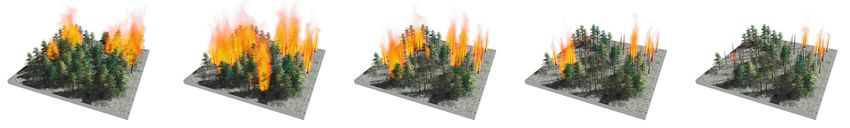

Fire in Paradise: Mesoscale Simulation of Wildfires • 163:7

 Free-slip Boundary Conditions

 Extended Kessler Model

 Wind Field Heat Transfer

 Mixed Boundary Conditions
 Mixed Boundary Conditions

 Smoke

 Module Temperature

 Radii Update Module Combustion

 Ground Elevation

 No-slip Boundary Conditions

Fig. 5. Overview of our model explicitly showing dependencies of the different quantities. The grid resolution corresponds to the size of the bounding box
of an average module. Please note that the temperature of air is used within the computations of the extended Kessler model. The outcome of the Kessler
model influences the wind field as well. Wind is furthermore directly influencing the combustion process as its reaction rate depends on the wind speed. The
combustion also depends on the updated radii as this influences the tree geometry.

We set according to Eq. (22) and add a vaporization sink term The temporal temperature change of a certain fluid parcel, as it
given by Eq. (31) as derived in the upcoming Section 4.6. Moreover, flows along the trajectory of the wind, is described by a diffusion
following Harris et al. [2003], we apply − = min( ,sat − , ), component with intensity , and an ambient cooling component
and according to Hädrich et al. [2020] = max( − , 0) and with the radiative cooling term [Nguyen et al. 2002] involving the
 = with constant , , and . Similarly to Eq. (16), fixed ambient temperature
we add a term proportional to the change of water content to
Eq. (18) in order to add the moisture released by the combustion amb := amb (ℎ) at altitude ℎ := ℎ( )
process to the water vapor. for a given position := ( , , ℎ) evaluated according to atmospheric
 data [ISO 1975]. Moreover, module to air heat transfer is addressed
4.6 Heat Transfer by adjusting the air temperature proportionally to the mass loss
The environmental temperature is described as a time-dependent with coefficient . The density of rain is taken into account to
scalar field address the cooling effect of rain. Two physical effects cause this
 cooling: Heat absorption into cool rain drops and evaporation. As
 : ( , ) ↦→ ( , ) , evaporation dominates, we will focus on this effect here. The under-
 lying physical mechanism is that water molecules leaving the rain
which for given time ∈ R ≥0 and position ∈ R3 returns the cor-
 drops have to overcome the attraction of the other water molecules,
responding environmental temperature ( , ) ∈ R. Heat transfer
 and thus cause a decrease in temperature. The driving potential of
is modeled using the following relationship describing the temporal
 this evaporation process is the relative humidity rel = / ,sat as
evolution of the air temperature :
 the ratio of the local vapor mass ratio and and the local saturation
 d vapor mass ratio ,sat [Hädrich et al. 2020] of the surrounding air.
 + · ∇ = ∇2 − ( − amb ) 4 − − . (21) When the air is saturated, i.e. = ,sat or rel = 1, evaporation
 d 

 ACM Trans. Graph., Vol. 40, No. 4, Article 163. Publication date: August 2021.

163:8 • Hädrich, T. et al.

stops and no cooling occurs. This results in a rain evaporation rate Another effect of this heat conduction is that the rain phase is
 in the form vaporized with a mass rate of ¤ = / ¤ until all rain in contact
 with the module is consumed and turned into vapor. This results in
 = max( ,sat − , 0) , (22)
 a rain vaporization sink term
where is an evaporation rate coefficient, and the saturation vapor
 ¤
  
mixing ratio is given by = max air, 0 (31)
   
 380.16 17.67 
 ,sat ( , ) = exp (23) in the presence of a tree, which has to be added to the vapor ra-
 + 243.50
 tio’s transport Eq. (18) and subtracted from the rain ratio’s trans-
for given temperature and pressure in Celsius respectively Pas- port Eq. (20).
cal [Yau and Rogers 1996]. The evaporation adsorbs the latent heat In summary, our heat model transports a temperature field, thus
 which acts to cool the surrounding air of heat capacity , such accounting for convective heat transfer including heat transfer be-
that we find an approximate expression for of Eq. (21): tween modules and the atmosphere. Radiative cooling is taken into
 account [Nguyen et al. 2002] while radiative heating is not included
 = = max( ,sat − , 0) . (24)
 as recent research [Finney et al. 2015] finds that it can be neglected
 Next to the environmental temperature field , we introduce a compared to convective heat transfer.
module temperature function
 5 ALGORITHMICS
 F : (M, ) ↦→ F (M, ) =: M ( ) , The model described in the previous section provides the basis of
which for given time ∈ R ≥0 and module M ∈ F returns the our simulator. The whole procedure is summarized in Algorithm 1.
module’s surface temperature M ( ) ∈ R. The change of M is Moreover, Figure 5 presents an overview pointing out the depen-
described by simulating diffusion between adjacent modules, as dencies of the different quantities.
well as the heating (e.g., caused by a fire) or cooling of its surface
due to the temperature of the surrounding air: ALGORITHM 1: Overview of our simulator’s numerical procedure.
 ∗ Please note that 
 M M can be precomputed for all M ∈ F.
 = M ∇2 M + ( − M ) . (25)
 Input: Current system state.
Diffusion and temperature coefficients M and are applied. More- Output: Updated system state.
 1 for each module M ∈ F do
over, we model cooling of the module’s surface due to rain, which
 2 | Update mass := ( M) according to Eq. (1).
depends on the heat transfer from the surface of the wood to the
 3 | Perform radii update according to Eq. (11–12) .
 ∗
covering water film and on the amount of rain. The heat flux to
 4 | Update temperature M according to Eq. (30).
water per unit area can be approximated by
 5 | Update released water content := ( M) according to Eq. (17).
 ¤ ′′ = ¯( M − sat ) 3 (26) 6 end

using ¯ = 0.1 Wm−2◦ C−1 and the saturation temperature of water 7 for each grid point ∈ D (Ω) do

corresponding to sat = 100◦ C [Carey 1992]. This energy is extracted 8 | Update := ( ) and := ( ) as described in Section 5.1.

from the module and added to the adjacent rain water phase until 9 end

all of the rain water is vaporized to . As an effect of this, the 10 Update temperature according to Eq. (21).

wood’s temperature is decreased. The energy M stored in a module 11 Update drag forces according to Eq. (15).

M of volume M and density M with specific heat capacity M 12 Update , , , , and according to Hädrich et al. [2020]

is given by including vorticity confinement with intensity .
 ′ 13 for each module M ∈ F do
 M = M M M M , (27)
 14 | if := ( M) = 0 then F ← F \ ( {M } ∪ children( M))
where M ′ denotes the absolute temperature. For wood, we apply
 15 end
 M ≈ 2.5 kJ ◦ C−1 kg. The temperature rate of change of the module
given a change in energy is then described by
 d M d M 1
 = , (28) 5.1 Numerical Procedure
 d d M M M
 We have to distinguish between those computations acting within
where the change in energy occurs through heat transfer across the the module space F , and those carried out on a grid discretizing our
module surface M , i.e. spatial domain Ω ⊂ R3 . As before, we denote modules as M ∈ F ,
 d M and set up a set of grid points denoted as D (Ω) discretizing Ω. We
 = ¤ ′′ M = ¤ = ¯ M ( M − sat ) 3 . (29)
 d apply a single uniform grid scale of Δ . We allow for non-flat ground
Based on this, we then extend Eq. (25) to terrains for which reason a height map H : ( , ) ↦→ H ( , ) is
 introduced defining the lower boundary of Ω:
 M ¯ M ( M − sat ) 3
 = M ∇2 M + ( − M ) − (30)
 Ωbottom := {( , , H ( , )) T ∈ Ω} .
 .
 M M M

ACM Trans. Graph., Vol. 40, No. 4, Article 163. Publication date: August 2021.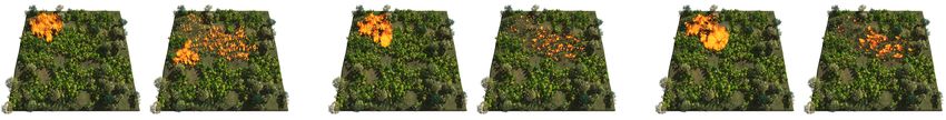

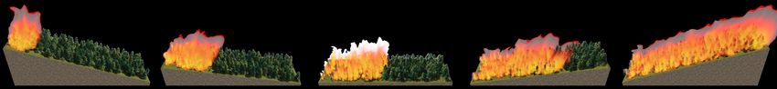
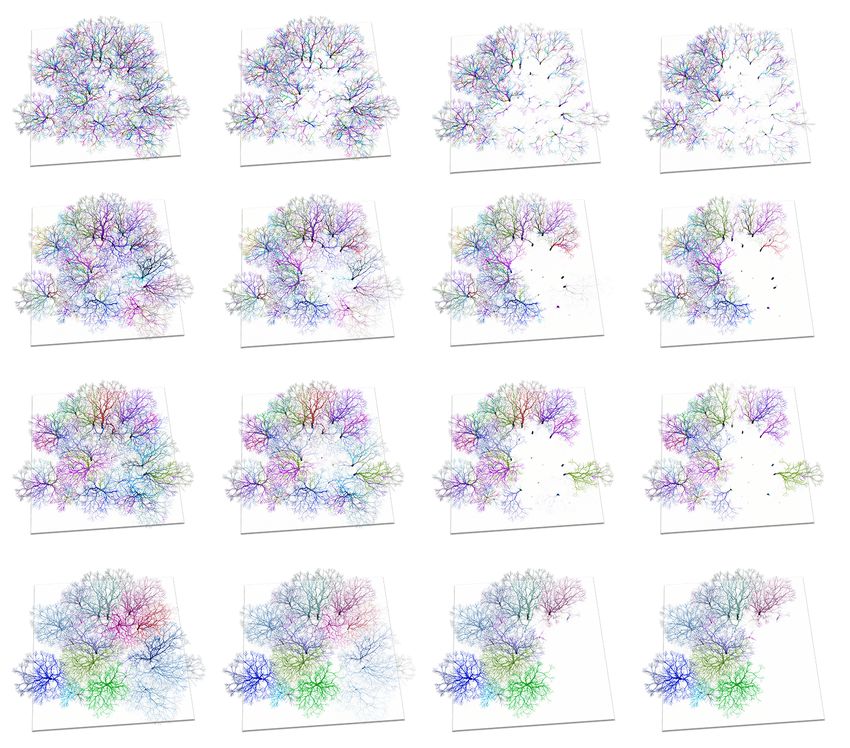
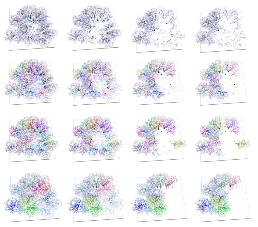
Fire in Paradise: Mesoscale Simulation of Wildfires • 163:9

Table 1. Overview of the different scenes presented in this paper. For each
scene, the spatial resolution measured in meters, the number of trees
and the number := | F | of modules, the computation time (CT) per
forward integration in milliseconds, and the relevant parameters are listed.
Each forward integration is carried out using a constant time step size of
Δ = 0.016 s. The parameters are listed in [Δ ] = 1 m, [ ] = 1 s−1◦ C−3 ,
[ ] = 1 ◦ C kg−1 , and [ ] = 1 s−1 . Identical parameters ref = 15 m/s,
 max = 2 kg s−1 m−2 , = 0.02 m2 s−1 , M = 0.75 m2 s−1 , = 1.2, =
 = 0.05 kg−1 , and = 0.2 are used throughout our simulations. The
density wood of wood (averaged for different moisture intensities) depends
on the specific tree type: deciduous = 660 kg m−3 (birches and oak trees),
 conifer = 420 kg m−3 (pine trees and spruces), and shrub = 300 kg m−3 have
been applied.

 Figure Scene Resolution Δ CT 
 1 Burning Yosemite 1603 25.0 68K 75K 82 0.003 200 1.83
 6 Vertical Spread 642 × 48 0.25 2 0.8K 2 0.003 163 0.75
 8 Varying Slope 112 × 64 × 128 2.00 3.4K 12.2K 16 0.003 163 0.75
 10 Fire Resistance 1603 2.00 19.6K 25.7K 75 0.004 200 1.83
 13 Wind Effect 1603 1.75 19.6K 25.7K 75 0.004 200 1.83
 14 Forest Cover 1603 1.75 ≤19.6K ≤25.7K ≤75 0.004 200 1.83
 15 Fire Extinguishing 642 × 48 1.00 78 5K 4 0.003 163 0.75
 15
 18
 Fire Barrier Zones
 Flammagenitus
 112 × 64 × 128
 128 × 24 × 92
 2.00
 10
 ≤3.4K
 1K
 ≤12.2K
 2.5K
 ≤13
 6
 0.003
 0.003
 163
 163
 0.75
 0.75
 Fig. 7. Analysis of the effect of different numbers of modules by studying a
 19 Flammagenitus 1603 25.0 120K 120K 95 0.003 200 1.83 small ecosystem (left) and an individual tree (right). The average number of
 modules per tree within the ecosystem (left) is given by 55, 7, 5, and 1 (from
 top to bottom). The single tree (right) is decomposed into 123, 68, 19, 14
 modules, and into a single module (from top to bottom). The corresponding
 mass loss is shown in the diagrams below.

 which return mass ( ) := ( , ) and water content ( ) :=
 ( , ) relative to a grid point (i.e. cell center point) ∈ D (Ω) for
 a fixed point in time ∈ R ≥0 . These quantities are computed by
 taking into account all modules M which (partially) overlap with
 the cell around , summing up their masses or water content
 weighted by a factor of (1 − ∥ − center(M)∥/Δ ) in which
 center(M) denotes the center of mass of M. Based on this, temper-
 atures can be updated according to Eq. (21) as well as , , , ,
 and according to the Eulerian fluid solver of Hädrich et al. [2020].
 Here, we include drag forces according to Eq. (15) into the exter-
 nal forces in Eq. (13). We apply no-slip boundary conditions at the
 Fig. 6. Vertical fire spread onto a big tree from a small tree underneath. ground, free-slip conditions conditions at the top, and mixed bound-
 ary conditions at the sides [Hädrich et al. 2020]. Moreover, vorticity
 confinement is included as nonphysical damping caused by numeri-
 The procedure summarized in Algorithm 1 starts with an itera- cal dissipation removes interesting turbulent flow features. To avoid
tion over all modules M ∈ F updating their masses according to this, a vorticity confinement force as introduced by Steinhoff and
Eq. (1). For this, reaction rates have to be computed according to Underhill [1994] is applied, which injects the dissipated energy back
Eq. (2) for a given module temperature using a threshold velocity of into the system. The strength of the vorticity confinement can be
 ref = 15 m/s corresponding to strong wind boosting the reaction adjusted using a parameter according to Fedkiw et al. [2001].
rate by a factor of max . The local velocity of = ∥ ∥ is computed Finally, we check which modules M completely burned down
as the average absolute wind speed within the cells which contain (a (i.e. (M) = 0) and remove them from the module space F as well
part of) the corresponding module. The mass updates are followed as their children within the arborescence.
by radii updates according to Eq. (11–12). Then, module tempera-
 5.2 Implementation
tures M are computed according to Eq. (30), and released water
contents are estimated according to Eq. (17). We implemented Algorithm 1 within a C++/CUDA framework.
 Please note that mass = (M) and water content = (M) When updating mass, water content, and temperatures, we employ
are computed per module and have to be transferred to the grid regular forward finite differences. Moreover, Hädrich et al. [2020]
in order to update temperature (Eq. (21)) and water vapor density kindly provided the source code of their cloud simulator, which we
(Eq. (18)), and to simulate smoke (Eq. (16)). Consequently, we intro- extended by including an additional term proportional to the change
duce time-dependent scalar fields of water content to Eq. (18) as well as our novel formulations for
 given by Eq. (22) and given by Eq. (31). Please note that their
 : ( , ) ↦→ ( , ) and : ( , ) ↦→ ( , ) , implementation utilises the concept of potential temperature, hence

 ACM Trans. Graph., Vol. 40, No. 4, Article 163. Publication date: August 2021.

163:10 • Hädrich, T. et al.

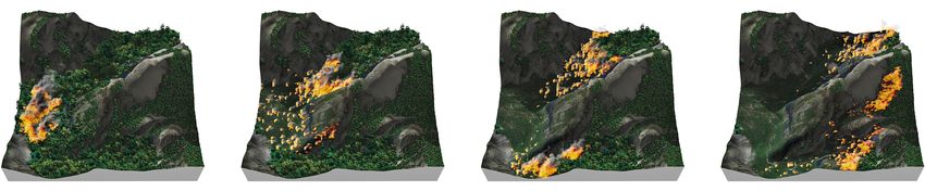
 Fig. 8. Snapshots showing simulations of fire spread on inclined planes with different slope angles ∈ {−20◦ , −10◦ , 0◦ , 10◦ , 20◦ } (from left to right).

we have to convert our absolute temperature values to potential We evaluate our module-based representation by comparing sim-
temperature and vice versa when using their solver. ulation results using different numbers of modules. As shown in
 For rendering purposes, volume ray casting [Pharr et al. 2016] Figure 7 (top), we provide a qualitative comparison by simulating an
is employed using OpenGL/GLSL evaluating rays of light as they individual tree as well as an ecosystem. A quantitative comparison
pass through the volume. Tree geometries and leaves are handled is given in Figure 7 (bottom) monitoring the mass loss over time for
dynamically in the geometry shader. For each pixel intersecting different numbers of modules.
the volume, opacity and color are returned and visualized on the
screen in real-time, which allows for the interactive exploration of 6.3 Coarse-scale Comparison
our simulations.
 To showcase the impact of taking detailed branch geometry into
6 RESULTS account, we simulate fire spread within an ecosystem composed of
 several conifers arranged on a flat terrain. As shown in Figure 9,
We present an overview of our results simulated according to Algo-
 the fire spread is simulated with our mesoscale approach as well
rithm 1 implemented as described in the previous section. Initial tree
 as by using a simplified coarse-scale representation which mimics
geometries were generated using the ecosystem simulator developed
 certain properties of the ecosystem on a higher level of abstraction.
by Makowski et al. [2019], who kindly provided their software. An
 Each tree is represented as a single cylindrically shaped trunk whose
overview of the different scenes presented throughout this section
 mass corresponds to the mass of the whole tree in the mesoscale rep-
is provided in Table 1 including relevant parameters. The scenes can
 resentation. In particular, the wood density is adopted, the trunk’s
be simulated interactively or even in real-time. The computation
 height corresponds to the height of the tree in the mesoscale rep-
times listed in Table 1 are measured on an up-to-date desktop com-
 resentation, and the trunk’s diameter is adjusted in a way that the
puter running our simulation framework on an NVIDIA® GeForce
® GTX 1080. trunk’s mass equals the sum of the tree’s module masses. While
 using the mesoscale approach, some time is required until a single
 tree potentially burns completely, the coarse-scale representation
6.1 Fire Spread results in a direct inflammation of the whole trunk which immediate
The use of detailed branch geometry allows us to realistically capture starts to burn brightly as detailed branch geometry is not considered.
the three-dimensional fire spread, which cannot be easily covered As we mimic the original tree widths, the fire propagates remark-
with other representations or statistical models. For example, when ably fast through the ecosystem resulting in an unrealistic wildfire
a tree underneath another tree is burning, fire can spread vertically scenario. This is quantitatively evaluated in Figure 11 (right) which
as illustrated in Figure 6. This would not occur in simplified spatial shows the relative change of mass within the whole ecosystem. It
representations such as statistical models. We further demonstrate can be observed that the coarse-scale representation results in a fast
the effect of fire spread in a forest using a constant horizontal wind combustion of a major part of the ecosystem while the mesoscale
field. We vary the slope of the ground terrain. As expected, for approach leads to a distinctively different result.
a positive slope the fire spreads faster compared to a flat terrain
or a negative slope. This is qualitatively illustrated in Figure 8 and 6.4 Ecosystem Properties
quantitatively evaluated in Figure 11 (left), indicating an exponential
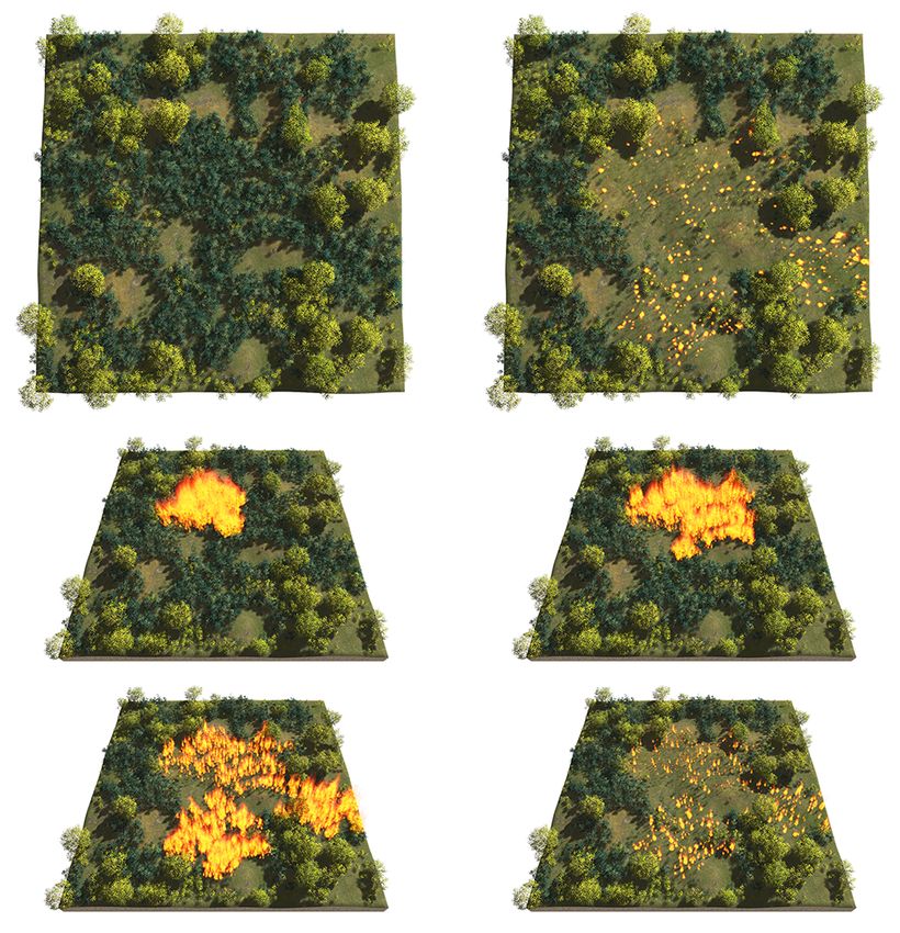
 Our framework allows for studying the influence of different ecosys-
decrease of the propagation time with increasing slope.
 tem properties. First, we investigate the impact of different tree types
 as illustrated in Figure 10. In particular, we simulate the temporal
6.2 Mesoscale Representation evolution of a wildfire within an ecosystem which contains conifers
The mesoscale representation for trees enables us to model collec- and deciduous trees. We observe that the deciduous trees are more
tions of trees with detailed branch geometry for individual modules. fire resistant compared to the conifers, which is partially caused by
Specifically, modeling trees with modules enables controlling the their higher density. This results in a characteristic change of the
level of detail. Neither coarse-scale nor fine-scale representations forest pattern caused by the wildfire, changing the ratio of conifers
offer these two benefits at once. Furthermore, trees dynamically and deciduous trees within the ecosystem.
adapt to their individual environment, which cannot simply be rep- Moreover, we study the impact of the forest cover (i.e. the relative
resented by fixed proxy shapes such as cones. Modules capture both amount of land covered by trees) on the wildfire. As reported in the
the self-organization as well as the recursive attribute of tree archi- literature [Abades et al. 2014], we observe that below a specific forest
tecture, thus leading to a more realistic geometric representation. coverage, fire spread is inhibited as there is not sufficient biomass to

ACM Trans. Graph., Vol. 40, No. 4, Article 163. Publication date: August 2021.

Fire in Paradise: Mesoscale Simulation of Wildfires • 163:11

 Fig. 11. Left: Dependence of the speed of the fire spread on different slope
 values indicating an exponential trend. For an angle of −20◦ the fire extin-
 guished itself, not being able to propagate over the whole negatively sloped
 plane. Right: Temporal evolution of the mass (relative to the initial mass)
 measured from the simulation using our detailed mesoscale approach (blue)
Fig. 9. Temporal evolution (from left to right) of a wildfire burning down and by using a simplified coarse-scale model (orange).
conifers simulated with our detailed mesoscale approach (top) and by using
a simplified coarse-scale model (bottom). The mesoscale representation
contains on average 85 modules per tree. As shown in the left images, the
complete left tree front is initially set on fire.

 Fig. 12. Left: Dependence of the relative number of trees with burned mod-
 ules on the forest coverage. Once a threshold of about 58% of forest cover is
 reached, the fire is spreads over the whole ecosystem. Right: Cohort of trees
 are cut resulting in empty fire barrier zones of different widths. The number
 of trees with burned modules depending on the width is shown here.

 Fig. 13. Left: Temporal evolution of the relative number of burned trees for
 different scenarios without wind (blue), with moderate wind (orange), and
 with strong wind (red). Right: Equivalent results predicted by a percolation
Fig. 10. Temporal evolution (middle and bottom row) of a wildfire burning
 model expressing the effects of wind on fire spread for the same vegetation
down conifers and deciduous trees. The fact that the deciduous trees are
 scene. Both models predict a decrease in burned tree ratios with increasing
more fire resistant compared to the conifers results in a different forest
 wind speed. The handling of the percolation model is described by Abades
pattern (top right) compared to the state before the wildfire (top left).
 et al. [2014] who kindly provided their source code.

propagate the fire. In contrast, once a specific threshold is reached,
the fire spreads intensively. The graph in Figure 12 (left) shows the in Figure 12 (right) is expected as flying sparks are ignored in our
relative number of trees with burned modules for different forest model.
cover. The corresponding ecosystems are shown in Figure 14.
 6.6 Atmospheric Conditions
6.5 Wildfire Management We study the impact of different atmospheric conditions by varying
Modern wildfire management comprises fire prevention and re- the speed of a constant horizontal wind field as shown in Figure 17.
sponse as well as recovery work. To evaluate the human impact This is quantitatively evaluated in Figure 13 showing the relative
on wildfires, our model allows us to interactively extinguish fire number of burning trees (including already burned trees) over time.
by manually distributing fire retardant as well as by setting up fire As expected, the fire spreads faster with increasing wind speed,
barriers. This is qualitatively illustrated in Figure 15. Moreover, we which is caused by the propagation of flames due to wind as well as
quantitatively evaluate the impact of fire barriers using different the fact that fire increases its temperature and accelerates the com-
barrier widths as shown in Figure 12 (right). Once a specific thresh- bustion process if wind is blowing oxygen into the fire (see Eq. (3)).
old width of about 7.9 m in our example is reached, the fire is not Consequently, the relative number of burned trees increases faster
able to jump over the barrier. Please note that the discrete jump in the beginning of the wildfire when wind is stronger. However, as

 ACM Trans. Graph., Vol. 40, No. 4, Article 163. Publication date: August 2021.

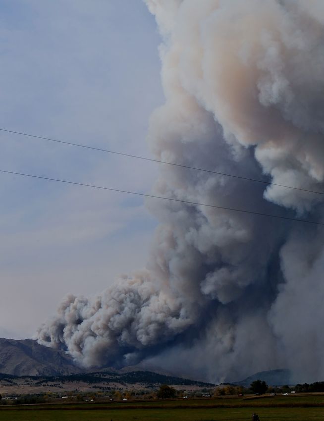
163:12 • Hädrich, T. et al.

 Fig. 14. Illustration of the fire spread in different ecosystems varying with respect to their initial forest cover of 25% (left), 45% (middle), and 90% (right).

Fig. 15. Top: Illustration of the user experience of our interactive wildfire simulator. Simulation and rendering are running in real-time so that the user can
conveniently explore the scene. After inspecting the wildfire, fire retardant is interactively distributed partially extinguishing the fire. The application of fire
retardant is implemented by setting the module temperature to the environmental temperature at selected trees. Bottom: The temporal evolution of a scenario
is shown in which the user sets up an empty fire barrier zone by cutting trees. As the width of the barrier zone is not sufficient to protect the forest, the fire
spreads over the zone further increasing forest damage.

it can be observed from Figure 13 as well, wind also blows the fire in thunderstorms from which lightning can become an additional fire
a dominant direction, potentially hindering it to spread isotropically, source [Dowdy et al. 2017]. Figure 18 shows the simulation of a
resulting is less forest damage in the long-term. wildfire scenario from which a flammagenitus cloud emerges whose
 rainfall finally extinguishes the fire. The scene is rendered from a
6.7 National Park Wildfire cross-sectional perspective highlighting water vapor and condensed
 cloud water showcasing the formation of the flammagenitus cloud.
We simulate a complex wildfire originating from a randomly po-
 A more complex scene comprising a huge flammagenitus cloud
sitioned fire source which could be caused by a lightning strike.
 over a wildfire is shown in Figure 19. This scene comprises 120K
The fire spreads within the valley around Half Dome in California’s
 individual trees grown on a mountainous terrain. It runs at interac-
Yosemite National Park as shown in Figure 1. This scene contains
 tive rates. As a comparison, a photography of a real flammagenitus
about 68K trees composed of about 75K individual modules. The
 cloud is shown in Figure 16. While dark smoke is present at lower
simulation runs at interactive rates.
 altitudes, the condensation of water at higher altitudes results in a
 white cumuliform cloud. This can be observed in our simulation as
6.8 Flammagenitus Clouds well as in the photography.
 Flammagenitus clouds are dense grayish
 to brown cumuliform clouds which po- 7 DISCUSSION
 tentially emerge from wildfires or vol- An important result of analytical studies on forest fires (e.g. using
 canic eruptions. While it may seem coun- percolation models) is that the geometric distribution of vegetation
 terintuitive that water vapor condenses in space is a major determinant of fire spread. Consequently, the
 to form clouds in the vicinity of a hot predictive power of wildfire simulators depends on detailed tree
 flame, Eq. (17) reveals that burning wood form representations. Existing theoretical methods study wildfires
 releases large amounts of water that su- by employing coarse tree representations, such as 2D grids, voxels or
 persaturate the air above a fire. The ef- cones [Mendoza et al. 2019]. In contrast, our method proposes a sig-
 fect of flammagenitus clouds on wildfires nificantly more detailed representation of tree form based on branch
 is two-fold and dependent on the size modules. Our comparison to a coarse-scale model (Section 6.3) show-
Fig. 16. Photography and intensity of the fire. Flammagenitus cases the importance of detailed tree geometry.
of a flammagenitus. clouds can condense, resulting in rainfall Our simulation results indicate that wildfires are characterized
 contributing to potentially extinguishing by a tipping-point phenomenon. Specifically, we report that with
the fire. On the other hand, huge wildfires can produce growing flam- increasing forest cover the burned tree ratio increases following a
magenitus clouds (cumulonimbus flammagenitus) which can trigger hill-shaped relation (Figure 12, left). Such a non-linear relation is

ACM Trans. Graph., Vol. 40, No. 4, Article 163. Publication date: August 2021.