Ergodic Edge Modes in the 4D Quantum Hall Effect
←
→
Page content transcription
If your browser does not render page correctly, please read the page content below
Ergodic Edge Modes in the 4D Quantum Hall Effect

                                                           Benoit Estienne, Blagoje Oblak, ♠ and Jean-Marie StéphanF
                                                    estienne@lpthe.jussieu.fr, boblak@lpthe.jussieu.fr, stephan@math.univ-lyon1.fr

                                                                  Sorbonne Université, CNRS, Laboratoire de Physique Théorique
                                                                       et Hautes Énergies, LPTHE, F-75005 Paris, France;
arXiv:2104.01860v1 [cond-mat.mes-hall] 5 Apr 2021

                                                                   ♠ Centre de Physique Théorique, CNRS, Ecole Polytechnique,

                                                                               UMR 7644, F-91128 Palaiseau, France;
                                                              F   Univ Lyon, CNRS, Université Claude Bernard Lyon 1, UMR 5208,
                                                                      Institut Camille Jordan, F-69622 Villeurbanne, France.

                                                                                           Abstract
                                                      The gapless modes on the edge of four-dimensional (4D) quantum Hall droplets
                                                      are known to be anisotropic: they only propagate in one direction, foliating the 3D
                                                      boundary into independent 1D conduction channels. This foliation is extremely
                                                      sensitive to the confining potential and generically yields chaotic flows. Here
                                                      we study the quantum correlations and entanglement of such edge modes in 4D
                                                      droplets confined by harmonic traps, whose boundary is a squashed three-sphere.
                                                      Commensurable trapping frequencies lead to periodic trajectories of electronic
                                                      guiding centers; the corresponding edge modes propagate independently along S 1
                                                      fibers, forming a bundle of 1D conformal field theories over a 2D base space. By
                                                      contrast, incommensurable frequencies produce quasi-periodic, ergodic trajecto-
                                                      ries, each of which covers its invariant torus densely; the corresponding correlation
                                                      function of edge modes has fractal features. This wealth of behaviors highlights
                                                      the sharp differences between 4D Hall droplets and their 2D peers; it also exhibits
                                                      the dependence of 4D edge modes on the choice of trap, suggesting the existence
                                                      of observable bifurcations due to droplet deformations.

                                                                                               1
Contents
1 Introduction . . . . . . . . . . . . . . . . . . . . . . . . . . . . . . . . . . . .                                                           3

2 Classical edge dynamics . . . . . . . . . . . . . . . . . . . . . . . . . . . . .                                                              5
  Guiding center approximation . . . . . . . . . . . . . . . . . . . . . . . . . . .                                                             5
  Harmonic potential in 4D . . . . . . . . . . . . . . . . . . . . . . . . . . . . .                                                             6

3 Quantum correlations . . .         .   .   .   .   .   .   .   .   .   .   .   .   .   .   .   .   .   .   .   .   .   .   .   .   .   .   .    7
  One-body spectrum . . . . . .      .   .   .   .   .   .   .   .   .   .   .   .   .   .   .   .   .   .   .   .   .   .   .   .   .   .   .    8
  Isotropic droplets . . . . . . .   .   .   .   .   .   .   .   .   .   .   .   .   .   .   .   .   .   .   .   .   .   .   .   .   .   .   .    9
  Rational anisotropic droplets .    .   .   .   .   .   .   .   .   .   .   .   .   .   .   .   .   .   .   .   .   .   .   .   .   .   .   .   11

4 Ergodic edge modes . . . . . . . . . . . . . . . . . . . . . . . . . . . . . . .                                                               13
  Continued fractions and numerics . . . . . . . . . . . . . . . . . . . . . . . . .                                                             13
  Fractal correlations . . . . . . . . . . . . . . . . . . . . . . . . . . . . . . . . .                                                         14

5 Quantum entanglement . . . . . . . . . . . . . . . . . . . . . . . . . . . . .                                                                 17
  Spherical cap and area law . . . . . . . . . . . . . . . . . . . . . . . . . . . . .                                                           18
  Gapless entanglement on an interval . . . . . . . . . . . . . . . . . . . . . . .                                                              20

6 Conclusion and outlook . . . . . . . . . . . . . . . . . . . . . . . . . . . . .                                                               22

A One-body dynamics in a harmonic trap . . . . . . . . . . . . . . . . . . . .                                                                   24
  Classical dynamics; guiding center approximation . . . . . . . . . . . . . . . .                                                               24
  Quantum dynamics; LLL projection . . . . . . . . . . . . . . . . . . . . . . . .                                                               24

B Asymptotics of the incomplete gamma function                                       .   .   .   .   .   .   .   .   .   .   .   .   .   .   .   25
  (i) Stationary phase paths . . . . . . . . . . . . . .                             .   .   .   .   .   .   .   .   .   .   .   .   .   .   .   25
  (ii) Integration contours . . . . . . . . . . . . . . .                            .   .   .   .   .   .   .   .   .   .   .   .   .   .   .   26
  (iii) Evaluating asymptotics . . . . . . . . . . . . .                             .   .   .   .   .   .   .   .   .   .   .   .   .   .   .   28

C Edge correlations in anisotropic droplets                          .   .   .   .   .   .   .   .   .   .   .   .   .   .   .   .   .   .   .   29
  (i) Method of images . . . . . . . . . . . . .                     .   .   .   .   .   .   .   .   .   .   .   .   .   .   .   .   .   .   .   29
  (ii) Individual asymptotics . . . . . . . . .                      .   .   .   .   .   .   .   .   .   .   .   .   .   .   .   .   .   .   .   30
  (iii) Series approximation . . . . . . . . . .                     .   .   .   .   .   .   .   .   .   .   .   .   .   .   .   .   .   .   .   30

D Entanglement in a spherical        cap         .   .   .   .   .   .   .   .   .   .   .   .   .   .   .   .   .   .   .   .   .   .   .   .   32
  (i) Overlap asymptotics . . .      . . .       .   .   .   .   .   .   .   .   .   .   .   .   .   .   .   .   .   .   .   .   .   .   .   .   32
  (ii) Leading entanglement . .      . . .       .   .   .   .   .   .   .   .   .   .   .   .   .   .   .   .   .   .   .   .   .   .   .   .   33
  (iii) Subleading entanglement      . . .       .   .   .   .   .   .   .   .   .   .   .   .   .   .   .   .   .   .   .   .   .   .   .   .   34

References . . . . . . . . . . . . . . . . . . . . . . . . . . . . . . . . . . . . . . .                                                         35

                                                         2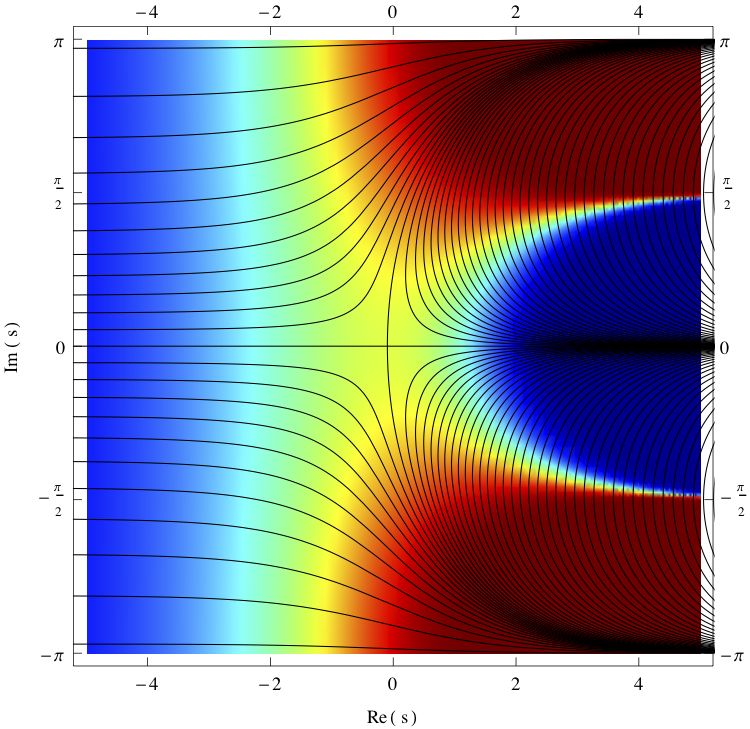
1         Introduction
 Spurred by the discovery of the quantum Hall effect (QHE) [1,2], the study of topological
 phases has been one of the driving forces of condensed matter physics in recent decades
 [3, 4]. By now, numerous such topological systems have indeed been found, both in
 genuine condensed matter [5–7] and in its various simulations [8–13]. The latter offer the
 exciting prospect of realizing exotic phases that do not, otherwise, occur spontaneously
 in Nature. One such exotic system is the QHE in dimensions higher than two.
    Theoretical aspects of higher-dimensional Hall droplets have been investigated ever
 since the proposal of [14], where electrons on a four-sphere were subjected to a non-
 Abelian background gauge field. It was quickly noticed, however, that the interesting
 phenomenology of this model — Landau levels, non-commutative space, non-trivial bulk
 topological invariants and chiral edge modes — also occurs in 4D systems that simply
 support an Abelian magnetic field [15–20], readily generalizing the 2D QHE. (In partic-
 ular, as in 2D, the symplectic interpretation of non-commutative geometry [21–23] then
 connects quantum Hall physics to geometric quantization [24–28].)
    A staple of these works is the anisotropic nature of edge modes [15–17]: while low-
 energy excitations of a 2D droplet propagate along the entire 1D boundary, their higher-
 dimensional peers are localized on 1D fibers embedded in a higher-dimensional manifold.
 The gapless edge modes of a 4D droplet thus span a collection of (1+1)-dimensional chiral
 conformal field theories (CFTs), rather than a (3+1) CFT. As a result, edge dynamics
 is exceedingly sensitive to the trapping potential: it can range from fully integrable to
 chaotic, depending on the trap. The present paper is therefore devoted to a detailed
 analysis of such boundary excitations in a microscopic model of trapped 4D ‘electrons’
 in a strong magnetic field.1 Since we shall rely on quantum-mechanical methods similar
 to those used to describe ultracold atoms [8–11] and topological photonics [12, 13], our
 hope is also to provide a bridge between field-theoretic considerations [15–20] and the
 vast literature on synthetic dimensions [29–38].
   For definiteness we will focus on harmonic traps, where electron dynamics is integrable
 and the boundary is a (squashed) 3D sphere. Electronic guiding center orbits are then
 localized on invariant 2D tori and can be either periodic or quasi-periodic. In particular,
 edge modes of isotropic droplets realize the Hopf fibration of S 3 (see fig. 1), while edge
 modes in anisotropic traps are generally ergodic in the sense that each of their orbits
 covers its torus densely. These results rely on the following series of arguments:
(i) First, we shall see how some of the most striking properties of edge modes can already
    be inferred from the classical picture of skipping electrons whose guiding centers follow
    equipotentials. This will show that, at strong magnetic fields, any trapping potential
    produces 1D edge modes in an otherwise higher-dimensional boundary (see figs. 2–
    3). This fact — essentially restating the classical Hall conductance formula — readily
    implies that the global structure of edge trajectories hinges on the degree of anisotropy
    of the trap, suggesting the existence of ergodic and chaotic regimes.
(ii) We will then study quantum corrections of this classical approximation by evaluating
     the many-body ground state correlation function of a non-interacting 4D droplet. Trap-
     ping anisotropies with rational frequency ratios will allow us to evaluate the asymp-
     1
         The 4D restriction is a matter of convenience: our conclusions extend to higher-dimensional droplets.

                                                        3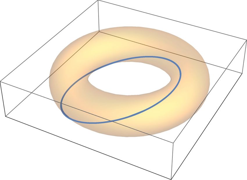
Figure 1: A portion of the Hopf fibration of S 3 (here visualized using stereographic
  projection to R3 ): each fiber is a circle S 1 labelled by a point in an S 2 base space [45].
  The trajectories of edge modes in an isotropic 4D quantum Hall droplet coincide with
  such S 1 fibers in an S 3 boundary; they are localized on nested tori, each of which is itself
  partitioned into (chiral) Villarceau circles. By contrast, in generic anisotropic droplets,
  each torus is filled densely by a single edge mode trajectory.

     totics of correlations near the boundary (see eq. (20) below). As we shall see, edge
     correlations indeed localize on classical guiding center trajectories, along which they
     satisfy a power-law characteristic of 1D CFTs, while they decay in a Gaussian manner
     in all remaining directions. This is depicted in fig. 7; note in particular the delicate
     dependence of edge correlations on the trap’s anisotropy.
(iii) The second step of our analysis of correlations will be concerned with ‘irrational’
      anisotropic traps, where the asymptotic methods appropriate for periodic edge modes
      fail to apply. Nevertheless, semiclassical intuition, supported by ample numerical evi-
      dence (see figs. 8–9), will allow us to analyse edge correlations in the thermodynamic
      limit. This is expressed in eq. (25) and plotted in fig. 10; it involves a function that
      vanishes almost everywhere but takes non-zero values on a dense subset of the torus,
      displaying fractal-like properties and a certain degree of self-similarity.
(iv) Finally, we shall estimate the ground state entanglement of various spatial regions
     crossing the edge of a 4D droplet, thus generalizing the 2D considerations of [39]. The
     derivation will rely on well established techniques relating the entanglement spectrum
     of free fermions to their correlations [40–44]. For regions whose boundary is parallel to
     edge fibers, subleading contributions to entanglement entropy will turn out to vanish,
     confirming that edge modes on distinct fibers are genuinely independent. By contrast,
     the entanglement entropy of regions that cut through certain fibers will display the
     logarithmic behavior expected of a bundle of 1D CFTs, with a total central charge
     related to the bulk Fermi energy.
  The plan of the paper follows this sequence: section 2 is classical, quantum correlations
  of periodic and ergodic edge modes are respectively studied in sections 3–4, and entangle-
  ment is treated in section 5. The back matter contains various technical details, such as
  the exact spectrum of a trapped 4D Landau Hamiltonian (appendix A) or the derivation
  of asymptotic relations needed in sections 3 (appendices B–C) and 5 (appendix D).

                                                4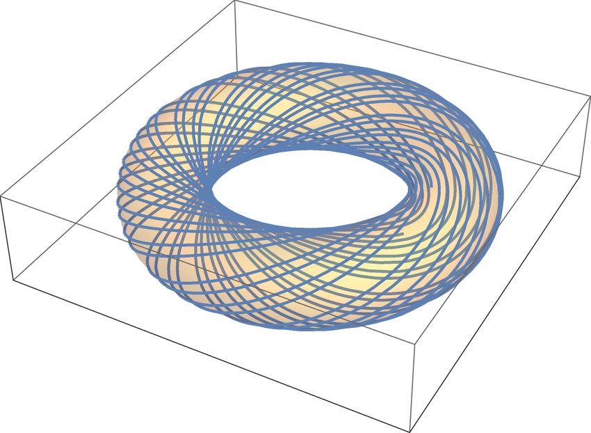
2         Classical edge dynamics
Guided by classical intuition, this section serves to develop basic expectations about
the edge modes of Hall droplets in any dimension, with arbitrary trapping potentials.
This will rely on the well-known projected form of the Landau Hamiltonian at strong
magnetic fields [46]. As an example, we introduce the harmonic 4D Landau Hamiltonian
that will be used throughout this work. Technical details regarding the spectrum of this
Hamiltonian are relegated to appendix A.

Guiding center approximation. Consider a massive charged particle in Rd (d even);
we work in natural units, so mass = charge = 1. Points in Rd are written as vectors x
with components xi , i = 1, ..., d. We assume (i) that some confining potential V (x) is
present, (ii) that the system supports a magnetic field B = dA for some vector potential
A, such that the matrix Bij (x) = ∂i Aj − ∂j Ai is invertible everywhere. At very strong
magnetic fields, kinetic energy may be neglected and the Lagrangian of the particle
reduces to L = A(x) · ẋ − V (x). This is linear in velocities, so canonical momenta are
not independent coordinates on phase space; they are, instead, related to positions:
                                                     ∂L
                                               p≡         = A(x).                                          (1)
                                                     ∂ ẋ
This equality may be seen as a set of d constraints2 p − A(x) ≈ 0 determining the
components pi from the knowledge of spatial coordinates xi . Because d is even and B is
non-degenerate, these constraints are second class and yield a Dirac bracket [47, sec. 1.3]

                                                {xi , xj } = B ij ,                                        (2)

where B ij is the inverse matrix of the magnetic field Bij . As a result, one may think of
Rd itself as a phase space with (classical) coordinates xi that fail to Poisson-commute,
the magnetic field playing the role of a symplectic form. The Hamiltonian projected on
this effective phase space coincides with the trapping potential:
                                           1
                                  H(x, p) = (p − A)2 + V (x) ≈ V (x),                                      (3)
                                           2
so that the pure Landau term (p − A)2 /2 is minimized. This approximation is a classical
analogue of the quantum projection to the lowest Landau level [46]. In particular, the
projected Hamiltonian describes the slow motion of guiding centers of cyclotron orbits:
using (3) and the bracket (2), one finds

                                         ẋi ≈ {xi , V (x)} = B ij ∂j V.                                   (4)

Our presentation of this result used the formalism of constrained systems for brevity, but
a more intuitive argument can also be provided. Indeed, the guiding center approxima-
tion stems from a separation of time scales (fast cyclotron rotations versus slow guiding
center drift) in strong magnetic fields. This splitting becomes sharper as the magnetic
field increases and cyclotron orbits with bounded energy shrink, eventually leading to
an elimination of fast degrees of freedom and a dimensional reduction to the so-called
    2
        The (standard) notation ≈ denotes equalities that hold on the constraint surface specified by (1) [47].

                                                        5
Arg(u+iv)

                                Arg(u+iv)
            Arg(x+iy)                             Arg(x+iy)

Figure 2: The motion (6) of a guiding center on a torus (at fixed x2 + y 2 and u2 + v 2 ),
initially located in the square’s lower
                                     √ left corner. From left to right, the frequency ratio
(7) takes values ∆ = 1, 5/3 and 2. The first and second cases (∆ = 1 or 5/3) are
rational, producing periodic
                        √      guiding center motion; ∆ = 1 is even isotropic. By contrast,
the third case (∆ = 2) is not only anisotropic, but irrational. As a result, even a
single guiding center trajectory covers the torus densely; the color-coding is such that the
trajectory is initially black, then progressively fades to white. These pictures should be
compared with their quantum counterparts, namely the edge correlations of figs. 7–8.

slow manifold [48]. Here, the latter is just the space Rd of guiding center positions en-
dowed with the Poisson bracket (2) and the effective Hamiltonian V (x), yielding the slow
dynamics (4).
   In 2D, the equation of motion (4) is necessarily integrable, so its implications are
somewhat trivial: guiding centers follow 1D equipotentials of V (x), merely restating the
classical Hall law (namely that the current B ij ∂j V is perpendicular to the electric field
∂j V ). The situation is much richer in higher dimensions, where periodic trajectories only
occur in highly symmetric potentials, while generic traps (with compact equipotentials)
produce ergodic, or even chaotic, guiding center dynamics. We do not investigate the
fully chaotic situation in this work. Instead, we focus on a family of integrable setups
whose edge modes lie on Liouville-Arnold tori, in which case the possibility of resonances
entails higher-dimensional subtleties that never affect 2D droplets. For instance, in 4D,
integrable guiding center motion is specified by two frequencies; rational frequency ratios
then produce periodic trajectories (fig. 1 + left and center panels of figs. 2–3), but irra-
tional ratios entail quasi-periodic, ergodic trajectories, each of which is everywhere dense
on its torus (rightmost panels of figs. 2–3). Sections 3 and 4 will respectively describe the
quantum correlations of edge modes corresponding to those two cases. For now, however,
we remain in the classical realm.

Harmonic potential in 4D. Let us illustrate the general arguments above with a simple
example to which we shall refer repeatedly. Assume d = 4 and write x = (x, y, u, v), with
a uniform magnetic field B = B(dx ∧ dy + du ∧ dv). Let the trapping potential be
harmonic and partially isotropic, with stiffnesses k, k 0 > 0:

                                            k 2           k0
                            V (x) =           (x + y 2 ) + (u2 + v 2 ).                  (5)
                                            2             2
In the slow guiding center phase space R4 with Poisson brackets (2), this trap may be
viewed as the Hamiltonian of a 2D harmonic oscillator. This is the canonical example of a

                                                    6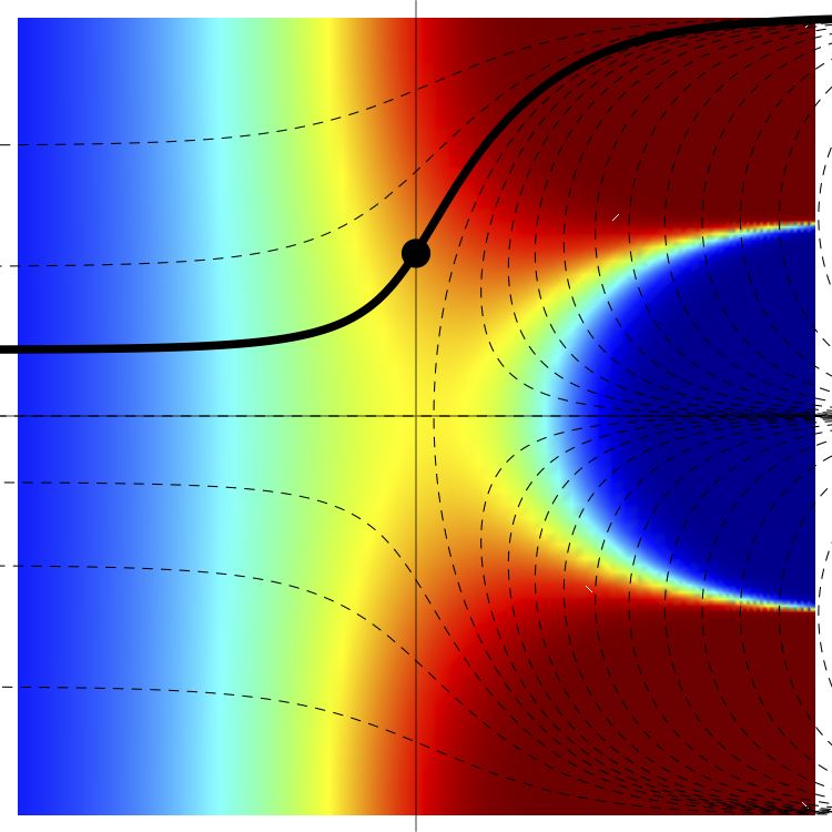
classical integrable system: one trivially has two conserved quantities (x2 +y 2 and u2 +v 2 ),
so guiding center trajectories lie on tori at constant x2 + y 2 and u2 + v 2 . Furthermore,
the ‘Hamiltonian’ (5) is quadratic, so the slow equation of motion (4) is linear:

                       ẋ = −ωy,        ẏ = ωx,         u̇ = −ω 0 v,     v̇ = ω 0 u,                   (6)

with ω ≡ k/B, ω 0 ≡ k 0 /B, both assumed to be much smaller than the cyclotron frequency
ωc = B. Guiding centers thus rotate in the (x, y) and (u, v) planes with respective
frequencies ω and ω 0 ; their winding around the torus depends on the ratio

                                               ∆ ≡ ω 0 /ω.                                              (7)

Note that the quadratic potential (5) is so simple that the dynamics of the full Hamilto-
nian H = (p − A)2 /2 + V (x) is actually integrable, even without projecting to the slow
manifold as was done here. This derivation is exposed in appendix A. Its results only
differ from those just displayed by small corrections, proportional to the (dimensionless)
parameter pk/B  1. For instance,
                2
                                     the actual ratio of guiding center frequencies on the
torus is ( 1 + 4k 0 /B 2 − 1)/( 1 + 4k/B 2 − 1), which indeed reduces to (7) at large B 2 /k.
                               p

   It is worth pausing to appreciate the different regimes that occur depending on the value
of the ratio (7). The simplest, fully isotropic setup has ∆ = 1; guiding center trajectories
then partition their S 3 equipotential into linked circles S 1 , each labelled by a point in a
Bloch sphere S 2 , producing the Hopf fibration S 1 → S 3 → S 2 (fig. 1).3 More generally,
any rational ratio (7) leads to periodic trajectories in a (squashed) S 3 , generalizing the
isotropic case so that each equipotential is a (covering of a) lens space [49], with distinct
fibers again labelled smoothly by points in S 2 . By contrast, when ∆ is irrational, the
motion of x(t) is ergodic in the sense that it fills its torus densely, regardless of the initial
condition x(0). This range of ∆-dependent behaviors is displayed in figs. 2–3.
  Classical considerations of this kind readily extend to many-body quantum Hall droplets,
whose low-energy excitations should indeed be localized on guiding center trajectories.
In a harmonic trap (5), a droplet’s boundary is a (squashed) three-sphere that may be
seen as a collection of nested tori (as in fig. 1), each supporting many independent edge
modes whose winding is determined by the ratio of stiffnesses (7). The remainder of this
paper investigates this expectation in a fully fledged microscopic quantum theory.

3       Quantum correlations
This section is the first step in our study of quantum aspects of 4D edge modes. After
a brief preliminary on one-body quantum mechanics, we consider an isotropic droplet,
whose bulk correlation function is an incomplete gamma function (similarly to the isotropic
2D QHE). In the thermodynamic limit, the asymptotics of this expression near the bound-
ary confirm  that edge modes are indeed gapless and localized, to within a magnetic length
`B = ~/B, on guiding center trajectories. A similar result is then shown to hold for
      p

anisotropic droplets whose ratio (7) is rational, despite the more complicated form of their
    3
     The S 2 labelling of trajectories arises as follows (see e.g. [45]). In complex coordinates z ∝ x + iy,
w ∝ u + iv, the solution of (6) with k = k 0 reads z(t) = z0 eiωt , w(t) = w0 eiωt , so the vector π(z, w) ≡
(2z̄w, |z|2 − |w|2 ) is conserved. The resulting projection π : S 3 → S 2 has preimages which coincide with
guiding center trajectories and is locally trivial, confirming that S 3 is an S 1 bundle over S 2 .

                                                     7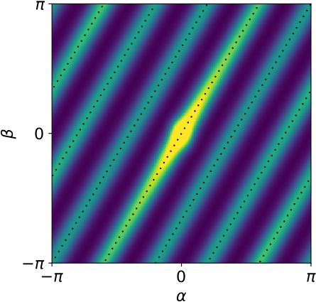
Figure 3: The guiding center paths of fig. 2 represented on tori embedded in a three-sphere
S 3 (whose points satisfy x2 + y 2 + u2 + v 2 = cst). Through stereographic projection, one
can think of this S 3 as R3 plus a point at infinity, so each of the three plots in this figure
depicts one edge mode in what will, eventually,√ be the boundary of a Hall droplet. As in
fig. 2, the anisotropy (7) is ∆ = 1, 5/3 and 2 from left to right.

correlations and the impossibility to rely on known special functions. In order to stream-
line the presentation, detailed asymptotic computations are relegated to appendices B–C.
Correlations of ergodic edge modes are treated separately in section 4.

One-body spectrum. We begin by considering the one-body Hamiltonian H of eq. (3)
with a harmonic trap (5) and magnetic field B = dA = B(dx∧dy+du∧dv). Owing to the
quadratic form of the complete Hamiltonian, including both the Landau term (p − A)2 /2
and the potential V (x), it is in fact possible to diagonalize it exactly: this is shown in
appendix A. However, in keeping with section 2, our approach here will rely on projected
operators in the lowest Landau level (LLL). The ensuing formulas only differ from the
exact results of appendix A by corrections that are tiny in the limit of strong magnetic
fields, so they are eventually harmless for our main points below regarding correlations
(this section and section 4) and entanglement (section 5).
   Choosing symmetric gauge, let A = B(x dy − y dx + u dv − v du)/2. To diagonal-
ize the quantum Hamiltonian
                         √ H, it is then convenient
                                             √       to define dimensionless complex
coordinates z ≡ (x + iy)/ 2`B , w ≡ (u + iv)/ 2`B and annihilation operators
                  z                  z̄                    w                  w̄
             a≡     + ∂z̄ ,    b≡       + ∂z ,        c≡     + ∂w̄ ,     d≡      + ∂w .    (8)
                  2                  2                     2                  2
In these terms, the second class constraint (1) at strong magnetic fields reads a ≈ c ≈ 0
(in addition to their Hermitian conjugates). This is enforced in the quantum theory by
restricting attention to those states for which a|φi = c|φi = 0 [47, chap. 13]. Equivalently,
such states minimize the pure Landau Hamiltonian (p − A)2 /2 = ~B(a† a + c† c + 1) and
span the LLL. The trapping potential (5) is then treated in the framework  of degenerate
perturbation theory, where its LLL projection reads V ≈ ~ω b† b + 1 + ~ω 0 d† d + 1 .


The ensuing approximate one-body energy spectrum is
                                    Em,n = ~ω m + ~ω 0 n                                   (9)
(up to an irrelevant additive constant) and the corresponding normalized eigenfunctions
                                                 1 z m wn −(|z|2 +|w|2 )/2
                          φmn (z, z̄, w, w̄) =    √       e                               (10)
                                                 π m! n!
generalize standard LLL wavefunctions in 2D symmetric gauge. (This also holds without
LLL projection, up to slightly different definitions of (z, w): see the end of appendix A.)

                                                  8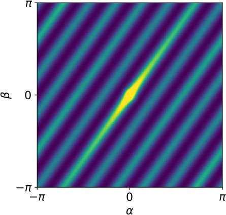
√Note √ that the probability density |φmn | is maximal on the torus where (|z|, |w|) =
                                             2

( m, n). This is consistent with the fact that all guiding center trajectories lie in
such tori (recall section 2). To some extent, it is even possible to build more localized
eigenstates that exhibit individual trajectories, at least provided the ratio (7) is rational:
the energy (9) only depends on the sum ωm + ω 0 n, so Fourier-transforming the wave-
functions (10) along a fixed high-energy shell produces states localized on curves of the
form β = ∆ α + cst. The remainder of this section is devoted to the proof of a similar
localization affecting the correlation function of non-interacting Hall droplets.

Isotropic droplets. Consider a droplet of non-interacting fermions subjected to the
Landau Hamiltonian (3) in an isotropic trap (5), so that the frequency ratio (7) is ∆ = 1.
As in section 2, we assume that the magnetic field is so large that low energy physics is
entirely described by the LLL. The many-body ground state (see fig. 4) then reads
                                          Y
                                  |Ωi =        a†mn |0i                               (11)
                                               m,n∈N
                                               m+n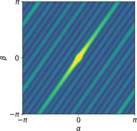
n                 ···························································                m
                                      · ················································································
                                   ········                                                                        ········
                                      ·                                                                                ·

                                                                                                          N
                               Energy

Figure 4: The spectrum (9) of LLL states (10) in an isotropic trap (5). In contrast to the
2D QHE, degeneracies persist despite the trap: wavefunctions φmn with the same value
of m + n have the same energy. The red dots are states that contribute to the many-body
ground state (11). This should be compared with the anisotropic spectrum in fig. 5.

   To begin, recall a general result on the asymptotics of the incomplete gamma function.
Using steepest-descent methods based on the definition of the gamma function as an
integral in the complex plane, a straightforward but lengthy computation shows that the
large N limit of Γ(N, N λeiϕ ), with fixed λ > 0 and ϕ 6= 0, is given by4

                                N →∞                             1 h           iϕ N
                                                                                 i      1 − λe−iϕ
               Γ(N, N λeiϕ ) ∼ Γ(N ) −                               N λeiϕ−λe                        .                         (14)
                                                                 N                  λ2 + 1 − 2λ cos ϕ
The details of this argument are relegated to appendix B. Our goal is now to apply (14) to
the correlation function (13) in the thermodynamic limit N → ∞, with λ = |Z † Z 0 |/N ∼
1. In order to relate the result to the classical trajectories of section 2, we write the
complex coordinates of R4 ∼ = C2 as
                                            iα
                                     z         e cos(θ/2)
                             Z=          ≡r                   ,                       (15)
                                     w         eiβ sin(θ/2)

where r ≥ 0 and θ ∈ [0, π]. The same notation applies to Z 0 (with extra primes), but we
assume without loss of generality that α0 = β 0 = 0 since the correlation (12) only depends
on differences of phases between (z, w) and (z 0 , w0 ). One can then express√the various
ingredients
     √      of eq. (13) in these terms. In order to approach the edge, let r ≡ N + a and
r ≡ N + b, being understood that a, b are finite and fixed in the limit N → ∞. As for
 0

angular coordinates, section 2 suggests that edge modes propagate along (α + β)/2, while
the remaining angles (θ, α − β) parametrize a two-sphere
                                                     √        S 2 . Accordingly, we assume
that α − β and δθ ≡ θ − θ are both of order O(1/ N ), whereupon (14) yields
                        0

                               1   e−i(N −1/2)α    2  2 N        2   2    2
                           0
                  K(Z, Z ) ∼ − 2 √              e−a −b − 8 [(α−β) sin θ+δθ ] .                                                  (16)
                              π i 8πN sin(α/2)
This expression is a key formula for edge correlations in an isotropic droplet. It holds in
the thermodynamic limit N  1 and for α ∼ β 6= 0, excluding in particular the density
regime α = β = 0 (whose asymptotics are radically different).
   Eq. (16) is reminiscent of its 2D cousin (see e.g. [39, eq. (27)]) in two respects: first,
it decays in a Gaussian manner ∝ e−a −b in the radial direction, confirming that edge
                                        2  2

   4
    Eq. (14) actually holds only if λ ≤ 1, or if λ > 1 and |ϕ| > ϕc for some critical value ϕc (see appendix
B). When, instead, λ > 1 and |ϕ| ≤ ϕc , the Γ(N ) on the right-hand side of (14) disappears, but this
does not affect the asymptotics of correlations (13), where Γ(N ) turns out to be negligible anyway.

                                                                         10
n m
····························································································································
·············································································································································
······························································································································
Energy ···············································································································
································································································
·················································································
··································································
···················································
····································
·····················
······
Figure 5: The spectrum (9) for an anisotropic trap with stiffness ratio ∆ = 5/3. As in
fig. 4, red dots highlight the occupied states of the many-body ground state (17).
correlations are localized, to within a magnetic length, on the S 3 boundary. Second, it ex-
hibits a power-law correlation ∝ [sin(α/2)]−1 , characteristic of fermionic 1D CFTs. What
N 2 2 2
distinguishes (16) from its 2D analogue is the additional localization ∝ e− 8 [(α−β) sin θ+δθ ]
on the guiding center trajectory (6) where α = β, which becomes sharper as N increases.
This confirms that 4D edge modes are gapless fermions that effectively propagate along 1D
circles embedded in a 3D sphere. Note that the generalization to d-dimensional isotropic
droplets is straightforward: the correlator is still given by eq. (13) with Z = (z1 · · · zd/2 )t ,
and edge modes are still supported on circles. We shall now extend this result to less
symmetric traps, where the embedding of edge modes in the S 3 boundary is more tangled
than in the Hopf fibration. Along the way we will derive the edge correlation (16) without
relying on the incomplete gamma function.
Rational anisotropic droplets. Let us generalize the asymptotics (16) to arbitrary
anisotropic traps with periodic guiding center trajectories. In the language of section
2, this corresponds to a rational ratio (7), which we write as ∆ = p/q in terms of
coprime integers p, q. We assume, as before, that the magnetic field is so strong that the
many-body ground state only contains one-body states in the LLL, with a spectrum (9).
However, because of the anisotropy, the ground state is no longer given by eq. (11); it
consists instead of wavefunctions (10) whose indices m, n satisfy (see fig. 5)
0 ≤ m + ∆n < N (17)
for some integer N
1 proportional to the Fermi energy. The number of electrons is
thus N 2 /(2∆) in the thermodynamic limit. Owing to (10), the correlation function is
X X (z̄z 0 )m (w̄w0 )n
0
K(x, x ) = φ∗mn (x)φmn (x0 ) ∝ , (18)
m,n∈N m,n∈N
m! n!
m+∆ nβ
10π
Figure 6: Periodic motion on a torus, with ratio-
nal winding p/q, may be seen as the projection of
8π
a trajectory with unit winding on a pq-fold larger
torus. Here we take p/q = 5/3, as in the central
panels of figs. 2–3. As a result, the small torus where 6π
(α, β) ∈ [0, 2π] × [0, 2π] may be seen as a quotient
of the larger torus where (α, β) ∈ [0, 6π] × [0, 10π]
under the action of the group Z3 × Z5 that maps 4π
(α, β) on (α + 2πµ, β + 2πν) with µ = 0, 1, 2 and
ν = 0, 1, ..., 4. The method of images mentioned
in the main text, and exposed in greater detail in 2π
appendix C, exploits this picture to recast edge cor-
relations in an anisotropic trap as a sum of shifted α
correlations in an isotropic trap. 2π 4π 6π
images is depicted in fig. 6; here, we merely state the result. Namely, let the points x, x0
lie on the boundary and write their complex coordinates as
√ √
z = N eiα cos(θ/2), z 0 = N cos(θ/2),
p p (19)
w = N/∆ eiβ sin(θ/2), w0 = N/∆ sin(θ/2).
Note that we choose the same radii and the same azimuth θ for both x and x0 ; this ensures
that both points belong to the same torus in the edge, although radial and azimuthal
corrections can be included similarly to what we did in (16) for isotropic droplets. We
also assume without loss of generality that the complex coordinates of x0 are both real
(this is again because (18) is invariant under independent rotations of z and w), and we
avoid singular cases by restricting attention to θ ∈ (0, π). Under these assumptions, edge
correlations are found to be
q−1 p−1 α+2πµ
X X e−i 2q −N
8 (
α+2πµ− β+2πν
2
) sin2 θ F (θ)
0
K(x, x ) ∼ √ e ∆ (20)
N q sin α+2πµ
µ=0 ν=0 2q
where we omit an overall prefactor (see the exact formula (C.9)) and F (θ) ≡ [sin2 (θ/2) +
cos2 (θ/2)/∆]−1 . The double sum runs over the aforementioned images: periodic motion
with winding p/q on the unit torus lifts into a trajectory with unit winding on a larger
covering torus consisting of pq copies of the initial one (see fig. 6). The coordinates (α, β)
then have periods (2πq, 2πp) on the larger torus; the unit torus follows by identifying
points that differ by an action (α, β) 7→ (α + 2πµ, β + 2πν) of the group Zq × Zp .
Eq. (20) is one of our main results; it is an explicit formula for edge correlations (at
fixed θ) in the case of rational ratios (7). Such correlations are plotted in fig. 7. When
p = q = 1, eq. (20) reproduces the isotropic expression (16) with a = b = δθ = 0. More
generally, (20) implies that edge modes in rational droplets have power-law correlations
localized on classical guiding center trajectories (where β = ∆ α), away from which
12Figure 7: The norm |K(x, x0 )|, computed numerically thanks to eq. (18), for boundary
points whose complex coordinates (19) have θ = π/2. All three plots represent a torus
whose horizontal and vertical axes are respectively α, β. Yellow denotes higher norms,
navy blue lower ones; intermediate colors interpolate. From left to right, anisotropy ratios
are ∆ = 1, 3/2, 5/3 (respectively with 45150, 30200, 27210 particles). The localization
on the guiding center trajectories of fig. 2 (here shown as black dots) is manifest.
they decay in a Gaussian manner. More precisely, if x and x0 do not lie on the same
classical trajectory, the correlator decays exponentially with N . Meanwhile, on a classical
trajectory, the correlator reduces to that of a (1+1)D chiral massless fermion on a circle:
1
K(x, x0 )|β = ∆ α ∼ hΨ† (x)Ψ(x0 )iCFT = L
(21)
sin π L`
π
where ` = `(x, x0 ) is the distance separating x and x0 along √ the
pclassical trajectory; the
latter is diffeomorphic to a circle with total length L = 2πq N cos (θ/2) + ∆ sin (θ/2)
2 2
(in units of the magnetic length). Note that ` is indeed a correct conformal parametriza-
tion of the classical trajectory (6), since the guiding center velocity has constant norm.
4 Ergodic edge modes
Edge correlations in irrational anisotropic traps are challenging: guiding center trajecto-
ries are no longer periodic and the sum over images (20) turns into a series. To resolve
this puzzle, the present section reports a numerical exploration of edge correlations in
irrational traps. A natural proposal will thus emerge for their thermodynamic limiting
form. It involves a function with a fractal-like graph, not unlike the Thomaé function,
that may be seen as an irrational limit of the strict N = ∞ version of the rational formula
(20). In practice, the correlation function of ergodic edge modes then decays as a power
law along classical trajectories, while it falls off sharply along transverse directions.
Continued fractions and numerics. In order to build intuition on irrational droplets,
it will be helpful to approximate irrational ratios (7) by sequences of rational numbers;
this can be done with continued fractions. An example √ that we will use throughout this
section is the continued fraction representation of ∆ = 2:
√ 1
2=1+ 1 ≡ [1, 2, 2, 2, 2, . . .]. (22)
2+ 1
2+ 2+···
13Figure 8: Numerical computations of the norm |K(x, x0 )| given by (18), for points (19) on
an edge torus at θ = π/2. The color coding is the same as in fig. 7. From
√ left to right, the
ratio (7) provides successive continued fraction approximations of 2, namely ∆ = 7/5,
∆ = 17/12, and ∆ = 41/29 (respectively with 129043, 127553 and 127822 particles).
Classical trajectories become more and more difficult to distinguish as ∆ converges to an
irrational value, motivating the more accurate ‘slice’ plots in fig. 9 below.
√
Successive approximations of 2 are obtained by truncating this sequence, giving 3/2,
7/5, 17/12, 41/29, etc. A similar rewriting applies to any irrational number; it is optimal
in the sense that (i) truncated approximations given by continued fractions converge
exponentially fast with the order of truncation, (ii) if a rational approximation p0 /q 0 is
closer to ∆ ∈
/ Q than some truncated continued fraction p/q, then q 0 > q [50].
This approximation algorithm applies to edge correlations in anisotropic droplets: it
is illustrated
√ in figure 8 for three truncations of the continued fraction representation
√ of
∆ = 2. Notice that correlations involving successive approximations of 2 become
more and more ergodic, with the true limit (if it exists at all) difficult to guess. In fact,
much sharper statements about edge correlations are obtained by analysing density plots
through one-dimensional ‘slices’ — e.g. by setting β to some constant value — which one
can roughly think of as quantum analogues of Poincaré sections. This is done in fig. 9 at
β = 0. In contrast to fig. 8, it is then apparent that correlations in the thermodynamic
limit are far from uniform, even in irrational droplets. The problem thus becomes to find
the limiting form of these correlations.
Fractal correlations. The correlations of ergodic edge modes with anisotropy ∆ ∈ / Q
can be inferred as follows. Starting from the rational formula (20), normalize it in such a
way that its strict thermodynamic limit (N = ∞) be finite and non-trivial. Then consider
a sequence of rational anisotropies that converges to ∆; the limit of their correlation
functions at N = ∞ is the sought-for ergodic correlation function. The remainder of this
section explains this procedure in greater detail.
Recall that eq. (20)√exhibits a Gaussian localization of edge modes on classical trajec-
tories, with width 1/ N . Accordingly, define a rescaled (norm of the) correlator
√
K(α, β) ≡ lim N K(x, x0 ) , (23)
N →∞
where it is understood that x, x0 are two points on the same edge torus, with complex
coordinates (19). This scaling may be seen as a 4D analogue of the well known (chord
length) conformal scaling of edge correlations in circular 2D droplets. Our goal is thus to
14N=350 N=350
0.08 N=700 0.08 N=700
N=1400 N=1400
N K(z, w|zei , w)|
N K(z, w|zei , w)|
N=2800 N=2800
0.06 0.06
0.04 0.04
0.02 0.02
2|
2|
0.00 0 0.00 0
N=350 N=350
0.08 N=700 0.08 N=700
N=1400 N=1400
N K(z, w|zei , w)|
N K(z, w|zei , w)|
N=2800 N=2800
0.06 0.06
0.04 0.04
0.02 0.02
2|
2|
0.00 0 0.00 0
√
Figure 9: The rescaled correlator N |K(x, x0 )| given by (18), for points (19) on the
slice β = 0 of an edge torus at θ = π/2. Black dots denote the maxima of correlations
predicted by the limiting function (24).
√ The four panels have anisotropy ratios providing
different rational approximations of 2: from√ left to right, ∆ = 7/5 and ∆ = 17/12 in
the top panels, while ∆ = 41/29 and ∆ = 2 in the bottom panels. Each plot displays
several values of N ; the largest corresponds to over 2 million particles. The correlator
does not seem to converge to a smooth function in the thermodynamic limit N → ∞; it
becomes instead more ragged at shorter distance scales.
evaluate the limiting correlation (23), seen as a function of α and labelled parametrically
by (∆, θ, β). The hope is that this limit works in both rational and irrational droplets,
eventually reproducing the ‘slice’ plots of fig. 9.
In rational droplets, the limit (23) is readily found thanks to eq. (20) for edge correla-
tions. Indeed, at large N , the various Gaussians appearing in the sum over images (20)
have separate supports, so the limit N → ∞ turns each such Gaussian into a pointwise
indicator function. The rescaled correlator (23) thus takes non-zero values only when
α = (β + 2πν)/∆ mod 2π for some integer ν, that is, exactly on the classical trajectory.
The actual value is determined by the power-law decay of (20), yielding
1 if α = β+2πν mod 2π for some ν ∈ {0, . . . , p − 1},
β+2πν ∆
K(α, β) ∝ q| sin( 2p
)| (24)
0 otherwise
up to a θ-dependent normalization (the exact result, shown in eq. (C.11), follows from
the detailed rational formula (C.9)). This expression can trivially be extended to a 2π-
15periodic function on R. On [0, 2π), it vanishes for almost all α, except at max(p, q) points
where it is finite. A mild exception occurs for β = 0 mod 2π, since the points x, x0 then
coincide at α = 0 mod 2π, where K(α, β) = ∞.
The function (24) at β = 0 is displayed with black bullets in fig. 9, for various ∆’s and
α ∈ [−π, π]. As can be seen, the agreement with numerical data for large but finite N
is perfect. The agreement even seems to extend to irrational droplets, so it is tempting
to still rely on (24) in that case. This can be done in two ways: either take a sequence
of rational ratios ∆k converging to ∆ when k → ∞ (e.g. using continued fractions) and
conjecture that K∆ = limk→∞ K∆k ; or take the actual irrational limit of (24) to obtain
1 if α = β+2πν
mod 2π for some ν ∈ Z,
|β + 2πν| ∆
K(α, β) ∝ (25)
0 otherwise.
(Normalization is omitted as in (24); the exact result is given in eq. (C.12).) The function
(25) is thus well-defined but highly irregular: it vanishes almost everywhere, except on
the countable intersection between the β slice and a guiding center trajectory, where it is
discontinuous. This is √reminiscent of the Thomaé function and other fractal-like graphs.
A plot of K for ∆ = 2 is shown in fig. 9 (bottom right) and fig. 10, confirming the
perfect agreement between numerical correlations at finite N and the prediction (25).
0.09
∆ = 7/5
0.08
∆ = 17/12
0.07 ∆ = 41/29
√
0.06 ∆= 2
π 2 K(α, β = 0)
0.05
0.04
0.03
0.02
0.01
0
−π 0 π
α
Figure 10: Conjecture
√ (25) for the rescaled correlator K (defined in (23)) in the irrational
case, here for ∆ = 2 and θ = π/2, and comparison with continued fraction approxima-
tions. Notice the fractal-like structure of the graph: sequences of three successive peaks
repeat themselves at different scales throughout the plot.
Similar to before, the correlator (25) boils down to the one-dimensional CFT result for
free fermions on the infinite line, as long as x and x0 lie on the same classical trajectory:
1
K(x, x0 ) ∼ hΨ† (x)Ψ(x0 )iCFT = (26)
`
where ` is the distance separating x and x0 along the trajectory. This is nothing but
the L → ∞ limit of eq. (21). The interpretation is straightforward: an edge excitation
born at (0, 0) propagates along its torus at constant velocity, and the correlation (25) is
16proportional to the inverse of the time it takes for it to reach the point (α, β); this time
is infinite if (α, β) does not belong to the guiding center trajectory passing through the
origin. This is illustrated in fig. 11, which shows side by side a numerical√evaluation of
the edge correlator along the classical trajectory, for ∆ = 17/12 and ∆ = 2. As can be
seen, the agreement is excellent.
N=200 N=200
0.08 N=400 0.08 N=400
N=800 N=800
N K(z, w|z( ), w( )|
N K(z, w|z( ), w( )|
N=1600 N=1600
0.06 CFT 0.06 CFT
0.04 0.04
0.02 0.02
2|
0.00 0 2| 0.00 0 1 2 3 4 5 6 7 8 9 10
L/2 L
/2 N
Figure 11: Numerical computation of the rescaled correlator along the classical trajec-
tory, for several values of N . Left: rational case ∆ = 17/12,√perfectly reproducing the
CFT correlator (21) on a circle. Right: irrational case ∆ = 2, with integer abscissae
indicating the number of times the trajectory wraps around the torus. The agreement
with the CFT correlator (26) on an infinite line is excellent. Notice the bumps in the
curves with relatively small N : these are finite-size effects, due to the fact that the Gaus-
sian spread is too large for small N and that the classical trajectory is not yet sharply
resolved; such pathologies disappear at large N .
We conclude this section with two technical remarks. First, we stress that the ragged,
fractal-like function (25) only emerges in the strict thermodynamic limit. This implies in
practice that any finite droplet, no matter how large, has edge correlations that will at
best be approximately given by (25); for any finite N , one may in fact assume that the
anisotropy ratio (7) is rational (albeit with a numerator and denominator that grow with
N ). Second, notice that we refer to (25) as a conjecture rather than a proven statement.
This is because our derivation of (25) relied on the rational correlations (20), followed
by a strict large N limit, followed in turn by an irrational limit. By contrast, a proper
proof of (25) would assume an irrational ratio (7) at the outset, then find asymptotics
of correlations in the thermodynamic limit. We will not attempt to perform such a
computation here, and now return instead to the comforting realm of rational droplets.
5 Quantum entanglement
In sections 2–4 we analysed the edge modes of a 4D Hall droplet using their boundary cor-
relator, exhibiting edge conduction channels localized on classical guiding center trajecto-
ries. It is rather natural to presume that these channels are decoupled, and therefore can
be described by a collection of independent (1+1)D CFTs. We now confirm this intuition
thanks to the ground state entanglement of various spatial subregions. Indeed, entangle-
ment entropy is a well-established probe of quantum matter and of gapless edge modes
17in particular, as was shown e.g. in 2D droplets [39, 51], at interfaces between fractional
quantum Hall states [52–54], or in 3D topological insulators with hinge modes [55, 56].
Since we are dealing here with non-interacting fermions, calculations simplify consider-
ably [40–44]: one can relate the entanglement spectrum to that of a subregion-restricted
correlation matrix, reducing the computation of many-body entanglement to a one-body
problem.
We mostly focus on isotropic droplets (∆ = 1) from now on, being understood that our
conclusions extend to rational anisotropic droplets. Edge modes then propagate along
Hopf fibers in S 3 , as in fig. 1. Two kinds of simple entangling regions will be considered,
where analytical calculations can be carried out to the end. The first are devised so as
to avoid crossing any boundary fiber; their entanglement entropy will turn out to receive
no contribution from edge modes, confirming that the latter are indeed decoupled. By
contrast, the entanglement entropy of regions that deliberately cut through fibers will
include logarithmic terms, characteristic of gapless 1D systems [57–59], multiplied by a
CFT central charge. These considerations are 4D analogues of what has been done in [39]
for 2D droplets, and extend the recent results of [27, 60] by including boundary effects.
Spherical cap and area law. Here we consider a subregion of R4 whose boundary
crosses none of the S 1 fibers supporting edge modes. For simplicity, we choose a highly
symmetric region, such that we will in fact be able to evaluate explicitly the whole entan-
glement spectrum. An asymptotic calculation (detailed in appendix D) then produces the
thermodynamic limit of entanglement entropy, exhibiting the area law of gapped systems.
The first subleading correction of this result, normally containing the contribution of edge
modes, turns out to vanish. In this sense, periodic edge modes truly are independent:
each propagates on its own fiber, free of correlations with its neighbors.
Consider an isotropic droplet and label points in R4 ∼
= C2 by coordinates (15). In these
terms, a ‘spherical cap’ in R is a region where (see fig. 12)
4
r ∈ [R, +∞), θ ∈ [0, γ], α ∈ [0, 2π], β ∈ [0, 2π], (27)
with R an ‘inner radius’ and γ ∈ (0, π) an azimuth. The coordinates (θ, α − β) thus cover
a spherical cap with opening γ on S 2 (hence the terminology); S 1 fibers with coordinate
(α + β)/2 are covered entirely. Equivalently, the region (27) is the product of a semi-
infinite radial interval with a solid torus whose surface is spanned by (α, β).
Sections 2–3 ensure that edge mode do not propagate across the boundary of the cap
(27). Entanglement entropy should therefore satisfy both a bulk area law and an edge area
law. Accordingly, let us evaluate, for future reference, the volume of the cap’s boundary
and the area of its intersection with the edge of the droplet. The boundary consists of
two pieces (r = R and θ = γ) with volume forms
r3 r2
ωr=cst = sin θ dθ dα dβ, ωθ=cst = sin θ dr dα dβ, (28)
4 2
so its total volume, given some outer radius R0 , is
R03 − R3
Area(cap) = 2π (R + R ) sin (γ/2) +
2 03 3 2
sin γ . (29)
3
The first term is due to the angular integral of ωr=R and ωr=R0 , while the second stems
from the radial integral of ωθ=γ . (In particular, when γ = π, eq. (29) reduces to the
18You can also read