Upside-down fluxes Down Under: CO2 net sink in winter and net source in summer in a temperate evergreen broadleaf forest - Biogeosciences
←
→
Page content transcription
If your browser does not render page correctly, please read the page content below
Biogeosciences, 15, 3703–3716, 2018
https://doi.org/10.5194/bg-15-3703-2018
© Author(s) 2018. This work is distributed under
the Creative Commons Attribution 4.0 License.

Upside-down fluxes Down Under: CO2 net sink in winter and net
source in summer in a temperate evergreen broadleaf forest
Alexandre A. Renchon1 , Anne Griebel1 , Daniel Metzen1 , Christopher A. Williams2 , Belinda Medlyn1 ,
Remko A. Duursma1 , Craig V. M. Barton1 , Chelsea Maier1 , Matthias M. Boer1 , Peter Isaac3 , David Tissue1 ,
Victor Resco de Dios4 , and Elise Pendall1
1 Hawkesbury  Institute for the Environment, Western Sydney University, Penrith, NSW, Australia
2 GraduateSchool of Geography, Clark University, Worcester, Massachusetts 01610, USA
3 CSIRO Oceans & Atmosphere Flagship, Yarralumla, ACT, 2600, Australia
4 Department of Crop and Forest Sciences-AGROTECNIO Center, University of Lleida, 25198 Lleida, Spain

Correspondence: Alexandre A. Renchon (a.renchon@gmail.com)

Received: 7 December 2017 – Discussion started: 2 January 2018
Revised: 18 April 2018 – Accepted: 10 May 2018 – Published: 19 June 2018

Abstract. Predicting the seasonal dynamics of ecosystem          had larger seasonal amplitude compared to GPP, and there-
carbon fluxes is challenging in broadleaved evergreen forests    fore drove the seasonal variation of NEE. Because summer
because of their moderate climates and subtle changes in         carbon uptake may become increasingly limited by atmo-
canopy phenology. We assessed the climatic and biotic            spheric demand and high temperature, and because ecosys-
drivers of the seasonality of net ecosystem–atmosphere CO2       tem respiration could be enhanced by rising temperatures,
exchange (NEE) of a eucalyptus-dominated forest near Syd-        our results suggest the potential for large-scale seasonal
ney, Australia, using the eddy covariance method. The cli-       shifts in NEE in sclerophyll vegetation under climate change.
mate is characterised by a mean annual precipitation of
800 mm and a mean annual temperature of 18 ◦ C, hot sum-
mers and mild winters, with highly variable precipitation.
In the 4-year study, the ecosystem was a sink each year          1   Introduction
(−225 g C m−2 yr−1 on average, with a standard deviation of
108 g C m−2 yr−1 ); inter-annual variations were not related     Forests and semi-arid biomes are responsible for the major-
to meteorological conditions. Daily net C uptake was always      ity of global carbon storage by terrestrial ecosystems (Dixon
detected during the cooler, drier winter months (June through    et al., 1994; Pan et al., 2011; Poulter et al., 2014; Schimel et
August), while net C loss occurred during the warmer, wet-       al., 2001). Photosynthesis and respiration by these biomes
ter summer months (December through February). Gross pri-        strongly influence the seasonal cycle of atmospheric CO2
mary productivity (GPP) seasonality was low, despite longer      (Baldocchi et al., 2016; Keeling et al., 2005). Continuous
days with higher light intensity in summer, because vapour       measurements of land–atmosphere exchanges of carbon, en-
pressure deficit (D) and air temperature (Ta ) restricted sur-   ergy and water provide insights into the seasonality of for-
face conductance during summer while winter temperatures         est ecosystem processes, which are driven by the interac-
were still high enough to support photosynthesis. Maximum        tions of climate, plant physiology and forest composition and
GPP during ideal environmental conditions was significantly      structure (Xia et al., 2015). Net ecosystem exchange (NEE)
correlated with remotely sensed enhanced vegetation index        seasonality is relatively well understood in cool-temperate
(EVI; r 2 = 0.46) and with canopy leaf area index (LAI;          ecosystems; deciduous trees can only photosynthesise when
r 2 = 0.29), which increased rapidly after mid-summer rain-      they have leaves and NEE dynamics are thus principally in-
fall events. Ecosystem respiration (ER) was highest during       fluenced by the phenology of canopy processes. NEE of de-
summer in wet soils and lowest during winter months. ER          ciduous forests thus has a more pronounced seasonality than
                                                                 that of evergreen conifer forests at similar latitudes (Novick

Published by Copernicus Publications on behalf of the European Geosciences Union.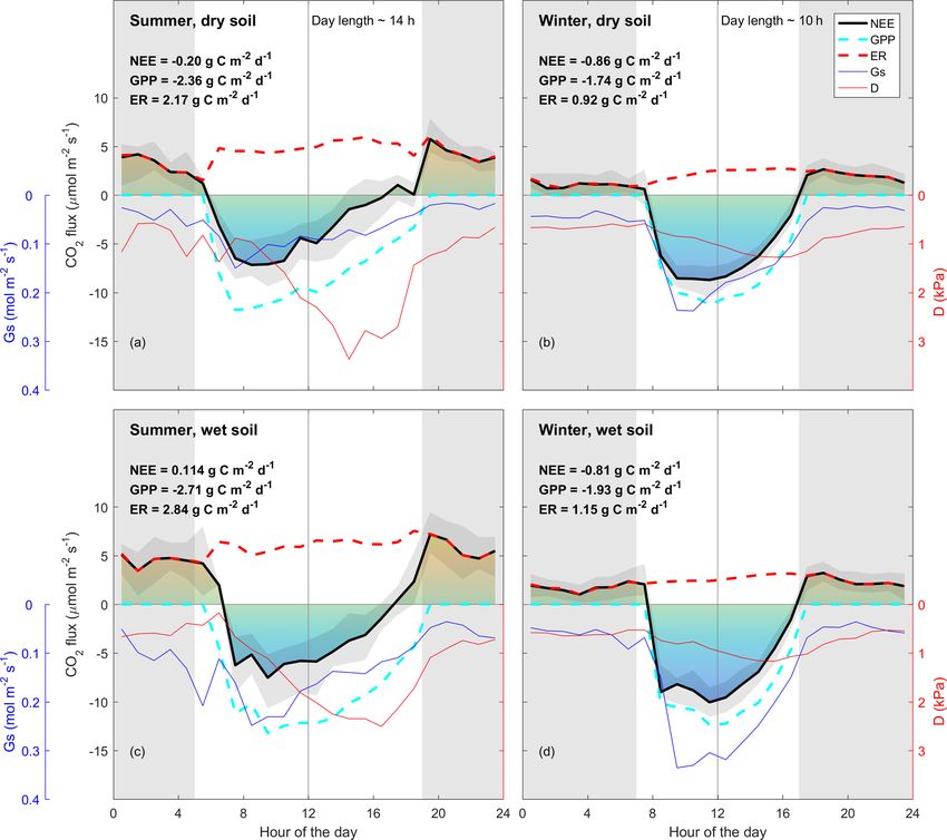
3704                                                                   A. A. Renchon et al.: Upside-down fluxes Down Under

et al., 2015). For high-latitude evergreen conifer forests, NEE    malised difference vegetation index (NDVI) has successfully
seasonality is strongly limited by cold temperature limita-        explained variability in photosynthetic capacity in Mediter-
tion of photosynthesis (Kolari et al., 2007) and respiration. In   ranean, mulga and savanna ecosystems (Restrepo-Coupe et
contrast, seasonality of NEE in evergreen broadleaf forests,       al., 2016).
typically occurring in warm-temperate and tropical regions,           The environmental and biotic controls on the seasonal dy-
is much less well understood (Restrepo-Coupe et al., 2017;         namics of ecosystem fluxes in broadleaved evergreen forests
Wu et al., 2016).                                                  are still poorly understood. Our objective was to determine
   The seasonality of gross primary productivity (GPP) in          the seasonality of ecosystem CO2 and H2 O fluxes in a
evergreen broadleaf forests may be driven by climate (e.g.         dry sclerophyll Eucalyptus forest; we evaluated the role of
dry/wet seasons) and/or by canopy dynamics (Wu et al.,             environmental drivers (photosynthetic photon flux density,
2016). In tropical evergreen forests, air temperature and day      PPFD; Ta ; soil water content, SWC; D) and canopy dynam-
length are similar seasonally, but precipitation seasonality       ics (as measured with EVI, LAI, litter fall and leaf age) in
can be strong, with higher radiation and temperature (1 or         regulating the seasonal patterns of NEE, GPP, ecosystem res-
2 ◦ C higher) in the dry season (Trenberth, 1983; Windsor,         piration (ER), evapotranspiration (ET) and surface conduc-
1990). Counter-intuitively, GPP can be higher during the dry       tance (Gs ) in an evergreen forest near Sydney, Australia. We
season, as cloud cover may limit productivity in the wet sea-      also compared leaf-level to ecosystem-level water and carbon
son (Graham et al., 2003; Hutyra et al., 2007; Saleska et          exchange in response to drivers, in order to gain confidence
al., 2003). Canopy dynamics can be an important determi-           in our results and gain insights into the emergent properties
nant of GPP seasonality in evergreen broadleaf forests; al-        from leaf to ecosystem scale. We hypothesised that canopy
though leaves are present in the canopy year-round in ever-        phenology (LAI and leaf age) explains temporal variation in
green canopies, leaf area index (LAI) may show considerable        photosynthetic capacity (PC) and Gs . We anticipated that the
temporal variability seasonally as new leaves are produced         ecosystem would be a carbon sink all year long.
and old leaves die, especially during leaf flush and senes-
cence periods (Duursma et al., 2016; Wu et al., 2016). Both
leaf light use efficiency and water use efficiency may vary
as leaves age: young leaves and old leaves are less efficient      2     Materials and methods
than mature leaves, reflecting changes in photosynthetic ca-
pacity (Wilson et al., 2001; Wu et al., 2016). The timing of       2.1    Site description
leaf flush and senescence can depend on the environment and
on species; environmental stress, such as drought, can induce      The field site is the Cumberland Plain (AU-Cum in Fluxnet)
the process of senescence (Lim et al., 2007; Munné-Bosch           forest SuperSite (Resco de Dios et al., 2015) of the Australian
and Alegre, 2004).                                                 Terrestrial Ecosystem Research Network (http://www.ozflux.
   In temperate evergreen broadleaved forests, such as             org.au, last access: 12 June 2018), located 50 km west of Syd-
eucalypt-dominated sclerophyll vegetation in Australia, pre-       ney, Australia, at 23 m elevation, on a nearly flat floodplain of
cipitation can be seasonal or aseasonal; furthermore, day          the Nepean–Hawkesbury River (latitude −33.61518; longi-
length and temperature vary significantly between winter and       tude 150.72362). Mean mid-afternoon (15:00 local standard
summer. GPP can be limited by frost during winter and by           time) temperature is 18 ◦ C (max. 28.5 ◦ C in January and min.
drought during summer. Atmospheric demand indicated by             16.5 ◦ C in July) and average precipitation is 801 mm yr−1
high vapour pressure deficit (D) and soil drought have dif-        (mean monthly max. is 96 mm in January, and min. is 42 mm
ferent impacts on GPP, but they can interact to impact sur-        in September). The soil is classified as a Kandosol and con-
face conductance (Gs ; Medlyn et al., 2011; Novick et al.,         sists of a fine sandy loam A horizon (0–8 cm) over clay
2016). In Australia’s temperate eucalypt forests, canopy re-       to clay loam subsoil (8–40 cm), with pH of 5 to 6 and up
juvenation takes place in summer and is linked to heavy rain-      to 5 % organic C in the top 10 cm (Karan et al., 2016).
fall events (Duursma et al., 2016). However, since leaf flush-     The flux tower is in a mature dry sclerophyll forest, with
ing and shedding occur simultaneously in eucalypt canopies         140 Mg C ha−1 aboveground biomass and a stand density
(Duursma et al., 2016; Pook, 1984), the overall canopy vol-        of ∼ 500 trees ha−1 . The stand hosts a large population of
ume can remain stable while the distribution of canopy             mistletoe (Amyema miquelii), which decreases in abundance
volume changes with height (Griebel et al., 2015). Euca-           with increasing distance from the flux tower. The canopy
lypt forests in southeast Australia have been found to act         structure comprises three strata, and the predominant canopy
as carbon sinks all year long, with greater uptake in sum-         tree species are Eucalyptus moluccana and E. fibrosa. While
mer (Hinko-Najera et al., 2017; van Gorsel et al., 2013).          individual trees can exceed 25 m height, an airborne lidar sur-
Although canopy characteristics are key to understanding           vey from November 2015 indicates an average canopy height
ecosystem fluxes, their dynamics in Australian ecosystems          of ∼ 24 m within a 300 m radius of the flux tower (Fig. S1 in
can be particularly challenging to detect using standard veg-      the Supplement). The mid-canopy stratum (5–12 m) is dom-
etation indices (Moore et al., 2016). Nevertheless, the nor-       inated by Melaleuca decora and the understory is dominated

Biogeosciences, 15, 3703–3716, 2018                                                     www.biogeosciences.net/15/3703/2018/
A. A. Renchon et al.: Upside-down fluxes Down Under                                                                     3705

by Bursaria spinosa with various shrubs, forbs, grasses and      hence no clear threshold (Fig. S2), so we used a threshold of
ferns present in lower abundance.                                0.2 m s−1 to be conservative.
                                                                    The calculation of each term, and the assumptions required
2.2   Environmental measurements                                 for them to be representative of each half-hour flux are de-
                                                                 tailed below.
Air temperature (Ta ) and relative humidity (RH) were mea-
sured using HMP45C and HMP155A (Vaisala, Vantaa, Fin-            2.4   Vertical turbulent flux (FCT )
land) sensors at 7 and 29 m heights respectively. Vapour
pressure deficit (D) was estimated from Ta and RH. The           The vertical turbulent fluxes of CO2 (FCT , µmol m−2 s−1 )
PPFD above the canopy (µmol m−2 s−1 ) was measured us-           and water (FWT , mmol m−2 s−1 ) were measured using the
ing an LI190SB (Licor Inc., Lincoln, NE, USA), and incom-        eddy covariance method (Baldocchi et al., 1988). Density
ing and outgoing shortwave and longwave radiation were           (c) of CO2 or water vapour (open-path IRGA, LI-7500A,
measured using a CNR4 radiometer (Kipp & Zonen, Delft,           Licor Inc., Lincoln, NE, USA) and vertical wind speed
the Netherlands). Ancillary data were logged on CR1000 or        (w; CSAT 3D sonic anemometer, Campbell Scientific, Lo-
CR3000 data loggers (Campbell Scientific, Logan, UT, USA)        gan, UT, USA) were measured at 10 Hz frequency at 29 m
at 30 min intervals. Mixing ratios of CO2 in air were also       above the ground, and logged on a CR-3000 data logger
measured at 0.5, 1, 2, 3.5, 7, 12, 20 and 29 m above the         (Campbell Scientific, Logan, UT, USA). Vertical turbulent
soil surface using a LI840A Gas Analyzer (Licor Inc., Lin-       fluxes were calculated from the 10 Hz data, using EddyPro©
coln, NE, USA); data from each height were logged on a           software. Statistical tests for raw data screening included
CR1000 data logger once every 30 min (1 min air sampling         spike count/removal, amplitude resolution, drop-outs, ab-
per height).                                                     solute limits and skewness and kurtosis tests (Vickers and
   Ground heat flux and soil moisture were averaged between      Mahrt, 1997). Low- and high-frequency spectral correction
two locations to represent the variable shading in the tower     followed Moncrieff et al. (2004, 1997). The calculation al-
footprint. One location had a HFP01 heat flux plate and the      lowed for up to 10 % of missing 10 Hz data. Fluxes were ro-
other had a self-calibrating heat flux plate (HFP01SC; Huk-      tated into the natural wind coordinate system using the dou-
seflux, XJ Delft, the Netherlands) installed at 8 cm below the   ble rotation method (Wilczak et al., 2001). We compensated
soil surface. The heat flux plates were paired with a CS616      for time lags between the sonic and IRGA by using covari-
water content reflectometer (Campbell Scientific, Logan UT)      ance maximisation, within a window of plausible time lags
installed horizontally at 5 cm below the soil surface and an     (Fan et al., 1990). We applied the block averaging method
averaging thermocouple (model TCAV, Campbell Scientific,         to calculate each half-hour average and fluctuation relative
Logan, UT, USA) installed with thermocouples at 2 and 6 cm       to the average, to calculate the covariance (Gash and Culf,
below the soil surface for each pair. Another CS616 was in-      1996). Density fluctuations in the air volume were corrected
stalled vertically to measure average soil water content from    using the WPL terms (Webb et al., 1980). Each half-hourly
7 to 37 cm (CS616). Rainfall was measured at an open area        flux was associated with a QC flag (0: good quality; 1: keep
with a tipping bucket 2 km away from the study site.             for integrations, discard for empirical relationships; 2: re-
                                                                 move from the data); these flags accounted for stationarity
2.3   Net ecosystem exchange                                     tests and turbulence development tests which are required for
                                                                 good turbulent flux measurements (Foken et al., 2004). In our
Continuous land–atmosphere exchange of CO2 mass (NEE)            4-year record, 51 % of FCT fluxes had a flag of 0, 32 % had a
was quantified from direct measurements of the different         flag of 1 and 17 % had a flag of 2. Although the tower height
components of the theoretical mass balance of CO2 in a con-      (29 m) is rather close to the average canopy height (24 m),
trol volume:                                                     cospectra analysis showed good quality turbulent fluxes (the
                                                                 high frequency followed the −4/3 slope; thus we did not find
NEE = FCT + FCS ,                                          (1)   any indications of systematic dampening in the cospectra; see
                                                                 Fig. S3).
where FCT is the vertical turbulent exchange flux, and FCS
                                                                 2.5   Storage flux (FCS )
is the change in storage flux. Advection fluxes are assumed
negligible when atmospheric turbulence is sufficient (Aubi-      The change in storage flux (FCS , µmol m−2 s−1 ) was mea-
net et al., 2012; Baldocchi et al., 1988), and when quality      sured using a CO2 profiler system, such that change of stor-
control (QC) flags of stationarity and turbulence develop-       age flux timestamp was the same as the turbulent flux times-
ment test were good (Foken et al., 2004). We used change-        tamp.
point detection of the friction velocity (u∗ ) threshold (Barr
et al., 2013) to determine the turbulence threshold above
which NEE (the sum of FCT and FCS ) is independent of u∗ .
However, we found no clear dependence of NEE on u∗ and

www.biogeosciences.net/15/3703/2018/                                                   Biogeosciences, 15, 3703–3716, 2018
3706 A. A. Renchon et al.: Upside-down fluxes Down Under
The change in storage flux was calculated as (Aubinet et with the highest feature importance for each flux and com-
al., 2001): pared the gap-filling performance of the neural network for
each flux with the performance based on an educated guess
Zh of potential relevant drivers. We selected the variable array
Pa dC(z)
FCS = dz, (2) with the highest Pearson correlation coefficient (r) and low-
R Ta dt
0 est root mean square error (RMSE) for gap-filling in PyFlux-
Pro, which identified net radiation (Rn ), SWC, soil tempera-
where Pa is the atmospheric pressure (Pa ), Ta is the tem- ture (Ts ), wind speed (ws ) and vapour pressure deficit (D) for
perature (K), R is the molar gas constant and C(z) is CO2 λE (r = 0.93, RMSE = 32.0); down-welling shortwave radi-
(µmol m−3 ) at the height z. CO2 is measured in ppm and con- ation (Fsd ), air temperature (Ta ), Ts , ws , SWC and D for H
verted to µmol m−3 using ideal gas law equation, where the (r = 0.97, RMSE = 23.1); Fsd , D, Ta , Ts and SWC for NEE
air temperature and air pressure at each inlet are estimated (r = 0.87, RMSE = 4.04). To gap-fill ER, all nocturnal ob-
from a linear interpolation between sensors at the top of the servational data (at night, we assume GPP = 0 so NEE = ER)
tower (29 m) and sensors at the bottom of the tower (7 m). As that passed all QC checks and the u∗ filter were modelled us-
we only measure a limited number of heights, in practice this ing Ts , Ta and SWC as drivers in SOLO on the full dataset
equation becomes with 10 nodes and 500 iterations. Lastly, this gap-filled ER
was used to infer GPP as the result of NEE − ER.
1C
FCS = × zk=1
1t k=1 2.7 Flux footprint
Xn 1C 1C zk − zk−1
+ + × , (3) We analysed the footprint climatology of Cumberland Plain
k=2 1t k 1t k−1 2 site according to Kormann and Meixner (2001), using the
R-Package “FREddyPro” (Fig. S5). We assumed that the
where C is CO2 (µmol m−3 ) and t is time (s; 1C/1t is the ecosystem within the footprint was homogeneous for the pur-
variation of C over 30 min), z is the height (m) and k [1 to pose of this study and found that, after u∗ filtering, CO2 tur-
n = 8] represents each inlet. We flagged and replaced the bulent fluxes (FCT ) originated from the footprint of interest.
storage flux with a one-point approximation during profiler
outages (25 % of the 4-year record), using the change in CO2 2.8 Energy balance
at 29 m height over 30 min as derived in EddyPro (Aubinet
et al., 2001). These data were not used for empirical relation- We evaluated the energy balance closure with the ratio of
ships, but kept for annual sum calculations. Storage flux of available energy (Rn − soil heat flux, G) to the sum of tur-
water vapour was assumed to be negligible. For visualisation bulent heat fluxes (λE + H ). On a daily basis, the energy
of the diurnal course of storage flux and turbulent flux, see balance closure was 70 % (Fig. S6), consistent with the well-
Fig. S4. known and common issue of a lack of closure (Foken, 2008;
Foken et al., 2006; Wilson et al., 2002). We did not use the
2.6 Gap-filling of environmental variables and NEE criteria that closure had to be met for the reported fluxes.
separation into gross fluxes
2.9 Surface conductance
We used the PyFluxPro software for gap-filling climatic vari-
ables and fluxes, and for partitioning the NEE into GPP and Surface conductance (Gs ) was derived by inverting the
ER (Isaac et al., 2017). We only used observational data that Penman–Monteith equation (Monteith, 1965):
passed the steady state and developed turbulence tests for γ λEga
gap-filling and for partitioning (QC flags of 0 and 1; Foken et Gs = , (4)
1Rn + ρCp Dga − λE (1 + γ )
al., 2004). In brief, gaps in climate variables were filled fol-
lowing the hierarchy of using variables provided from (1) au- where γ is the temperature-dependent psychrometric con-
tomatic weather stations from the closest weather station, stant (kPa K−1 ), λE is the latent heat flux (W m−2 ), 1 is the
(2) numerical weather prediction model outputs (ACCESS temperature-dependent slope of the saturation–vapour pres-
regional, 12.5 km grid size provided by the Bureau of Mete- sure curve (kPa K−1 ), Rn is net radiation (W m−2 ), ρ is the
orology) and lastly (3) monthly mean values from the site- dry air density (kg m−3 ), D is vapour pressure deficit (kPa),
specific climatology. In the next step the continuous climate Cp is the specific heat of air (J kg−1 K−1 ) and ga is the bulk
variables were used to fill all fluxes by utilising the embed- aerodynamic conductance, formulated as an empirical rela-
ded SOLO neural network with 25 nodes and 500 iterations tion of mean horizontal wind speed (U , m s−1 ) and friction
on monthly windows. We used the random forest method velocity (u∗ , m s−1 ; Thom, 1972):
(Breiman, 2001) to determine and rank potential explana-
tory variables for explaining latent heat flux (λE), sensible 1
ga = U −0.67
. (5)
heat flux (H ) and NEE. We then selected the five variables 2 + 6.2u∗
u∗
Biogeosciences, 15, 3703–3716, 2018 www.biogeosciences.net/15/3703/2018/A. A. Renchon et al.: Upside-down fluxes Down Under 3707
In the analysis for Gs , we were interested in transpiration (T ) 2.12 Leaf gas exchange spot measurements
rather than evaporation (E), so we excluded data if precipi-
tation exceeded 1 mm in the past 2 days, 0.5 mm in the past We used previously published data of spot leaf gas exchange
24 h and 0.2 mm in the past 12 h (Knauer et al., 2015). We measurements in a nearby site for comparison with ecosys-
assumed that evaporation (E) was negligible using these cri- tem fluxes (Gimeno et al., 2016).
teria (Knauer et al., 2018), which excluded 40 % of the data.
2.13 Remotely sensed land surface greenness
2.10 Dynamics of canopy phenology (leaf area index,
and litter and leaf production) and photosynthetic Normalised difference vegetation index (NDVI) and En-
capacity hanced Vegetation Index (EVI) values were derived from the
MODIS Terra Vegetation Indices 16-Day L3 Global 250 m
We evaluated the dynamics of canopy LAI by measur- product (MOD13Q1), which uses atmospherically corrected
ing canopy light transmittance with three under-canopy surface reflectance masked for water, clouds, heavy aerosols,
PPFD sensors and one above-canopy PPFD sensor LI190SB and cloud shadows (Didan, 2015). At 250 m spatial resolu-
(Licor Inc., Lincoln, NE, USA) following the methods tion, the pixel containing Cumberland Plain was assumed to
presented in Duursma et al. (2016). Although we use be representative for the footprint and values of that pixel be-
the term LAI, this estimate does include non-leaf sur- tween 1 January 2014 and 31 December 2017 were extracted.
face area (stems, branches). We collected litterfall (Lf ,
g m2 month−1 ) in the tower footprint approximately once
per month, from nine litter traps (0.14 m−2 ground area) lo- 3 Results
cated near the understory PPFD sensors. We estimated spe-
cific leaf area (SLA) of eucalyptus and mistletoe leaves by 3.1 Seasonality of environmental drivers and leaf area
sampling approximately 50 fresh leaves of each, in June index
2017 (SLA = 56.4 cm2 g−1 for eucalyptus, 40.3 cm2 g−1 for
Climatic conditions were favourable for growth at the site
mistletoe). For each month, we partitioned the litter into eu-
year-round. The monthly average of daily maximum air tem-
calyptus leaves, mistletoe leaves and other (mostly woody)
perature was 16.3 ◦ C during the coldest month (July, 2015),
components. We used this SLA to estimate leaf litter produc-
and the lowest monthly average of daily maximum PPFD
tion (Lp ) in m2 m−2 month−1 of eucalyptus, mistletoe and
was 878 µmol m−2 s−1 in the winter (June 2015; Fig. 1c).
total as the sum of both. Then, we estimated leaf growth
Although less rainfall occurred during winter months com-
(Lg , m2 month−2 ) as the sum of the net change in LAI (1L)
pared to summer months, precipitation occurred throughout
and Lp . Photosynthetic capacity (PC) is defined as median
the year (Fig. 1b). Soil volumetric water content (SWC) in
GPP when PPFD is 800–1200 µmol m−2 s−1 and D is 1.0 to
the shallow (0–8 cm) layer was about 10 % except immedi-
1.5 kPa.
ately following rain events (Fig. 1b). In contrast, SWC in
2.11 Analysis of light response of NEE the clay layer (8–38 cm) remained above 30 % for the dura-
tion of the study (data not shown). Monthly average of daily
We evaluated the light response of NEE using a saturating maximum air temperature ranged from 16.3 ◦ C in July 2015
exponential function (Eq. 5) to test whether parameters var- to 32.7 ◦ C in January 2017; monthly average of daily maxi-
ied between seasons (Aubinet et al., 2001; Lindroth et al., mum D ranged from 0.9 kPa in June 2015 to 3.4 kPa in Jan-
2008; Mitscherlich, 1909). uary 2017 (Fig. 1c). For visualisation of seasonal and diurnal
trends of radiation, air temperature, D and SWC, see Fig. S8.
−αPPFD Canopy LAI varied between 0.7 (in December 2014) and
NEE = − (NEEsat + Rd ) 1 − exp
NEEsat + Rd 1.15 m2 m−2 (in March 2016 and June 2017; Fig. 1d). LAI
+ Rd , (6) followed a distinct pattern: it peaked in late summer (around
February), and then continuously decreased until the new
where the parameter Rd is the intercept, or NEE in the leaves emerged the following year. A late leaf flush was ob-
absence of light, often called dark respiration; NEEsat is served in 2017 (May). Litter production also peaked in sum-
NEE at light saturation and α is the initial slope of the mer, before and during the leaf flush, and was lower in winter
curve, expressed in µmol CO2 µmol photon−1 and represent- (Fig. 1d). EVI followed the time dynamic of LAI.
ing light use efficiency when photosynthetic photon flux den-
sity (PPFD) is close to 0. We only used daytime quality- 3.2 Seasonality of carbon and water fluxes
checked NEE data to fit the model (QC = 0; Foken et al.,
2004, LI-7500 signal strength = max, all inlets of profiler Contrary to expectations, the ecosystem was always a sink
system data available and u∗ > 0.2 m s−1 ); see Fig. S7. for carbon in winter (−146 g C m−2 on average, with a stan-
dard deviation of 22 g C m−2 ), and usually a carbon source or
close to neutral in summer (+44 g C m−2 on average, with a
www.biogeosciences.net/15/3703/2018/ Biogeosciences, 15, 3703–3716, 20183708 A. A. Renchon et al.: Upside-down fluxes Down Under
Figure 1. (a) Time series of monthly carbon flux (NEE, ER and GPP, g C m−2 month−1 ; negative indicates ecosystem uptake); (b) rainfall,
mm month−1 ; soil water content from 0 to 8 cm (SWC0–8 cm , %); (c) average of daily maximum for each month photosynthetically active
radiation (PPFDmax , µmol m−2 s−1 ), air temperature (Ta,max , ◦ C) and vapour pressure deficit (Dmax , kPa). (d) Canopy dynamics trends:
enhanced vegetation index (EVI, unitless); LAI (m2 m−2 ) and litter production (Lp , m2 m−2 month−1 ). Shaded areas shows summer (dark
grey) and winter (light grey). Note Ta,max and PPFDmax remained above 15 ◦ C and 800 µmol m−2 s−1 .
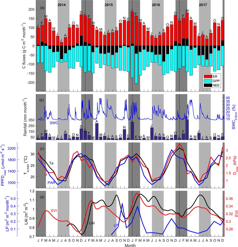
standard deviation of 43 g C m−2 ; Table 1). On average, sum- 3.3 Diurnal trend of CO2 flux and drivers in winter
mer GPP was lower, i.e. more uptake (−400 ± 97 g C m−2 ) and summer
compared to winter GPP (−282 ± 41 g C m−2 ; Table 1), a
difference of ∼ 118 g C m−2 . However, average summer ER The diurnal pattern of NEE in clear-sky conditions differed
was much higher (444 ± 56 g C m−2 ) compared to winter ER between summer and winter (Fig. 2). Relatively speaking,
(159 ± 35 g C m−2 ; Table 1), a difference of ∼ 285 g C m−2 . diurnal NEE was more symmetric in the winter than in sum-
The summer vs. winter ER difference was more than dou- mer. That is, morning and afternoon NEE patterns were mir-
ble the GPP difference; thus, ER had a relatively larger effect ror images and total integrated morning NEE was similar to
over the seasonality of NEE. integrated afternoon NEE during the winter, but strong hys-
teresis occurred in the summer (Fig. 2). This pattern also
translated into hysteresis in the NEE light response curve in
summer, but to a lesser degree in winter (Fig. 3).
Biogeosciences, 15, 3703–3716, 2018 www.biogeosciences.net/15/3703/2018/A. A. Renchon et al.: Upside-down fluxes Down Under 3709
Table 1. Annual precipitation (P , mm yr−1 ), ET (mm yr−1 ), air temperature Ta (◦ C), NEE (g C m−2 yr−1 ), GPP (g C m−2 yr−1 ) and ER
(g C m−2 yr−1 ) for the 4-year study period.
Period P ET Ta NEE GPP ER
(mm yr−1 ) (mm yr−1 ) (◦ C) (g C m−2 yr−1 ) (g C m−2 yr−1 ) (g C m−2 yr−1 )
2014 all 733 797 18 −124 −1301 1177
Winter 149 142 13 −145 −265 120
Spring 129 189 19 −20 −333 313
Summer 279 275 23 80 −302 382
Autumn 176 190 19 −39 −401 362
2015 all 978 938 18 −234 −1517 1283
Winter 122 160 12 −131 −335 204
Spring 237 223 19 −43 −392 349
Summer 273 318 23 24 −426 449
Autumn 345 238 18 −84 −365 280
2016 all 893 852 19 −372 −1664 1292
Winter 335 164 13 −130 −288 158
Spring 96 207 19 −149 −444 295
Summer 412 311 24 −8 −524 516
Autumn 50 171 20 −85 −408 323
2017 all 821 798 19 −171 −1486 1315
Winter 139 148 13 −177 −329 152
Spring 85 178 19 −80 −383 303
Summer 194 236 25 78 −350 428
Autumn 403 237 18 8 −424 432
3.4 Analysis of NEE light response curve 3.5 Atmospheric demand and soil drought control on
GPP, ET, Gs and WUE
The parameters of the NEE light response in summer and
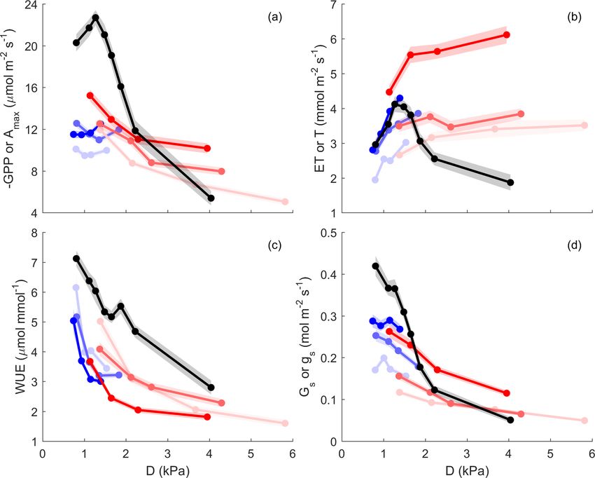
winter are shown in Fig. 4 (see Sect. 2, Eq. 5). The initial We evaluated the effect of SWC and vapour pressure deficit
slope of NEE with light (α) showed no clear dependence on (D) on GPP, ET, water use efficiency (WUE) and surface
Tsoil in winter but exhibited sensitivity during summer, drop- conductance (Gs ) under high radiation (“light-saturated”;
ping precipitously at soil temperature above 23 ◦ C (Fig. 4a). PPFD > 1000 µmol m−2 s−1 ), after filtering periods follow-
α increased with SWC in winter and summer by a factor of ing rain events in order to minimise the contribution of evap-
1.5 (Fig. 4b). In both winter and summer α decreased with D oration to ET (see Sect. 2; Fig. 5). In summer, light-saturated
(D > 1 kPa) and in a similar fashion, approaching a saturating GPP decreased above D ∼ 1.3 kPa, but in winter, GPP did
value of 0.01 (µmol µmol−1 ) at a D of about 2 kPa (Fig. 4c). not vary with D. In summer and in winter, GPP increased
The fitted NEE at saturating light (NEEsat ) was not related to with SWC (Fig. 5a). This is consistent with Fig. 4, where
Tsoil in winter but decreased with increasing Tsoil in summer Rd and NEEsat both increased with SWC. In summer, light-
(Fig. 4d). NEEsat was higher in winter than in summer for a saturated ET increased with D up to ∼ 1.3 kPa, above which
given SWC. The relationship with D was more complicated, it reached a plateau. In winter, ET kept increasing with D,
tending to increase with D in winter, but decreasing with in- as D rarely exceeded 2 kPa. In both seasons, ET increased
creased D in summer, dropping from 9 to 3 µmol m−2 s−1 as with SWC (Fig. 5b). Surface conductance decreased with D
D increased from 1 to 4 kPa. Rd was significantly higher in and SWC especially in summer, indicating strong stomatal
summer than winter across all conditions of Tsoil , SWC and regulation (Fig. 5d). WUE decreased with increasing D in
D (Fig. 4g, h, i). Rd increased with Tsoil in winter and less summer and in winter, because ET increased but −GPP de-
so in summer. In winter, Rd increased up to SWC of 11 %; creased (Fig. 5c).
in summer, Rd was more sensitive to SWC, doubling from
a rate of ∼ 4 to ∼ 8 µmol m−2 s−1 as SWC increased from
about 8 to 20 %.
www.biogeosciences.net/15/3703/2018/ Biogeosciences, 15, 3703–3716, 20183710 A. A. Renchon et al.: Upside-down fluxes Down Under
Figure 2. Diurnal trend (line: median; shade: quartile) of clear-sky-measured NEE (thick black line, µmol m−2 s−1 ); estimated daytime
ecosystem respiration (ER, inferred from a neural network fitted on nighttime NEE, thick dotted red line, µmol m−2 s−1 ); estimated GPP
(inferred as NEE − estimated daytime ER, thick dotted cyan line, µmol m−2 s−1 ); measured vapour pressure deficit (D, thin red line, kPa);
estimated surface conductance (Gs , inferred from Penman–Monteith, blue line, mmol m−2 s−1 ). Grey shade shows night-time (sunset to
sunrise). NEE, GPP and ER number are calculated by integrating the diurnal fluxes as shown in the figure. “Wet” and “dry” soil is defined as
below or above the median of soil water content during summer or winter. Summer is December through February. Winter is June through
August, as defined by the Sydney Bureau Of Meteorology. Colours under NEE rate are shown for visualisation. Note that there is asymmetry
between morning and afternoon NEE in summer, and less so in winter. Note that ecosystem respiration (nighttime NEE) is enhanced by
SWC in summer, and less so in winter. Data used in this figure correspond to clear-sky half-hour values, where high-quality data measured
for NEE were available.
We compared these ecosystem-scale results to the equiv- 3.6 Canopy phenology control of GPP
alent at the leaf scale, which are net photosynthesis at light
saturation Amax (PPFD ∼ 1800 µmol m−2 s−1 ), leaf transpi-
ration T , leaf water use efficiency and stomatal conductance Monthly average photosynthetic capacity (PC) varied by
gs (Fig. 5, black lines). These leaf level measurements are a factor of ∼ 2 across the study period, ranging from
expressed on a leaf-area basis, as compared to ground area 8.4 µmol m−2 s−1 before the leaf flush in November 2014 to
for ecosystem scale. We observed that Amax , T and gs were 15 µmol m−2 s−1 after the leaf flush occurred in March 2016.
more sensitive to D than corresponding ecosystem-scale re- We expected that PC could be predicted by LAI, EVI and
sponses. Amax was much higher than GPPmax at D ∼ 1 kPa, Gs . Leaf area index (LAI) and photosynthetic capacity (PC)
while gs was comparable in magnitude to Gs in the same con- were significantly correlated; the slope was significantly dif-
dition. Leaf transpiration peaked around D = 1.2 kPa, while ferent from zero (r 2 = 0.29, p < 0.005, PC = 8.3 LAI + 3.0,
ET plateaued. Leaf water use efficiency was overall higher Fig. 6). EVI was even more significantly correlated with
than ecosystem WUE. PC (r 2 = 0.46, p < 0.005, PC = 52 EVI − 5.3, Fig. 6). Gs,max
was significantly correlated with PC (r 2 = 0.2, p < 0.005,
Biogeosciences, 15, 3703–3716, 2018 www.biogeosciences.net/15/3703/2018/A. A. Renchon et al.: Upside-down fluxes Down Under 3711
Figure 3. Half-hourly measured NEE vs. PPFD, coloured by Figure 4. NEE µmol m−2 s−1 light response parameters, calculated
D (blue: D < 1.5 kPa; cyan: D of 1.5–3 kPa; red: D > 3 kPa) for for different bins of climatic drivers (soil temperature (Tsoil , ◦ C)
(a) summer and (b) winter periods. Raw data are binned by light at 5 cm depth, soil water content (SWC, %) from 0 to 8 cm depth
levels to show median (lines) and quartiles (white shades) for morn- and atmospheric demand (D, kPa) at 29 m height); only raw, QC-
ing (continuous lines) and afternoon (dotted lines) hours separately. filtered daytime data are used. Light response curve was fitted us-
ing Mitscherlich equation (see Sect. 2); α is the initial slope, near
PPFD = 0 (µmol µmol−1 ); NEEsat µmol m−2 s−1 is NEE at light
PC = 9 Gs,max + 9) and LAI (r 2 = 0.30, p < 0.005, Gs,max = saturation; Rd µmol m−2 s−1 is the dark respiration (NEE when
PPFD = 0). Blue indicates winter months, and red indicates sum-
0.45 LAI − 0.18), and with EVI (r 2 = 0.29, p < 0.005,
mer months. Dots are parameter values for each quartile of driver,
Gs,max = 2.3 EVI − 0.45). The correlations with NDVI were
plotted at x = median of driver for each bin. Shading is 95 % confi-
less significant than with EVI (see Fig. S9). dence interval of the parameter fit.
4 Discussion
low layers sometimes limited decomposition (January and
We measured four consecutive years of carbon, water and en- February 2014, January and December 2015, February and
ergy fluxes in a native evergreen broadleaf eucalyptus forest, December 2017; see Fig. 1), but often regular rainfall main-
including canopy dynamics and environmental drivers (pho- tained adequate soil moisture. The relatively low seasonality
tosynthetically active radiation, air and soil temperature, pre- of GPP may be partly explained by lower photosynthetic ca-
cipitation, soil water content and atmospheric demand). We pacity in early summer (before January) when LAI was at its
hypothesised that the Cumberland Plain forest would be a lowest, and the canopy reached maximum age because new
carbon sink all year-round, similar to other eucalypt forests leaves had not yet emerged. The ER-driven seasonality of
(Beringer et al., 2016; Hinko-Najera et al., 2017; Keith et al., NEE is in sharp contrast with cool-temperate forests where
2012). We also hypothesised higher net carbon uptake during GPP drives the seasonality of NEE. ER-driven NEE season-
summer, due to warmer temperatures, higher light and longer ality was also observed in an Asian tropical rain forest, as
day length contributing to higher photosynthesis, compared ER was higher than GPP in the rainy season leading to net
to winter. However, the site was a net source of carbon during ecosystem carbon loss, while in the dry season, ecosystem
summer, and a net sink of carbon during winter. carbon uptake was positive (Zhang et al., 2010). This pattern
The seasonal pattern of NEE was driven mostly by ER, as was also observed in an Amazon tropical forest (Saleska et
the seasonal amplitude of ER was larger than the seasonal al., 2003).
amplitude of GPP. The seasonality of ER may be explained A strong morning–afternoon hysteresis of NEE response
by the positive effects of higher temperatures on the rates of to PPFD occurred in summer, and less so in winter (Fig. 3).
autotrophic respiration (Tjoelker et al., 2001), and on the ac- In winter, low D and moderately warm daytime air tempera-
tivity of microbes to increase soil organic matter decomposi- tures and high PPFD were sufficient to maintain high photo-
tion (Lloyd and Taylor, 1994); low soil moisture in the shal- synthesis rates throughout most of the day (Fig. 1). In sum-
www.biogeosciences.net/15/3703/2018/ Biogeosciences, 15, 3703–3716, 20183712 A. A. Renchon et al.: Upside-down fluxes Down Under
ecosystem. The similar magnitude for Gs and gs was also
expected, as LAI was close to 1 and Rn was not a driver for
stomatal conductance. The peaked pattern of T versus D, as
opposed to the saturating pattern of ET, may be explained
by (1) the contribution of soil evaporation to ET or (2) the
presence of mistletoe, known for not regulating their stomata
(Griebel et al., 2017). The higher magnitude of leaf water use
efficiency resulted from the combination of higher Amax and
similar or lower leaf transpiration compared to ET. Further-
more, we compared leaf level g1 and ecosystem level G1 , us-
ing the optimal stomatal conductance model (Medlyn et al.,
2011): G1 was lower than g1 (1.6 ± 0.06 for G1 , 4.4 ± 0.2
for g1 ; see Fig. S12).
Our study demonstrated that canopy dynamics (specifi-
cally, LAI in our study) play an important role in regulating
seasonal variations in GPP even in evergreen forests. Similar
observations emerged from a tropical forest, where LAI and
Figure 5. Gross primary productivity or net assimilation (GPP or leaf age explained the seasonal variability of GPP (Wilson
Amax, µmol m−2 (ground or leaf) s−1 ), evapotranspiration or leaf et al., 2001; Wu et al., 2016), as the photosynthetic capac-
transpiration (ET or T , mmol m−2 (ground or leaf) s−1 ), water use ity (PC, the maximum rate of GPP in optimal environmen-
efficiency (WUE = GPP / ET or Amax /T , µmol mmol−1 ) and sur- tal conditions) varied with leaf age. In Australian forests,
face conductance or leaf conductance (Gs or gs , mmol m−2 s−1 ) vs. PC (Amax ) of leaves was also found to decrease with leaf
vapour pressure deficit (D). Leaf level is shown in black; ecosystem age: Amax decreased by 30 % on average between young and
scale is shown in colour (summer in red and winter in blue), at satu- old leaves, for 10 different species (Reich et al., 2009). In
rated PPFD (> 1000 µmol m−2 s−1 ). D is binned into four quartiles
the Cumberland Plain forest, periods with high LAI co-occur
for ecosystem and eight for leaf; Y is mean value for each D bin,
plotted at the median of D bin. Shaded area indicates the standard
with mature, efficient leaves, and periods with low LAI co-
error of the mean. The three colour intensity show SWC quantiles occur with old, less efficient leaves. LAI was correlated with
(SWC < 0.33, SWC (0.33–0.67) and SWC (0.67–1.00) shown in de- PC, which was probably the result of both a greater number
creasing colour intensity). of leaves and more efficient leaves. Remotely sensed vegeta-
tion indices such as EVI or NDVI assess whether the target
being observed contains live green vegetation. In Australia,
mer, two possible explanations of the diurnal hysteresis of NDVI and EVI were good predictors of photosynthetic ca-
NEE include (1) ER is greater in the afternoon compared to pacity in savanna, mulga and Mediterranean–mallee ecosys-
morning and (2) GPP is lower in the afternoon compared to tems (Restrepo-Coupe et al., 2016). For our site, EVI was
morning. Explanation (1) is plausible, as temperature drives a good predictor of PC, which was surprising as satellite-
autotrophic and heterotrophic respiration; however, it is un- derived LAI values have been found to be typically inaccu-
likely to explain the hysteresis magnitude which is higher rate in open forests and forests in southeast Australia (Hill et
in summer compared to winter. Explanation (2) could arise al., 2006). NDVI was a poor predictor of PC (see Fig. S9).
from lower afternoon stomatal conductance or lower photo- In a global study, it was shown that mean annual NEE de-
synthetic capacity (e.g. the maximum rate of carboxylation, creased with increasing dryness index (PET / P ) in sites lo-
Vcmax, decreases at high Ta ), or a combination of both, or cated below 45◦ N (Yi et al., 2010). It has also been shown
even circadian regulation (Jones et al., 1998; Resco de Dios that Eucalyptus grows more slowly in warm environments
et al., 2015). An analysis of surface conductance showed (Prior and Bowman, 2014). At our site, and in a previous
strong stomatal regulation (Figs. 2, 3, 5), induced by high study in eucalyptus forest (van Gorsel et al., 2013), GPP de-
atmospheric demand and high air temperature (Duursma et creased with D above a threshold of ∼ 1.3 kPa. Our results
al., 2014), limiting photosynthesis during the afternoon of indicate that surface conductance (Gs ) decreased above that
warm months (see Fig. S10). These diurnal patterns of NEE, threshold, suggesting that the decrease in GPP is caused by
GPP and ER play a strong role in regulating the seasonal car- stomatal regulation. As D correlates with air temperature, it
bon cycling dynamics in this ecosystem. A wavelet coher- is difficult to distinguish the relative contribution of D and
ence analysis between D and GPP showed strong coherence Ta to the decrease of Gs , but they are both thought to im-
at seasonal timescale (periods of 3 months); see Fig. S11. pact Gs (Duursma et al., 2014). Cumberland Plain has the
We observed comparable responses of leaf-level and highest mean annual temperature and the highest dryness in-
ecosystem-level gas exchange to environmental drivers dex among the four eucalyptus forest eddy covariance sites
(Fig. 5). The larger magnitude of Amax than GPP at low D in southeast Australia (Beringer et al., 2016), which could
may be explained by the proportion of shaded leaves in the
Biogeosciences, 15, 3703–3716, 2018 www.biogeosciences.net/15/3703/2018/A. A. Renchon et al.: Upside-down fluxes Down Under 3713
Figure 6. Relationships between monthly PC (µmol m−2 s−1 ), LAI (m2 m−2 ), enhanced vegetation index (EVI) and maximum surface con-
ductance (Gs,max ). Monthly PC and monthly Gs,max are calculated as the median of half-hourly GPP and half-hourly Gs when PPFD is
800–1200 µmol m−2 s−1 and D is 1–1.5 kPa; rain events are filtered for Gs,max estimation to minimise evaporation contribution to evapo-
transpiration (see Sect. 2). Monthly LAI is calculated as mean of LAI smoothed by a spline. Thick black line shows a linear regression. For
PC calculation, GPP data are only used when quality-checked NEE is available (GPP = NEE measured − ER estimated by a neural network;
see Sect. 2).
explain its strong sensitivity to D and hence its unique sea- The Supplement related to this article is available online
sonality. at https://doi.org/10.5194/bg-15-3703-2018-supplement.
5 Conclusions
The Cumberland Plain forest was a net C source in sum- Author contributions. DT, VRdD, EP, AAR conceived of the
mer and a net C sink in winter, in contrast to other Aus- project; CVMB, CM, EP, AAR, AG, MMB, and DM collected the
data and ran the experiment; AAR, AG, DM, CAW, EP, PI, and
tralian eucalypt forests which were net C sinks year-round.
VRdD analysed the data; AAR and EP wrote the manuscript with
ER drove NEE seasonality, as the seasonal amplitude of ER
input from all other authors.
was greater than GPP. ER was high in the warmer, wet-
ter months of summer, when environmental conditions sup-
ported high autotrophic respiration and heterotrophic de- Competing interests. The authors declare that they have no conflict
composition. Meanwhile, GPP was limited by lower LAI of interest.
and probably older leaves in early summer, and by high
D which limited Gs throughout the summer. Despite being
evergreen, there was significant temporal variation in LAI, Acknowledgements. The Australian Education Investment Fund,
which was correlated with monthly photosynthetic capacity Australian Terrestrial Ecosystem Research Network, Australian
and monthly surface conductance. Understanding LAI dy- Research Council and Hawkesbury Institute for the Environment
namics and its response to precipitation regimes will play a at Western Sydney University supported this work. We thank
key role in climate change feedback. Jason Beringer, Helen Cleugh, Ray Leuning and Eva van Gorsel for
advice and support. Senani Karunaratne provided soil classification
details.
Code and data availability. All the datasets and scripts
used in this manuscript can be downloaded at Edited by: Paul Stoy
https://doi.org/10.5281/zenodo.1219977 (Renchon, 2018). Reviewed by: two anonymous referees
www.biogeosciences.net/15/3703/2018/ Biogeosciences, 15, 3703–3716, 20183714 A. A. Renchon et al.: Upside-down fluxes Down Under
References Foken, T., Wimmer, F., Mauder, M., Thomas, C., and Liebethal,
C.: Some aspects of the energy balance closure problem, Atmos.
Chem. Phys., 6, 4395–4402, https://doi.org/10.5194/acp-6-4395-
Aubinet, M., Chermanne, B., Vandenhaute, M., Longdoz, B., Yer- 2006, 2006.
naux, M., and Laitat, E.: Long term carbon dioxide exchange Gash, J. and Culf, A.: Applying a linear detrend to eddy correlation
above a mixed forest in the Belgian Ardennes, Agr. Forest Mete- data in realtime, Bound.-Lay. Meteorol., 79, 301–306, 1996.
orol., 108, 293–315, 2001. Gimeno, T. E., Crous, K. Y., Cooke, J., O’Grady, A. P., Ósvaldsson,
Aubinet, M., Vesala, T., and Papale, D. (Eds.): Eddy Covariance A., Medlyn, B. E., and Ellsworth, D. S.: Conserved stomatal be-
A Practical Guide to Measurement and Data Analysis, Springer haviour under elevated CO2 and varying water availability in a
Science & Business Media, Dordrecht, the Netherlands, 2012. mature woodland, Funct. Ecol., 30, 700–709, 2016.
Baldocchi, D. D., Ryu, Y., and Keenan, T.: Terrestrial Graham, E. A., Mulkey, S. S., Kitajima, K., Phillips, N. G., and
Carbon Cycle Variability, F1000Research, 5, 2371, Wright, S. J.: Cloud cover limits net CO2 uptake and growth of
https://doi.org/10.12688/f1000research.8962.1, 2016. a rainforest tree during tropical rainy seasons, P. Natl. Acad. Sci.
Baldocchi, D. D., Hicks, B. B., and Meyers, T. P.: Measur- USA, 100, 572–576, 2003.
ing Biosphere-Atmosphere Exchanges Of Biologically Related Griebel, A., Bennett, L. T., Culvenor, D. S., Newnham, G. J., and
Gases With Micrometeorological Methods, Ecology, 69, 1331– Arndt, S. K.: Reliability and limitations of a novel terrestrial laser
1340, 1988. scanner for daily monitoring of forest canopy dynamics, Remote
Barr, A., Richardson, A., Hollinger, D., Papale, D., Arain, M., Sens. Environ., 166, 205–213, 2015.
Black, T., Bohrer, G., Dragoni, D., Fischer, M., and Gu, L.: Use Griebel, A., Watson, D. M., and Pendall, E.: Mistletoe, friend and
of change-point detection for friction–velocity threshold evalua- foe: synthesizing ecosystem implications of mistletoe infection,
tion in eddy-covariance studies, Agr. Forest Meteorol., 171, 31– Environ. Res. Lett., 12, 115012, https://doi.org/10.1088/1748-
45, 2013. 9326/aa8fff, 2017.
Beringer, J., Hutley, L. B., McHugh, I., Arndt, S. K., Campbell, Hill, M. J., Senarath, U., Lee, A., Zeppel, M., Nightingale, J.
D., Cleugh, H. A., Cleverly, J., Resco de Dios, V., Eamus, D., M., Williams, R. D. J., and McVicar, T. R.: Assessment of the
Evans, B., Ewenz, C., Grace, P., Griebel, A., Haverd, V., Hinko- MODIS LAI product for Australian ecosystems, Remote Sens.
Najera, N., Huete, A., Isaac, P., Kanniah, K., Leuning, R., Lid- Environ., 101, 495–518, 2006.
dell, M. J., Macfarlane, C., Meyer, W., Moore, C., Pendall, E., Hinko-Najera, N., Isaac, P., Beringer, J., van Gorsel, E., Ewenz, C.,
Phillips, A., Phillips, R. L., Prober, S. M., Restrepo-Coupe, N., McHugh, I., Exbrayat, J.-F., Livesley, S. J., and Arndt, S. K.: Net
Rutledge, S., Schroder, I., Silberstein, R., Southall, P., Yee, M. ecosystem carbon exchange of a dry temperate eucalypt forest,
S., Tapper, N. J., van Gorsel, E., Vote, C., Walker, J., and Ward- Biogeosciences, 14, 3781–3800, https://doi.org/10.5194/bg-14-
law, T.: An introduction to the Australian and New Zealand 3781-2017, 2017.
flux tower network – OzFlux, Biogeosciences, 13, 5895–5916, Hutyra, L. R., Munger, J. W., Saleska, S. R., Gottlieb, E., Daube, B.
https://doi.org/10.5194/bg-13-5895-2016, 2016. C., Dunn, A. L., Amaral, D. F., De Camargo, P. B., and Wofsy, S.
Breiman, L.: Random forests, Mach. Learn., 45, 5–32, 2001. C.: Seasonal controls on the exchange of carbon and water in an
Didan, K.: MOD13Q1 MODIS/Terra Vegetation Indices 16-Day L3 Amazonian rain forest, J. Geophys. Res.-Biogeo., 112, G03008,
Global 250 m SIN Grid V006, NASA EOSDIS Land Processes https://doi.org/10.1029/2006JG000365, 2007.
DAAC, https://doi.org/10.5067/MODIS/MOD13Q1.006, 2015. Isaac, P., Cleverly, J., McHugh, I., van Gorsel, E., Ewenz,
Dixon, R. K., Brown, S., Houghton, R. E. A., Solomon, A., Trexler, C., and Beringer, J.: OzFlux data: network integration
M., and Wisniewski, J.: Carbon pools and flux of global forest from collection to curation, Biogeosciences, 14, 2903–2928,
ecosystems, Science, 263, 185–189, 1994. https://doi.org/10.5194/bg-14-2903-2017, 2017.
Duursma, R. A., Barton, C. V., Lin, Y.-S., Medlyn, B. E., Eamus, Jones, T. L., Tucker, D. E., and Ort, D. R.: Chilling delays circa-
D., Tissue, D. T., Ellsworth, D. S., and McMurtrie, R. E.: The dian pattern of sucrose phosphate synthase and nitrate reductase
peaked response of transpiration rate to vapour pressure deficit activity in tomato, Plant Physiol., 118, 149–158, 1998.
in field conditions can be explained by the temperature optimum Karan, M., Liddell, M., Prober, S. M., Arndt, S., Beringer, J., Boer,
of photosynthesis, Agr. Forest Meteorol., 189, 2–10, 2014. M., Cleverly, J., Eamus, D., Grace, P., and Van Gorsel, E.: The
Duursma, R. A., Gimeno, T. E., Boer, M. M., Crous, K. Y., Tjoelker, Australian Supersite Network: a continental, long-term terres-
M. G., and Ellsworth, D. S.: Canopy leaf area of a mature ever- trial ecosystem observatory, Sci. Total Environ., 568, 1263–1274,
green Eucalyptus woodland does not respond to elevated atmo- 2016.
spheric CO2 but tracks water availability, Glob. Change Biol., Keeling, C. D., Piper, S. C., Bacastow, R. B., Wahlen, M., Whorf,
22, 1666–1676, 2016. T. P., Heimann, M., and Meijer, H. A.: Atmospheric CO2 and
Fan, S.-M., Wofsy, S. C., Bakwin, P. S., Jacob, D. J., and Fitzjar- 13CO2 exchange with the terrestrial biosphere and oceans from
rald, D. R.: Atmosphere-biosphere exchange of CO2 and O3 in 1978 to 2000: Observations and carbon cycle implications, in:
the central Amazon forest, J. Geophys. Res.-Atmos., 95, 16851– A history of atmospheric CO2 and its effects on plants, animals,
16864, 1990. and ecosystems, Springer, New York, NY, USA, 83–113, 2005.
Foken, T.: The energy balance closure problem: an overview, Ecol. Keith, H., van Gorsel, E., Jacobsen, K. L., and Cleugh, H. A.: Dy-
Appl., 18, 1351–1367, 2008. namics of carbon exchange in a Eucalyptus forest in response to
Foken, T., Gockede, M., Mauder, M., Mahrt, L., Amiro, B., and interacting disturbance factors, Agr. Forest Meteorol., 153, 67–
Munger, W.: Post-field data quality control, Handbook of Mi- 81, 2012.
crometeorology: A Guide for Surface Flux Measurement and
Analysis, 29, 181–208, 2004.
Biogeosciences, 15, 3703–3716, 2018 www.biogeosciences.net/15/3703/2018/A. A. Renchon et al.: Upside-down fluxes Down Under 3715 Knauer, J., Werner, C., and Zaehle, S.: Evaluating stomatal models the southeastern United States, Glob. Change Biol., 21, 827–842, and their atmospheric drought response in a land surface scheme: 2015. A multibiome analysis, J. Geophys. Res.-Biogeo., 120, 1894– Novick, K. A., Ficklin, D. L., Stoy, P. C., Williams, C. A., Bohrer, 1911, 2015. G., Oishi, A. C., Papuga, S. A., Blanken, P. D., Noormets, A., Knauer, J., Zaehle, S., Medlyn, B. E., Reichstein, M., Williams, C. Sulman, B. N., Scott, R. L., Wang, L. X., and Phillips, R. P.: A., Migliavacca, M., De Kauwe, M. G., Werner, C., Keitel, C., The increasing importance of atmospheric demand for ecosystem and Kolari, P.: Towards physiologically meaningful water-use water and carbon fluxes, Nat. Clim. Change, 6, 1023–1027, 2016. efficiency estimates from eddy covariance data, Glob. Change Pan, Y., Birdsey, R. A., Fang, J., Houghton, R., Kauppi, P. E., Kurz, Biol., 24, 694–710, https://doi.org/10.1111/gcb.13893, 2018. W. A., Phillips, O. L., Shvidenko, A., Lewis, S. L., and Canadell, Kolari, P., Lappalainen, H. K., Hänninen, H., and Hari, P.: Relation- J. G.: A large and persistent carbon sink in the world’s forests, ship between temperature and the seasonal course of photosyn- Science, 333, 988–993, 2011. thesis in Scots pine at northern timberline and in southern boreal Pook, E.: Canopy dynamics of Eucalyptus maculata Hook. zone, Tellus B, 59, 542–552, 2007. II. Canopy leaf area balance, Aust. J. Bot., 32, 405–413, 1984. Kormann, R. and Meixner, F. X.: An analytical footprint model for Poulter, B., Frank, D., Ciais, P., Myneni, R. B., Andela, N., Bi, J., non-neutral stratification, Bound.-Lay. Meteorol., 99, 207–224, Broquet, G., Canadell, J. G., Chevallier, F., Liu, Y. Y., Running, 2001. S. W., Sitch, S., and van der Werf, G. R.: Contribution of semi- Lim, P. O., Kim, H. J., and Gil Nam, H.: Leaf senescence, Annu. arid ecosystems to interannual variability of the global carbon Rev. Plant Biol., 58, 115–136, 2007. cycle, Nature, 509, 600–603, 2014. Lindroth, A., Klemedtsson, L., Grelle, A., Weslien, P., and Langvall, Prior, L. D. and Bowman, D. M.: Big eucalypts grow more slowly O.: Measurement of net ecosystem exchange, productivity and in a warm climate: evidence of an interaction between tree size respiration in three spruce forests in Sweden shows unexpectedly and temperature, Glob. Change Biol., 20, 2793–2799, 2014. large soil carbon losses, Biogeochemistry, 89, 43–60, 2008. Reich, P. B., Falster, D. S., Ellsworth, D. S., Wright, I. J., West- Lloyd, J. and Taylor, J. A.: On The Temperature-Dependence Of oby, M., Oleksyn, J., and Lee, T. D.: Controls on declining car- Soil Respiration, Funct. Ecol., 8, 315–323, 1994. bon balance with leaf age among 10 woody species in Australian Medlyn, B. E., Duursma, R. A., Eamus, D., Ellsworth, D. S., Pren- woodland: do leaves have zero daily net carbon balances when tice, I. C., Barton, C. V. M., Crous, K. Y., De Angelis, P., Free- they die?, New Phytol., 183, 153–166, 2009. man, M., and Wingate, L.: Reconciling the optimal and empiri- Renchon, A.: Upside-down fluxes Down Under: CO2 cal approaches to modelling stomatal conductance, Glob. Change net sink in winter and net source in summer in Biol., 17, 2134–2144, 2011. a temperate evergreen broadleaf forest (Version 2), Mitscherlich, E. A.: Das Gesetz des Minimums und das Gesetz des https://doi.org/10.5281/zenodo.1219977, 2018. abnehmenden Bodenertrages, Landw. Jahrb., 38, 537–552, 1909. Resco de Dios, V., Fellows, A. W., Nolan, R. H., Boer, M. M., Moncrieff, J. B., Massheder, J. M., deBruin, H., Elbers, J., Fri- Bradstock, R. A., Domingo, F., and Goulden, M. L.: A semi- borg, T., Heusinkveld, B., Kabat, P., Scott, S., Soegaard, H., and mechanistic model for predicting the moisture content of fine lit- Verhoef, A.: A system to measure surface fluxes of momentum, ter, Agr. Forest Meteorol., 203, 64–73, 2015. sensible heat, water vapour and carbon dioxide, J. Hydrol., 189, Restrepo-Coupe, N., Huete, A., Davies, K., Cleverly, J., Beringer, 589–611, 1997. J., Eamus, D., van Gorsel, E., Hutley, L. B., and Meyer, W. Moncrieff, J. B., Clement, R., Finnigan, J., and Meyers, T.: Av- S.: MODIS vegetation products as proxies of photosynthetic eraging, detrending, and filtering of eddy covariance time se- potential along a gradient of meteorologically and biologically ries, Handbook of micrometeorology, Springer, Dordrecht, the driven ecosystem productivity, Biogeosciences, 13, 5587–5608, Netherlands, 7–31, 2004. https://doi.org/10.5194/bg-13-5587-2016, 2016. Monteith, J. L.: Evaporation and environment, Symposium of the Restrepo-Coupe, N., Levine, N. M., Christoffersen, B. O., Albert, society for experimental biology, the state and movement of wa- L. P., Wu, J., Costa, M. H., Galbraith, D., Imbuzeiro, H., Mar- ter in living organisms, 19, 205–234, Academic Press, New York, tins, G., and Araujo, A. C.: Do dynamic global vegetation models USA, 1965. capture the seasonality of carbon fluxes in the Amazon basin? A Moore, C. E., Brown, T., Keenan, T. F., Duursma, R. A., van Dijk, data-model intercomparison, Glob. Change Biol., 23, 191–208, A. I. J. M., Beringer, J., Culvenor, D., Evans, B., Huete, A., 2017. Hutley, L. B., Maier, S., Restrepo-Coupe, N., Sonnentag, O., Saleska, S. R., Miller, S. D., Matross, D. M., Goulden, M. L., Wofsy, Specht, A., Taylor, J. R., van Gorsel, E., and Liddell, M. J.: Re- S. C., Da Rocha, H. R., De Camargo, P. B., Crill, P., Daube, views and syntheses: Australian vegetation phenology: new in- B. C., and De Freitas, H. C.: Carbon in Amazon forests: unex- sights from satellite remote sensing and digital repeat photogra- pected seasonal fluxes and disturbance-induced losses, Science, phy, Biogeosciences, 13, 5085–5102, https://doi.org/10.5194/bg- 302, 1554–1557, 2003. 13-5085-2016, 2016. Schimel, D. S., House, J. I., Hibbard, K. A., Bousquet, P., Ciais, Munné-Bosch, S. and Alegre, L.: Die and let live: leaf senescence P., Peylin, P., Braswell, B. H., Apps, M. J., Baker, D., and Bon- contributes to plant survival under drought stress, Funct. Plant deau, A.: Recent patterns and mechanisms of carbon exchange Biol., 31, 203–216, 2004. by terrestrial ecosystems, Nature, 414, 169–172, 2001. Novick, K. A., Oishi, A. C., Ward, E. J., Siqueira, M. B. S., Juang, Thom, A.: Momentum, mass and heat exchange of vegetation, Q. J. J. Y., and Stoy, P. C.: On the difference in the net ecosystem Roy. Meteor. Soc., 98, 124–134, 1972. exchange of CO2 between deciduous and evergreen forests in www.biogeosciences.net/15/3703/2018/ Biogeosciences, 15, 3703–3716, 2018
You can also read