WHOI-2021-02 WHOI 260Hz Sound Source - Tuning and Assembly - TECHINCAL REPORT BY
←
→
Page content transcription
If your browser does not render page correctly, please read the page content below
WHOI-2021-02

       WHOI 260Hz Sound Source -
         Tuning and Assembly

                          BY

        James R. Valdes, Heather H. Furey

                      April 2021

              TECHINCAL REPORT

Funding was provided by the National Science Foundation
               under Grant #OCE-1756361

  APPROVED FOR PUBLIC RELEASE; DISTRIBUTION UNLIMITED.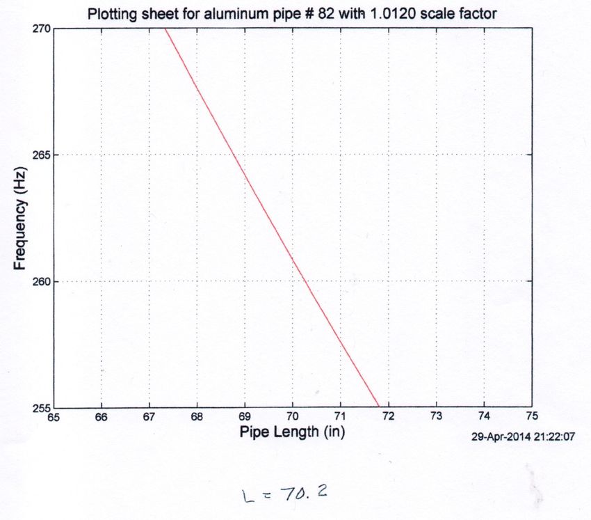
WHOI-2021-02

                 WHOI 260Hz Sound Source - Tuning and Assembly

                                           by

                           James R. Valdes, Heather H. Furey

                         Woods Hole Oceanographic Institution
                          Woods Hole, Massachusetts 02543

                                       April 2021

                                 Technical Report

Funding was provided by the National Science Foundation under Grant No. OCE01756361

    Reproduction in whole or in part is permitted for any purpose of the United States
Government. This report should be cited as Woods Hole Oceanographic Institution Technical
                                 Report, WHOI-2021-02.

                   Approved for public release; distribution unlimited.

                              Approved for Distribution:

                                  Amy Bower, Chair

                         Department of Physical Oceanography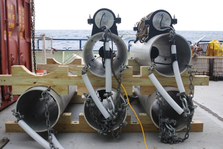
WHOI 260Hz Sound Source – Tuning and Assembly
Furey/Valdes

Table of Contents:
Page           Contents

2              Introduction

5              (1) Test equipment and supplies

7              (2) Resonator tuning

14             (3) Evaluation of in‐situ properties and resonator length

18             (4) Matlab scripts *

27             (5) Electronics test and assembly

34             (6) Pictures *

36             (7) Manual *

50             (8) Electrical Mechanical Documentation

62             (9) Acknowledgements

* These and other items may be downloaded from:
https://www2.whoi.edu/site/bower‐lab/rafosfloats‐soundsources/

1
WHOI Sound Source Testing and Fabrication Notes
Introduction:
Sound sources are designed to provide subsea tracking and re‐location of RAFOS
floats and other Lagrangian drifters listening at 260Hz. More recently sweeps
have been added to support FishChip tracking at 262Hz. These sources must be
tuned to the water properties where they are to be deployed as they have a fairly
narrow bandwidth. The high‐Q resonator’s bandwidth is about 4Hz. This report
documents the tuning, and provides an overview of the sound source assembly.
There are a number of (260Hz) sound source designs available (as of 3/24/2021).
Teledyne Webb Research [TWR] – Reproduces updated Sound Sources
based upon an earlier WHOI (WRC) design.
URI – Pioneered the spherical transducer resonator and a dedicated (now
unavailable) controller.
WHOI – Utilized the URI style resonator with a set of electronics available
from SeaScan. The mechanical design and system integration was
performed at WHOI. This is the current WHOI design.
Develogic Subsea Systems – tunable / fixed frequency source, 200 to 300
Hz.
Those who are interested in a bit of ‘Float History’ should read the Gould (2005)
paper which describes the early float work through the present day Argos
program, or a paper by Rossby (2007) which provides a similar historical overview.
Another interesting paper by Richardson (2005) details some of the early Gulf
Stream work which includes floats.
WHOI Sound source fabrication is comprised of three distinct phases:
1. Ordering the long lead time items in the electronics bill of materials list, and
acquiring the other parts and hardware to assemble the source. Many of
these parts are custom made to the drawings in the Electrical / Mechanical
files.
2. Mechanical resonator ‐ characterization and tuning of the individual
magnetics used in the resonator assembly.
2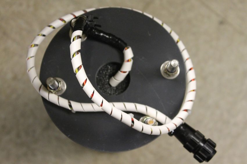
3. Assembly and testing of the sound source electronics, and overall
       integration.

Detailed examples for each step are provided an orderly manner.

The mechanical parts for the electronics need to be fabricated to the drawing files
in the Electrical / Mechanical section of the report. Note that several drawings in
the Source.pdf file have been updated. Please work from the most recent
drawing. In particular, note that the end caps have been modified to use jacking
screws which aid in the disassembly of the pressure housing.

The initial run of sound source electronics was a two board set; a controller and a
signal generator sub‐assembly. In the most recent design SeaScan has integrated
these two assemblies onto a single PC board. They are functionally identical,
testing and mechanical differences are minimal.

There are a number of photos, these may be helpful in identifying components.
These and other items may be downloaded from:
https://www2.whoi.edu/site/bower‐lab/rafosfloats‐soundsources/

************** CAUTION * CAUTION * CAUTION *****************
*                                                                  *
* Sound Sources produce low frequency AC voltages which can        *
* exceed 1000 volts. You may be injured or killed. DO NOT attempt *
* to test or tune the sound source assemblies if you DO NOT have a *
* thorough understanding of the circuitry, generation techniques,  *
* and precautions necessary for personnel safety.                  *
*                                                                  *
************** CAUTION * CAUTION * CAUTION *****************

3
And finally, this report would not be complete without acknowledging the
contributions of Dr. Thomas Rossby. Tom has been the driving force behind
RAFOS and Sound Sources for many years. The resonator described here was
developed by Tom and URI engineer George Schwartze at URI.

References:
Gould, W.J., 2005. From swallow floats to Argo—The development of neutrally buoyant floats. Deep Sea
Research Part II: Topical Studies in Oceanography, 52(3‐4), pp.529‐543. DOI: 10.1016/j.dsr2.2004.12.005

Rossby, T. “Evolution of Lagrangian methods in Oceanography. “ Chapter 1 in Lagrangian Analysis and
Prediction in Coastal and Ocean Processes. Cambridge University Press. 2007

Richardson, P.L., 2005. WHOI and the Gulf Stream. Published in book: Cullen, V., 2005. Down to the sea
for science: 75 years of ocean research, education, and exploration at the Woods Hole Oceanographic
Institution. Woods Hole Oceanographic Institution. https://webarchives.whoi.edu/75th‐
archive/book/whoi‐richardson.pdf

4
Section 1: Test Equipment and Supplies
Pic. 1 – Test Equipment (A)
Shown here are:
Multi‐channel Oscilloscope, 2 to 4 channel
Variable power supply, 15 to 20v @ 1A minimum
Synthesized Function Generator – Stanford Research Systems Model DS345
LCR meter – Wayne Kerr 4234 LCR meter, not essential but useful.
Not shown – Variable power supply, 9 to 15v adjustable, hydrophone and isolated power
supply (battery), miscellaneous wiring, jumpers, and connectors, transducer dummy load,
resonator extension cable.
Pic. 2 – Test equipment (B)
Shown are:
1000v Digital Volt Meters and the custom Test Fixture.
5
Fig.1 – Test Fixture

The fixture utilizes a Maxim – MAX9709 Evaluation kit, this is the same device used in the Sea
Scan class D amplifier assembly. The 9709 is driven externally from the signal generator. The
output of the amplifier is applied to the 9:1 Transformer (Gowanda 70‐0750) and the 1H
inductor (Pulse X‐1149) to drive the resonator at terminals Bk‐Bk. These are the actual
components to be used for each individual Power Amplifier (PA) assembly.

USE CAUTION when working with the fixture as the excitation to the resonator can exceed 1Kv.

Pic. 3 ( a, b, c) – additional test equipment

    a. Dummy Load                 b. YSI, Temperature /           c. Reson hydrophone
                                      Salinity readout        w/interface & power supply

6
Section 2:          Resonator Tuning
The resonator pipe should be prepared as detailed in the RESONATOR drawing. All unused
holes must be PLUGGED with suitable hardware prior to tuning. The ITC‐1007 should be made
ready for installation as shown in Pic. 3. Keep the pins on the transducer / extension cable
shorted at all times when not in use, as high voltages can be induced by the sphere.

Pic. 3   Assembled Transducer, ready for mounting in the resonator.

The transducer assembly must be spliced and made watertight with a urethane (*) potted
connection. See the transducer drawing for details.
The transducer is secured in the STRUT ASSEMBLY with 3/16 inch parachute cord. It is
important that the sphere not be held captive. Initially, the sphere was secured in place with
small turnbuckles – I found that the resonator would not always oscillate when power was
applied. The parachute cord was the initial approach taken by URI, I have found it to function
reliably and to not degrade over the term of deployment. Tip: when the cord is cut, melt the
end to prevent fraying.

It is assumed that the tuning will be at a facility similar to the WHOI outboard dock well in
approximately 60 feet (~20m) of water. The assembled resonator with an extension cable will
be lowered in the dock well to 10m; Take care: if shallower, the assembly is likely to cavitate
when excited at full power.

(*) Urethane – 3M Scotchcast Kit 82‐F1

7
Pic. 5 Resonator support rope (white right ) and hydrophone cable (black left) in the dock
well.
Care should be taken to minimize bubbles on the surface of the resonator prior to tuning.
The assembly may be misted ‐ sprayed with a dilute solution of dish soap from a spray
bottle, prior to lowering into the water. (Not the most effective.)
Soaked for a few hours (overnight) prior to tuning. (Most effective.)
Excited at resonance prior to characterization.
Nominal Resonator Impedance:
LCR check (air) C~84nF, R~10 ohm, (wet) 83nF, 13 ohm [initial values]
Sweep the transducer with the LCR meter to determine the resonate frequency (X=0). Note the
Frequency and the (X) and (R) terms. [Note Freq vs R, i.e., 247.5Hz 555 ohm]
Lower the hydrophone in the dock well to 10m, about 2m from the suspended resonator.
Ready the resonator test fixture for the initial excitation (see Sect.1, Fig.1, Pic 2), set the signal
generator at the {determined} frequency with low drive to minimize output power. Connect the
resonator and observe the power supply current and the resonator output on the scope. Adjust
the drive to limit the current to .5A or less, sweep the generator and note the frequency at
which the ‘sound in the water’ is at a maximum. Sweep the generator to maximize the
observed sound pressure level (SPL). The frequency will likely change as the temperature of the
resonator reaches equilibrium with the water, and the coupling with the water improves as the
bubbles are reduced due to the excitation. When stable, briefly increase the power until the
drive current reaches .9A. Cycle the drive on & off a few times to confirm the reliability of the
transducer at power. Observe the sound in the water with the hydrophone and scope.
NOTE – This is the most likely scenario for a transducer failure, be ready to quickly remove drive
should a failure be observed.
8Allow several hours’ time [overnight is best] for the resonator to stabilize. In the morning again,
check the X & R terms with the LCR meter. R should be ~500 – 600 ohms. The source is tuned in
a ‘broadband’ mode, utilizing the fixture in Section 1, Fig.1, with no inductor and the inductor
terminals shorted. Vref below is the voltage on the transformer secondary.
Following is a transcription from my notebook [Valdes, Sound Source 2013/2014, pg. 88]
Date 4/24/14, Tube #82, Xducer #334, Tube length 73.875”
Time Freq S T Vref Notes
1155 247.9 32.92 8.3 157.4 data point was deleted, not entered into Excel
1202 248.1 32.88 8.4 157.4
1210 248.4 32.93 8.3 157.4
1215 248.3 32.95 8.3 157.3
1242 248.8 33.02 8.4 157.3
LCR 97.9nF, 590 ohm [Reference check]
97.0nF, 600 Ohm
See Section 4 for a description of the Matlab Scripts.
This data is entered into an excel file (data_file_all.xls) and processed using Matlab scripts to
characterize the pipe and to determine the scale factor (SF) for the pipe. With the data stored
in the Excel file run the tune_pipe_v1 Matlab script, use a 1.000 scale factor for your initial
guess. See Dr. Rossby’s description and instructions in Section 4.
Repeat with different scale factors until you have a (relatively) equal distribution of positive and
negative numbers in the f‐diff column.
Output from Matlab tune_pipe_v1 script:
>> tune_pipe_v1
Enter pipe #82
Enter scale factor: 1.0
ans =
scale factor = 1.0000
year mon day pipe lngh f‐obs f‐exp f‐diff s‐vel
2014 4 24 82 73.9 248.1 251.3 ‐3.2 1481.4
2014 4 24 82 73.9 248.4 251.2 ‐2.8 1481.1
2014 4 24 82 73.9 248.3 251.2 ‐2.9 1481.2
2014 4 24 82 73.9 248.8 251.3 ‐2.5 1481.6
Note : SF yields all negative f-diff results
>> tune_pipe_v1
Enter pipe #82
Enter scale factor: 1.01
9ans = scale factor = 1.0100 year mon day pipe lngh f‐obs f‐exp f‐diff s‐vel 2014 4 24 82 73.9 248.1 248.8 ‐0.7 1481.4 2014 4 24 82 73.9 248.4 248.7 ‐0.3 1481.1 2014 4 24 82 73.9 248.3 248.7 ‐0.4 1481.2 2014 4 24 82 73.9 248.8 248.8 0.0 1481.6 Note: non-even f-diff distribution with the given SF >> tune_pipe_v1 Enter pipe #82 Enter scale factor: 1.02 ans = scale factor = 1.0200 year mon day pipe lngh f‐obs f‐exp f‐diff s‐vel 2014 4 24 82 73.9 248.1 246.3 1.8 1481.4 2014 4 24 82 73.9 248.4 246.3 2.1 1481.1 2014 4 24 82 73.9 248.3 246.3 2.0 1481.2 2014 4 24 82 73.9 248.8 246.3 2.5 1481.6 Note: SF yields all positive f-diff values >> tune_pipe_v1 Enter pipe #82 Enter scale factor: 1.015 ans = scale factor = 1.0150 year mon day pipe lngh f‐obs f‐exp f‐diff s‐vel 2014 4 24 82 73.9 248.1 247.6 0.5 1481.4 2014 4 24 82 73.9 248.4 247.5 0.9 1481.1 2014 4 24 82 73.9 248.3 247.5 0.8 1481.2 2014 4 24 82 73.9 248.8 247.6 1.2 1481.6 Note: f-diff still all positive >> tune_pipe_v1 Enter pipe #82 Enter scale factor: 1.012 ans = scale factor = 1.0120 year mon day pipe lngh f‐obs f‐exp f‐diff s‐vel 2014 4 24 82 73.9 248.1 248.3 ‐0.2 1481.4 2014 4 24 82 73.9 248.4 248.3 0.1 1481.1 10
2014 4 24 82 73.9           248.3 248.3   0.0 1481.2
2014 4 24 82 73.9           248.8 248.3   0.5 1481.6

Note: Much better distribution

>> tune_pipe_v1
Enter pipe #82
Enter scale factor: 1.011

ans =

scale factor = 1.0110

year mon day pipe lngh f‐obs f‐exp         f‐diff s‐vel
2014 4 24 82 73.9 248.1 248.5             ‐0.4 1481.4
2014 4 24 82 73.9 248.4 248.5             ‐0.1 1481.1
2014 4 24 82 73.9 248.3 248.5             ‐0.2 1481.2
2014 4 24 82 73.9 248.8 248.5              0.3 1481.6
>>

After reviewing the results a SF = 1.012 was chosen.

Note, I have not observed a SF less than 1 to date.

Once the tube has been characterized, it can be tuned to the specific water mass, or retuned to
a different set of in‐situ values.

Adding the tuning parameters under notes is helpful for future reference.

11
Excel – data_file_all example:

12
13
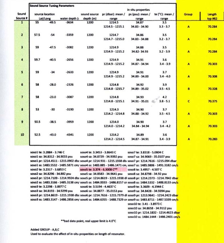
Section 3: Evaluation of In‐Situ Properties
                                    & Resonator Length

Example file : OSNAP_SoundSource Tuning‐1A.xlsx [OSNAP experiment]

Note: For Tuning purposes we are only interested in the data contained in columns C thru J in
Table 1, as these describe the In‐Situ water properties where the sources will be deployed.
Columns K and L were added to the original spreadsheet, after reviewing and grouping the
data.

From the OSNAP report, 4/30/2014.
Sound source tuning parameters – reference OSNAP_SoundSourceTuning‐1A.xls
Group (ABC) sound sources by in‐situ parameters (T), for SS1 evaluate effect on calculated tube
length for the variations in T & S. [ Example tube #82 is used for all calculations / evaluations.]

Source         Sal            Temp            Press          Length (tube #82)

1,2,3          34.870         3.500           1200           70.284
1A1            34.830         3.300           1200           70.246
1A2            34.830         3.700           1200           70.316
1A3            34.900         3.300           1200           70.258
1A4            34.900         3.700           1200           70.306

4B             34.91          3.600           1200           70.303
5B             34.91          3.700           1200           70.308
6B             34.92          3.900           1200           70.328
7C             34.93          4.200           1200           70.375
8,9B           34.90          3.700           1200           70.303
10B            34.89          6.600           1200           70.283

Other useful constants … ~3.33 Hz/inch of tube, assume the tube trim is accurate to .1 inch.
Length (limits) = 70.284 – 70.375, Average length = 70.305
Suggests we might use the in‐situ values for Source 4 and the individual Scale Factors for each
tube as the basis for tuning. The evaluation summary is shown in columns K & L.

14
Using Tube 82 as an example, from
The raw date is entered into the excel file [data_file_all.xls]
Inner Wall temper
Pipe Met Length(in dia(in thkns salinity(PS ature(° depth snd resonanc meth
# al Year Month Day ) ) (in) U) C) (m) vel e(Hz) od where
82 Al 2014 4 24 73.87 15 0.5 32.88 8.4 10 248.1 0 whoi
82 Al 2014 4 24 73.87 15 0.5 32.93 8.3 10 248.4 0 whoi
SF
82 Al 2014 4 24 73.87 15 0.5 32.95 8.3 10 248.3 0 whoi 1.012
82 Al 2014 4 24 73.87 15 0.5 33.02 8.4 10 248.4 0 whoi
open
82 Al 2014 5 2 70.3 15 0.5 33.2 8.8 10 264.3 0 whoi …
82 Al 2014 5 2 70.3 15 0.5 33.3 8.8 10 265.1 0 whoi ….
82 Al 2014 5 2 70.3 15 0.5 33.34 8.9 10 265.5 0 whoi .holes
plugged
82 Al 2014 5 2 70.3 15 0.5 33.38 8.9 10 257.4 0 whoi ---
82 Al 2014 5 2 70.3 15 0.5 33.45 8.9 10 259.6 0 whoi ….
….
82 Al 2014 5 2 70.3 15 0.5 33.45 8.9 10 260.1 0 whoi holes
Data in RED used for tuning. Blue lines were after trimming with mounting holes open, results
were inconsistent – frequency much higher than expected. Black data is with holes plugged.
Output from tune_pipe_v1.m after adjusting the scale factor for the empirical fit.
>> tune_pipe_v1
Enter pipe #82
Enter scale factor: 1.012
ans = scale factor = 1.0120
year mon day pipe lngh f‐obs f‐exp f‐diff s‐vel
2014 4 24 82 73.9 248.1 248.3 ‐0.2 1481.4
2014 4 24 82 73.9 248.4 248.3 0.1 1481.1
2014 4 24 82 73.9 248.3 248.3 0.0 1481.2
2014 4 24 82 73.9 248.4 248.3 0.1 1481.6
The tune_pipe_v1.m script is only used to determine the scale factor (SF) to be applied to the
pipe. The actual length in‐situ is determined from resonance_fcnof_length.m script, the
resulting plot is used to determine the length of the pipe. Actual length from the plot at 260Hz
was determined using a set of dividers to be 70.2 in.
15The final OSNAP results obtained after tuning is summarized below. All resonators are tuned to 4B parameters; S=34.91, T=3.6, P=1200. Tube S.F Length Tube S.F Length 80 1.015 70.0 86 1.0135 70.25 81 1.013 70.2 87 1.015 70.0 82 1.012 70.2 88 1.009 70.5 83 1.013 70.2 21 1.012 70.3 84 1.016 70.0 24 1.012 70.3 85 1.012 70.3 16
Table 1: OSNAP_SoundSource Tuning‐1A.xlsx

         C     D       E       F        G          H            I           J          K          L

Table 1: In situ properties derived from historical Argo data for locations where sound sources will be
moored. Tuning for each sound source is specific to the water properties at the site of deployment.

17
Section 4: URI Matlab Scripts (Dr. T. Rossby)
A note on the use of the pipe tuning programs,
October 10, 2005.
(minor update May 25, 2011)
(delete all earlier notes on pipe tuning)
The program tune_pipe_v1.m is an evolution of earlier programs. It combines the steel and
aluminum versions into one, and it requires that all information be supplied in an excel -file
called data_file_all.xls These steps greatly simplify use and increase robustness. Above all, the
use of excel to enter the data removes a number of earlier headaches reading ascii files. Use of
the program tune_pipe_v1.m is an iterative process that might be automated at a future time, but
for now I think it best to examine closely the numbers before making a decision.
The objective of tune_pipe_v1.m is one and one only, namely to determine how this pipe
deviates from the ideal pipe of the same dimensions. These deviations can occur because of non-
uniformities in pipe dimensions or properties. The program requires for this purpose tuning data,
that is a determination of frequency of resonance in water of known properties. The data from
each tuning are entered into the above excel file. Because each measurement has some error or
uncertainty associated with it (we still need to better understand how to reduce this measurement
uncertainty), it is important to determine resonance more than once, preferably three times in
case the results differ.
Operation of tune_pipe_v1.m is very simple. After entering pipe number, you enter a first guess
for the scale factor (start with 1.0 if nothing else). The program will show a table of observed and
expected resonance frequencies. (I have kept the plot for historical reasons, but it serves no
useful purpose now.) If the expected frequencies are too low (differences are negative), increase
the scale factor somewhat (try increasing by 1% to 1.01) and rerun with the new value. When
you have obtained a result where the differences scatter comparably to positive and negative
values you can decide this is the best estimate for the scale factor. By doing this manually, you
can inspect the results as you go along. Very importantly, you can decide to ignore outliers and
focus on data that cluster tightly (kind of like choosing the median value). In summary, the key
result of the first program is making a best estimate of the scale factor. It is a number close to
one, but the significance lies in the third decimal. This number essentially encapsulates the
particular properties of the pipe. It matters because the mechanical q-factor of the pipes that
resonance must be determined for each pipe separately. But once this scale factor has been
determined, it can be used to predict the frequency of resonance in situ, i.e. in waters where it is
to be used. This is what the second program, resonance_fcnof_length.m is used for.
18This program, resonance_length.m, is used to predict the frequency of resonance as a function of pipe length given the in-situ water properties and the previously determined scale factor. The output is a plot of resonance as a function of pipe length. When operating resonance_fcnof_length.m be sure to enter the numbers inside square brackets [nnn mmm] with space between entries, not commas. The format of the excel file is self-evident, but is indicated here: A: pipe # B: material (should be Al for aluminum and Fe for steel) C: year D: month E: day F: pipe length (inches) G: pipe inner diameter (inches) H: pipe wall thickness (inches) I: salinity at time of this tuning (PSU) J: temperature at time of this tuning (°C) K: water depth at time of tuning (m) L: speed of sound (m/s); no longer needed as it is computed by program M: measured frequency of resonance (Hz) N: type of tuning (0 = voltage method expected; 1 = tuned circuit used in early days) O: misc info such as location or state of tide Editor Note: Some of the scripts could use a ‘tidy up’; Removing links which are no longer required, etc. The resonator count has been modified to allow greater than 100. The M file scripts are available at: https://www2.whoi.edu/site/bower-lab/rafosfloats-soundsources/ 19
Matlab code courtesy of Dr. Thomas Rossby
% tune_pipe_v1.m
%
% Estimating pipe cavity resonance frequency.
% We consider a simple pipe of:
%
%   L = length [m]
%   d = inside diameter [m]
%   a = inside radius [m]
%   t = wall thickness [m]
%   E = Young's modulus [Pa]
%   K = bulk modulus of fluid [Pa]
%   c = speed of sound in fluid [m/s]
%
% In the model the monopole driver is 'transparent' (no physical presence).
% The scale factor can be adjusted to fit the pipe as closely as possible
% such that the plot can be read directly, i.e. given a frequency
% and speed of sound the required pipe length can be read directly.
%
% This package evolves from earlier pipe_tune code. This version estimates
% K as a function of target water properties.
% ---------------------------------------------------------------------
clear all
mpi = 0.0254 ;                      % meters per inch (inches to meters).
K    = 2.28e9 ;                     % bulk modulus of seawater - used only
                                    % to set up plot; it is **NOT** used
                                    % for pipe tune calculations
% ---------------------------------------------------------------------------
-
% -- read in pipe information

% -- Note that the data_file.txt columns are:
%    Pipe metal YYYY MM DD pipe_length pipe_ID wall_thickness
%    Sal   Temp   Press Svel Freq driver      Comment/location

%      Under driver enter 0 for voltage driver or 1 for tuned (coil) driver

[A,B] = xlsread('data_file_all.xls');

% delete top row in B (don't know how to rid it in EXCEL had header info
% now moved to bottom)
B = B(2:end,:);
Pnbr = A(:,1); Mtl = B(:,2); year = A(:,3); month = A(:,4); day = A(:,5);
pipelen = A(:,6);
ID = A(:,7); TK = A(:,8); S = A(:,9); T = A(:,10); Pr = A(:,11); svel =
A(:,12);
freq = A(:,13); Drvr = A(:,14); whre = B(:,15);

%    Enter which pipe to analyse:
%    specify pipe # - for consistency assumes voltage drive mode (Drvr == 0).
P    = input('Enter pipe #');
J    = find(Pnbr == P & Drvr == 0);

% determine properties of pipe (must be Al or Fe at present):

20
mtrl = Mtl(J(1));
if strcmp(mtrl,'Al')
E = 7.0e10; % -- Young's modulus (aluminum)
matrl = 'aluminum';
elseif strcmp(mtrl,'Fe')
E = 1.95e11 ; % -- Young's modulus (304SS)
matrl = 'steel';
else
disp('check material type')
return
end
% get radius and wall thickness:
id = ID(J); tk = TK(J);
id = unique(id(~isnan(id))); % get ID from list (need only scalar
since always the same)
tk = unique(tk(~isnan(tk))); % likewise for wall thickness
d = id*mpi; % inner diameter of pipe (units are
metric here)
a = d/2; % inner radius of pipe
t = tk*mpi; % wall thickness
% Now determine resonant frequency as a function of
% sound velocity and pipelength
%%%%%%%%%%%%%%%%%%%%%%%%%%%%%%%%%%%%%%%%%%%%%%%%%%
% This section is highlighted because this
% is where the scale factor is tweaked to
% minimize the difference between expected and
% measured frequency (Hz). Typically a couple
% of % less than unity. If differences > 0,
% reduce scf slightly.
% Set scf = 1 if no empirical adjustment wanted
% Enter scale factor:
scf = input('Enter scale factor: ');
%%%%%%%%%%%%%%%%%%%%%%%%%%%%%%%%%%%%%%%%%%%%%%%%%%
% PLOT parameters are set here:
% Range of speeds of sound in m/s for plot (x-axis):
sv = sw_sspd(S(J),T(J),Pr(J));
xmin = min(sv); % min sound velocity
xmax = max(sv); % max sound velocity
sl = 1400:10:1550;
L = sl < xmin;
xmin = max(sl(L)); % have lower plot limit given sound
velocities
L = sl > xmax;
xmax = min(sl(L)); % have upper plot limit given sound
velocities
% Range of pipe lengths in inches for plot (y-axis):
ymin = min(pipelen(J)); % min pipe length
21ymax = max(pipelen(J)); % max pipe length
pl = 40:5:90;
L = pl < ymin;
ymin = max(pl(L)); % have lower plot limit given pipelengths
L = pl > ymax;
ymax = min(pl(L)); % have upper plot limit given pipelengths
ystep = 2;
L = ymin:ymax ; % range of pipe length in inches
LE = (L/2)*mpi + 0.6*a ; % effective length (includes end-effect)
LE = LE*scf ;
C = xmin:xmax ;
CE = C / sqrt( 1+K*d/(E*t) ) ; % -- effective speed of sound in pipe
[Xe,Ye] = meshgrid(CE,LE) ;
F = ( 1*Xe )./( 4*Ye ) ;
[X,Y] = meshgrid(C,L) ;
% -----------
% Set up plot
figure(1)
clf
orient portrait
plotdef
axes( 'Position', [ 0.15 0.4 0.75 0.5] )
% plot isopleths of resonant frequencies based on a mean seawater bulk
modulus:
[ cont, hc ] = contour( C, L, F, [190:1:290], 'k' ) ;
set( hc, LW, [0.01] )
hold on
[ cont, hc ] = contour( C, L, F, [200:5:300], 'k' ) ;
set( hc, LW, [2.0] )
clabel( cont, hc )
axis([xmin xmax ymin ymax]) % set plot limits
% get data lines. Allow for several entries with same pipe length.
lines = pipelen(J);
nlines = length(lines) ;
colors = 'brcmk' ; % colors for different pipe lengths
for j = 1:nlines
k = J(j);
len = pipelen(k);
sv = sw_sspd(S(k),T(k),Pr(k)); % speed of sound for this case (m/s)
plot( [ xmin xmax ], [ len len ], colors(rem(j,5)+1) ) ;
plot( sv, len, 'w.', MS, [48] ) ;
bm = sw_seck(S(k),T(k),Pr(k))*1e5; % bulk modulus for this case (Pa)
Fres(j) = (sv/(sqrt(1 + bm*d/(E*t))))/((len/2*mpi + 0.6*a)*scf)/4;
df(j) = freq(k) - Fres(j);
index = min(find( lines == len ));
plot( sv, len, sprintf( '%so', colors(rem(index,5)+1) ), MS, [16] ) ;
text( sv, len, sprintf( '%2d\n%5.1f', Pnbr(k), freq(k) ), ...
FS, 5, HA, 'center' )
22str(j,1:66) = sprintf(' %2d %2d %2d %2d %4.1f %5.1f %5.1f
%5.1f %5.1f', ...
year(k), month(k), day(k), Pnbr(k), len, freq(k), Fres(j), df(j),
sv);
end
hold off
xlabel( 'Sound Velocity (m/s)', FS, [14], VA, 'top' )
ylabel( 'Pipe Length (in)', FS, [14], VA, 'bottom' )
title(sprintf('Plotting sheet for %s pipe # %d with %5.3f scale factor',
matrl, P, scf), FS, [14] )
grid on
% ------------------------------
% Tabulate results below figure:
hdr = sprintf(' year mon day pipe lngh f-obs f-exp f-diff s-
vel');
axes( 'Position', [ 0.15 0.05 0.75 0.3] )
axis off
warning = 'PLOT FOR DISPLAY ONLY, DO NOT USE TO ESTIMATE PIPE LENGTH';
text(0.1,0.9,warning, FS, 10, HA, 'left')
text(0.0,0.8,hdr, FS, 10, HA, 'left',FN, 'monaco')
text(0.0,0.6,str, FS, 10, HA, 'left',FN, 'monaco')
sprintf('scale factor = %6.4f',scf)
disp(hdr)
disp(str)
putdate
HA = 'HorizontalAlignment' ;
VA = 'VerticalAlignment' ;
IP = 'Interpreter' ;
FS = 'FontSize' ;
MS = 'MarkerSize' ;
LW = 'LineWidth' ;
FN = 'FontName' ;
23Matlab code courtesy of Dr. Thomas Rossby
% resonance_fcnof_length
% This program plots frequency of resonance for a given pipe type as a
% function of pipe length and for desired or expected water
properties.
% After entering pipe #, it will ask for water properties.
% This program will probably get appended into the pipe-tune program.
% read in excel file of pipe data.
clear all
clf
[A,B] = xlsread('data_file_all.xls');
B = B(2:end,:);
Pnbr = A(:,1); Mtl = B(:,2); year = A(:,3); month = A(:,4); day =
A(:,5); pipelen = A(:,6);
ID = A(:,7); TK = A(:,8); S = A(:,9); T = A(:,10); Pr = A(:,11); svel
= A(:,12);
freq = A(:,13); Drvr = A(:,14); whre = B(:,15);
% Enter which pipe to analyse:
% specify pipe # - for consistency assumes voltage drive mode (Drvr ==
0).
NN = input('Enter pipe # and scale factor in brackets [n1 n2]:');
P = NN(1)
scf = NN(2)
J = find(Pnbr == P & Drvr == 0);
% determine properties of pipe (must be Al or Fe at present):
mtrl = Mtl(J(1));
if strcmp(mtrl,'Al')
E = 7.0e10; % -- Young's modulus (aluminum)
matrl = 'aluminum';
elseif strcmp(mtrl,'Fe')
E = 1.95e11 ; % -- Young's modulus (304SS)
matrl = 'steel';
else
disp('check material type')
return
end
% get radius and wall thickness:
mpi = 0.0254 ; % meters per inch (inches to
meters)
id = ID(J); tk = TK(J);
id = unique(id(~isnan(id))); % get ID from list (need only
scalar since always the same)
tk = unique(tk(~isnan(tk))); % likewise for wall thickness
24d = id*mpi; % inner diameter of pipe (units
are metric here)
a = d/2; % inner radius of pipe
t = tk*mpi; % wall thickness
disp('Next, enter the properties of water where the pipe will
operate')
disp('in the format [S T P]')
wtr = input('>');
S = wtr(1);
T = wtr(2);
Pr = wtr(3);
C = sw_sspd(S,T,Pr); % speed of sound in m/s for this
water
K = sw_seck(S,T,Pr)*1e5; % bulk modulus in Pa for this
water
ymin = 60; ymax = 80;
L = ymin:ymax ; % set a range of pipe lengths in
inches
LE = (L/2)*mpi + 0.6*a ; % effective length (includes end-
effect)
%%%%%%%%%%%%%%%%%%%%%%%%%%%%%%%%%%%%%%%%%%%%%%%%%%
% The scale factor must be entered here. It is determined by
minimizing the
% scatter between observed and estimated resonance frequencies in
program
% tune_pipe_v?.m The value of scf so obtained is entered here
(eventually)
% it will be entered at the command line.
% scf = .992;
%%%%%%%%%%%%%%%%%%%%%%%%%%%%%%%%%%%%%%%%%%%%%%%%%%
LE = LE*scf ;
CE = C / sqrt( 1+K*d/(E*t) ) ; % -- effective speed of sound in
pipe
F = CE./(4*LE);
K
sprintf('scale factor = %6.4f',scf)
figure(2)
clf
plot(L,F,'r')
axis([65 75 255 270])
grid
xlabel( 'Pipe Length (in)','FontSize', [14])
ylabel( 'Frequency (Hz)','FontSize', [14])
title(sprintf('Plotting sheet for %s pipe # %d with %5.4f scale
factor', matrl, P, scf),'FontSize', [14] )
25text(ymin+0.5,min(F)+1,sprintf('Target water properties for this plot
are: %5.2fPSU %5.2fC %5.0fdbars',S,T,Pr))
putdate
26Section 5: Sound Source Electronics Test & Assembly It is assumed that the operator has a basic understanding of the instrument and electronics. The description which follows is an overview ‐ not a step‐by‐step tutorial. Initial testing utilizes the test fixture with the internal power amplifier and the actual transformer and inductor assembled on the bench, breadboard fashion. Verify that full power can be achieved using the dummy load (Sect.1, Pic.3a) in place of the resonator (Xducer) as shown (Sect.1, Fig.1). This is the same set‐up used for tuning the resonator with the addition of the 1H inductor. Again, USE CAUTION – The voltage on the output of the inductor can exceed 1000 VOLTS. If necessary the gain of the amplifier can be adjusted with the jumpers on the circuit board. They are located in a row between the two capacitors. These are generally preset by SeaScan. The parameters of interest during testing are given on pg. 6, Fig 1 [, Source_Test]. When tuning in‐water, a hydrophone placed about 20m away at 10m depth is used with an oscilloscope (‘scope’) to monitor the source for cavitation. The source is lowered to a depth of 10 meters and gently excited to reduce the air bubbles on the resonator tube. Given local conditions the tube may not be resonant at the desired in‐situ properties. The bubbles may 27
also have an effect on the resonant frequency so sweeping the excitation frequency may be
helpful. At this point there are two resonances; the mechanical resonance of the tube and the
electrical resonance of the L/C circuit. You can check the mechanical resonance by driving the
transducer in the ‘Broadband’ mode w/o the inductor as was done during the initial tuning.
From a practical point of view, I find tuning in Woods Hole off the dock to be best in the early
spring (March‐May) when the local water is cold. In the cold water the resonance is close to
260Hz for the resonator. It’s generally best to let the source soak at depth for a few hours to
de‐bubble before tuning. Always bring up power slowly ‐ the output from the inductor can have
1000v at full output, across the cable connecting it to the resonator.

Be ready to remove the 21v supply at the first indication of a problem.

The first step is to tune the magnetics; the inductor and transducer capacitance are treated as a
series tuned circuit. The inductor is a split core with .010 inch shims on each side. The number
of shims is changed to increase or decrease the inductance to achieve resonance. What is
resonance?

There are a number of ways to describe resonance. (Series R L C Circuit)
       * When XL=Xc,
       * The frequency at which the Rs term is maximum (XL cancels Xc),
       * The frequency at which the Voltage and Current are in phase,
       * The frequency of maximum Power Transfer (output).

Beware of ‘ground loops’; I have not had a problem but you might consider using an isolation
transformer with the test equipment that require AC power. Tuning is a bit subjective, it takes
some time to develop a ‘feel’. I’m attempting to quantify the process but it is not exact. Using
the Test Fixture you can easily monitor the phase between the voltage and the current with a
scope.

Scope Ch 1 – Voltage, connect a probe across the transformer secondary. (trigger here)
     Ch2 – Current, connect a probe across the 10 Ohm resistor

In both cases the ‘low side’ of the secondary is the ground reference for the scope.

Again, gently apply excitation and observe the waveforms. I find the phase to be somewhat
dynamic, it seems to vary with the power applied. Since the sweeps (RAFOS, 1.523hz, and the
Fish Chip, 3 Hz) are fairly narrowband I tend to move the resonance point away from F0, where
the phase changes. Which side doesn’t matter it depends upon the available shims.

28
Some of us old‐timers in EE may recall; “ELI the ICE” man. (From GOOGLE) ELI the ICE man is an
old memory "crutch" to help one remember the A.C. current and voltage phase angle
relationship in inductors and capacitors.
ELI tells us that the voltage (E) leads or comes before current (I) in an inductor (L).
ICE tells us the current (I) leads or comes first before voltage (E) in a capacitor (C).
Here are a few examples for reference:
Current leading Voltage leading ‘In Phase’, Voltage 1.9 deg leading
Adjusting the inductance is accomplished by varying the number of shims between the two half
sections of the core. I generally use a band clamp to apply pressure and to keep the cores in
place. Typically I grasp the cores to apply pressure when tuning. Keep in mind the working
voltage and use care when handling.
After tuning ‘serialize’ the Inductors to the resonator, as they are not interchangeable.
Electronics Mechanical assembly:
The end cap can be assembled with the external connectors and standoffs. The upper section
two plates, backplane plate, and separator rods can also be assembled. Do not complete the
assembly until the tuned inductors are available. Refer to the pictures folder for mounting and
placement details. The electronics are mounted to the damper mounts on the plate. The
transformer can now be mounted and the upper assembly wired, see the sound source
interconnection diagram.
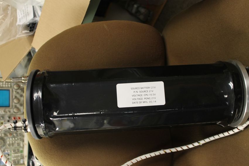
29The inductor is secured to the plate with multiple sections of double sided foam adhesive. It is also secured with tie wraps. The two sections can now be fitted together and made ready for testing. See the SS_Test file for interconnection and testing recommendations. Battery Pack: Add the spline wrap and secure the wires to one of the mounting rods to provide protection and strain relief. 30
The pack is assembled with tie rods, tighten to secure the pack, DO NOT OVERTIGHTEN.

31
The battery is assembled and secured to the snap ring.

Again, I suggest that you browse the pictures for details.

32
Bill of Materials: Components needed for sound source electronics fabrication.

33
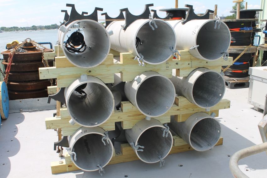
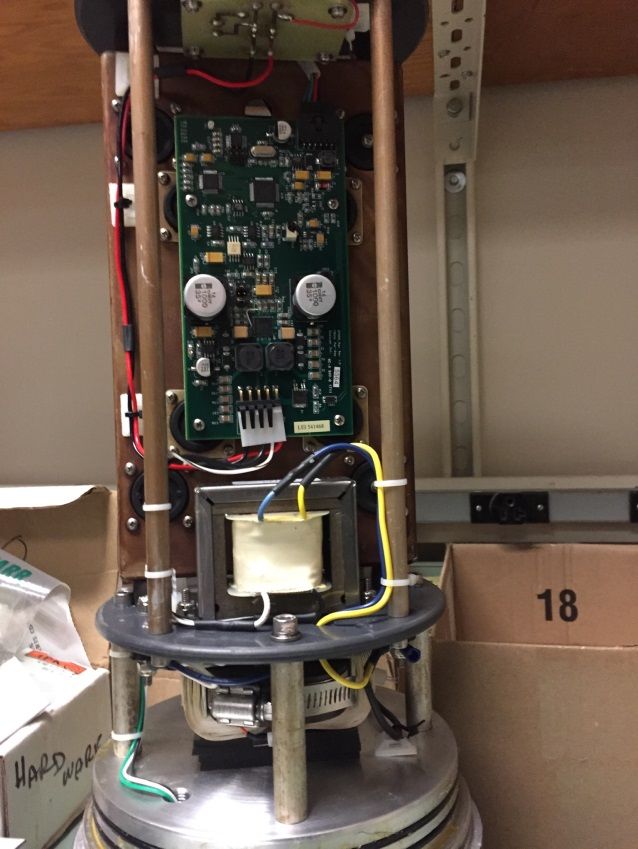
Section 6: Sound Source Pictures

Sound source photographs of the electronics during fabrication and assembly.

Many source photographs are available at: https://www2.whoi.edu/site/bower‐lab/rafosfloats‐
soundsources/

34
35
Section 7

     WHOI Sound Source
       Manual V1.1

            May 2018
            J. Valdes

36
WHOI Sound Source Manual V1.1
Warnings:
Risk of Explosive Gas – Sound sources contain a large volume of alkaline batteries
in a sealed pressure housing. Upon discharge alkaline batteries are known to
release a small quantity of explosive gasses. Use care and due‐diligence when
handling sealed pressure housings.
High Voltage present – The output of the amplifier is on the order of 1000v RMS.
Disassembly of the source is only to be undertaken by trained and qualified
personnel.
To minimize these risks we recommend the following:
Leave the interior of the case at atmospheric pressure. Install the vacuum
plug on the lower end cap and evacuate prior to deployment.
Once sealed, monitor the interior pressure (vacuum) via the external
communications link.
Remove any possible sources of ignition (sparks, flame, etc.) from the
vicinity of the sound source.
Never operate the sound source without a resonator or dummy load attached.
Observe the Pmax limitation and limit the source to two pongs on deck when
in the Run Mode. Note; the source starts at level 02 and ramps up with each
successive pong to the level of Pmax.
General Information:
In this discussion some knowledge of the RAFOS system is assumed.
The WHOI sound source is intended to facilitate acoustic tracking of subsurface
instrumentation, i.e., profiling instruments, RAFOS floats, gliders, etc. The sound source emits a
unique swept frequency acoustic signal referred to as a “pong”. The pong is generally at a low
frequency (Description / Specifications: Resonator: Aluminum Length: 71”, OD : ~ 1.8m, Weight, ~81 Kg (air), 52 Kg (water) Spherical Projector, Channel Technologies Group, ITC‐1007 Electronics pressure case (includes end caps) Length, ~1.3m x 2.95cm, 50” x 7.5 “ Weight, ~ 54Kg, 120 lb. Main battery, 21v x 10 stacks (D‐cells), 10.5v x 3 stacks (D‐cells) Source Electronics, Sea Scan sound source module Source is intended to be deployed ‘in‐line’ with the mooring. There are 3 part chain bridles (Delrin isolated) affixed to each end of the resonator tube. Operating Instructions: Communications with the sound source is via the three pin connector on the electronics end cap. It utilizes RS‐232 (9600 baud,8 bits, N0 parity,1 stop bit, no flow control) protocol. Use capitols. Using a suitable terminal emulator connect a PC to the source, awaken the source with a magnet swipe over the pressure case where indicated and hit return. Sound source responses are indicated in Italics. Sound Source Rev 1.1 Apr 2014 -> Entering H will return a help menu. ->H Help Sound Source Controller Software Ver 1.1 C Controller Version, Apr 2014 Exclamation group: !A Set CK Modules Address !I Init !R Run !T Set Time !P Pass-Thru Term !X Acoustic Transmission Test !Q Quit Question group: ?A Query CK Modules addresses ?I Init ?T Query Time ?E Query Engineering Log ?V Query Volts and Vacuum 38
?S Status

 A=Arm, X=Xmit, E=End
 Action 0 (A,X,E)? A Offset DD:HH:MN = 000044
 Action 1 (A,X,E)? X Offset DD:HH:MN = 000045
 Action 2 (A,X,E)?
E Offset DD:HH:MN = 002300
 Wave from (0 to f) = 2                               2 for RAFOS sweep
 Max Xmit level from (0 to f) = 7                     specified for each source
 Task has been updated and saved to EEprom

Always confirm the initialization

This document will review the operator commands necessary to program a pong schedule and
to facilitate testing and deployment. Commands as are format specific.

Let’s look at the query group first. Note ‐ addresses should not be tampered with by the user!

?S ‐ requests the Status of the source.
->?S
 Sound Source Rev 1.1 Apr 2014

 D&T = 14-07-21 14:58:48
 Alarm = xx-xx-21 15:50:19
 Vac=100 cBars VAux=087 dV VCpu=087 dV
 *Initialized Idle
 *lost vacuum

This provides output from the clock, a look at the vacuum in % atmospheric (nominal 100%)
when open to atmospheric pressure (70% under a vacuum), and the Aux & Cpu (both CPU)
voltages. The 21 volt battery cannot be measured with an external command.

?I – Query the initialization
It’s perhaps easiest to understand if you consider a window to be the schedule necessary for
the generation of one pong. Unless instructed otherwise set the windows to the maximum
number, 9999. The clock is referenced to UTC, we open the window at the start of the day,
00h:00m:00sec, and program actions (25 actions maximum) as an offset from the time the
window is opened.
In this example we wish to generate a pong at day 00, hour 00, minute 45, and second 00. In
order to do so we must set an alarm one minute prior at (DDHHMMSS format) 00004400. And
we end the window prior to hour 24 at 00230000.

->?I
           SCHEDULER TASK TABLE

 Number of windows to acquire (
Open window at = 00 00:00:00
Offset 00 00:44:00 Set up transmitter on waveform 2
Offset 00 00:45:00 Trigger transmitter
Offset 00 23:00:00 End of Window
*Initialized Max Xmit level 7
Update Mission Length and Parameters (Y/N)?N
Now, let’s assume 2 pongs per day, spaced 12 hours apart.
‐>?I
SCHEDULER TASK TABLE
Number of windows to acquire (
Now onto the ! (load) group, commands are format specific.
!I Load a new initialization.
->!I
Task table initialization, 25 actions maximum
40Number of windows to execute NNNN= 9999
Open window at HH:MN 0000
Cycle structure A=A
->?I
SCHEDULER TASK TABLE
Number of windows to acquire (
Note also the slight difference in the formatting between the !I and the ?I.
!I is entered as DDHHMM and ?I is displayed as DDHHMMSS.
!T – Set the time, select a reference for UTC prior to start. Enter a date and time and hit the ‘@’
character AT the time indicated. Query the time and confirm.
->!T
Set Clock YY-MM-DD hh:mn:ss sync on @
D&T=140701 201500@
Be patient, as the two clocks need to sync after being set.
Check and confirm the time
->?T
D&T = 14-07-01 20:15:22...À
Alarm = xx-xx-02 02:15:00
Clock Module Info
CKM_Time = 00-01-01 20:15:29...
->
!X – Generate a test pong
The test pong is at level 1, this is very low power. Ambient noise will likely make it difficult to
hear the test sweep. A ‘sounding stick’ – a broom handle with rounded ends placed against the
spherical transducer and your ear will conduct the sound, and make it easier to hear.
!R – Run a mission (R) or non‐mission, Idle (I) mode.
If in mission awaken with a magnet swipe and continue or place back in idle mode.
See the sequence which follows… Upon a ! Run command the source will generate a test pong.
Format is Max level x10, i.e. level 1 is displayed as 10. Then the source will wait until it passes
the Open time programmed to start the mission.
->!R
Run or Idle (R,I)?Run... Arming Xmtr
Transmit Level= 10
41Xmtr Trigger OK Hit any key to abort pong... End of transmission Running Mission, disconnect RS232 link now -> Mission Phase: ACTIVE_MISSION at 14-07-02 02:15:00... No task Current time at 14-07-01 20:35:11... ***Next: Mission Phase: ACTIVE_MISSION Task type: NO_TASK at 14-07-01 21:35:11... ***Running*** Swipe magnet then ?S ->?S Sound Source Rev 1.1 Apr 2014 D&T = 14-07-01 20:37:21 Alarm = xx-xx-01 21:35:11 Vac=070 cBars VAux=087 dV VCpu=087 dV *Initialized Running Mission Phase 1 -> Now, back to Idle and check with ?S ->!R Run or Idle (R,I)?Idle ->?S Sound Source Rev 1.1 Apr 2014 D&T = 14-07-01 20:42:20 Alarm = xx-xx-01 21:35:11 Vac=070 cBars VAux=087 dV VCpu=087 dV *Initialized Idle -> To place the source in the low power sleep mode use the !Q, Quit command ->!Q -> Pre‐ Deployment and Case‐up Testing. 42
Attach electronics check out sheets here. (See Electronics Test and Assembly)

Final Deployment Preparations.
See the document which follows. Several of the high points are reiterated, these pages may be
printed as a stand‐alone reference for deployment operators.

WHOI 260 Hz Sound Source Launch Preparations
The sources are to be deployed with the HV cable exiting the tube in the ‘up’ position. The
electronics is mounted with the connectors in the ‘up’ position. Rubber strips have been
provided, place them on the brackets and center them when the tube is in position. Confirm
that the electronics S/N matches the resonator S/N. They are not interchangeable.

When setting the tube place the transducer (X) connector in the up position.

43
Secure with the 7/16 SS hardware provided. SS will gall easily, lubricate the threads with Aqua
Shield (use sparingly). If using a power driver, set the maximum torque low and tighten until the
split washers are closed. Hand tighten another ½ ‐ ¾ turn till the urethane bracket has a slight
bulge. Tighten each side equally to minimize gaps. Add the split washer and the Nylock, hand
tighten to secure. Note also the large clamp washers.

Prep the HV cable. Install the spiral wrap near the splice, and secure with tape.

44
Install the three point bridles, do not cross the legs. There are isolation tubes for the chain
where the HV cable exits the tube. Secure the tube to the ‘center’ leg with tape (single wrap).
Gently loop the cable back and secure with an additional wrap of tape. Do not make a sharp
bend in the cable. Leave slack in the cable so it is not stressed during deployment. Secure to
Shackle, tape over cotter pin, and leave slack.

45
All shackles must have cotter pins installed. Double bend both ends of the pin around the
shackle. Secure with tape if near the HV cable. Remove the 2 pin dummy plug and plug in the

resonator (X). Save the dummy plug. Do not remove the 3 pin dummy plug on the comms
connector. Secure the HV cable to the comm port dummy plug.

Connect a computer running a terminal emulator (9600 baud, 8 bits, 1 stop, no protocol) to the
source using the comms cable provided. Set caps on. Swipe the magnet over the tube (where
indicated) and hit return, you should see a response similar to:

‐>
 Sound Source Rev 1.1 Apr 2014
->
Enter a ?S command to view status

 Sound Source Rev 1.1 Apr 2014
 D&T = 14-06-18 20:33:40
 Alarm = xx-xx-19 00:00:00
 Vac=071 cBars VAux=108 dV VCpu=108 dV
 *Initialized Idle
->
Note the Date & Time, must be GMT.
Note the vacuum as 71 and the Vcpu as 10 volts (you cannot see the 21V pong supply).

You may check the RTC and the clock module with a ?T [time] command
?T
 D&T = 14-06-18 21:43:22...À
 Alarm = xx-xx-19 00:00:00

 Clock Module Info
 CKM_Time = 00-01-01 21:43:29...À
->

46
Query the initialization, ?I     [sources are set 1 pong/day]
         SCHEDULER TASK TABLE
  Number of windows to acquire (
Enter "N" and continue

Note the format ... displayed as ddhhmmss, programmed [!I] as ddhhmm, a little confusing.
Armed 1 minute prior to the scheduled pong (Xmit) time. Should you desire to change the pong
schedule enter a ( !I ) command and follow the prompts, use care!
To start a mission ... use !R and tell it R(un).

->!R
 Run or Idle (R,I)?Run... Arming Xmtr
 Transmit Level= 10      [this         is level 1]
 Xmtr Trigger OK
 Hit any key to abort pong...
 End of transmission

 Running Mission, disconnect RS232 link now                 [wait for the disconnect instruction]
-> Mission Phase: ACTIVE_MISSION
 at 14-06-19 03:32:35...
 No task
 Current time
 at 14-06-18 21:35:27...
***Next:
 Mission Phase: ACTIVE_MISSION
 Task type: NO_TASK
 at 14-06-18 22:35:27...

***Running***

Wait until it has completed the pong and you see the printout before you disconnect the cable. You will
not be able to hear the pong at this low level. Unlike the WRC source, the pong is almost (particularly at
low power) inaudible on deck as there is no mechanical coupling to the resonator.

It’s good practice to open a file to record the transactions.
Open a file, SS99_06182014.log [SS##_mmddyyyy]
Observe the values in the pre deployment log

47
Time may be adjusted with the !T command, follow the prompts.
Note:
The power level will increment from level 1 (at !Run) to Max Power with each successive pong. Maintain
power less than level 3 on deck. Should the deployment be delayed, wake up the source (magnet) and
enter a !R Idle command. You will need to again place the source in Run mode prior to deployment.
The sources may be interchanged as they are all tuned to the same water mass properties. The pong
times will need to be adjusted with the initialization (!I) command.
Sound Source Recovery
The Sound Source acoustic generator and the controller are powered independently. A source
which has failed acoustically may still be able to communicate. A battery failure can result in
the batteries outgassing, remove the evacuation plug as soon as possible after recovery and
allow the pressure to equilibrate. Replace the plug and use caution when handling the
instrument and when removing the end cap. Do not allow anyone to stand in front of the end
cap. See warnings on page [ii] in the attached manual.
Upon recovery the Sound Source acoustic transmission (pong) should be disabled as soon as
possible, by placing the source in IDLE mode. The acoustic projector may be damaged if the
source pongs at full power on deck. Recovery should be timed to allow for recovery and shut
down prior to the next scheduled pong. We also need to determine the clock offset.
A copy of the sound source manual is attached; be aware that subtle differences in the
command structure may exist. Note, [pg] refers to a page in the source manual.
Necessary supplies:
Computer running a terminal emulator (RS‐232 interface / USB to RS‐232 adapter)
Computer to 25 pin RS‐232 connector for “Black Box” interface
SAIL connector cable (Source >> Black Box)
Communication with the source: [pg4‐6]
Remove the socket head bolts on the comm port cover. Connect the source to the RS‐232 SAIL
loop interface and the interface to the computer RS‐232 / USB converter. The loop is polarity
sensitive; if the source does not respond reverse the two wires on the interface converter. The
overview of the procedure is: Send the address (receive response), query the status, place the
source in idle mode, query the time and note the offset to Coordinated Universal Time. GPS
should provide you a time reference.
Addressing: (Upper Case – interface is case sensitive) (auto fill active following bold text)
48Details below: Address source #SSxx, where xx is the sound source number [pg 6] Source responds with -> Help will return a list of acceptable commands [pg 6] Also verifies communications with the source. Note if there is a ?Time command in the listing. ?Status, will return the present status (active mode) [pg 11] Removal from tube: Remove the 1/8 inch spline from the groove and the vacuum port on the bottom end. The anode is a convenient handle. The end caps have double O‐ring seals and are difficult to remove, injecting a little air into the vacuum port (20 psi max) in spurts while applying and outward pressure with the anode works quite well. After assembly reset the vacuum to 70. Note: Newer Sources have ‘jacking screws’ on the end caps. 49
Section 8: Electrical / Mechanical Documentation

50
Sound Source Transducer

51
Mechanical Drawings

52
53
54
55
56
57
58
59
60
61
Section 9: Acknowledgements

     The authors wish to acknowledge the support of the National Science Foundation, 2415
     Eisenhower Avenue, Alexandria, VA 22314, for the preparation of this report. Funding was
     provided by NSF Grant Number OCE-1756361, under the direction of NSF Program
     Manager Dr. Baris Mete Uz .

     Further, the authors acknowledge:
     Dr. Amy Bower, Woods Hole Oceanographic Institution, for her encouragement and support.
     Dr. Thomas Rossby, URI Graduate School of Oceanography, for sharing his Matlab code and
     his overwhelming support for the WHOI Sound Source initiative. This work would not have
     been possible without Dr. Rossby’s vision for RAFOS and Sound Sources.

62
50272-101
REPORT DOCUMENTATION1. REPORT NO. 2. 3. Recipient's Accession No.
PAGE WHOI-2021-02
4. Title and Subtitle 5. Report Date
WHOI 260Hz Sound Source - Tuning and Assembly April 2021
6.
7. Author(s) 8. Performing Organization Rept. No.
James R. Valdes, Heather H. Furey
9. Performing Organization Name and Address 10. Project/Task/Work Unit No.
Woods Hole Oceanographic Institution 11. Contract(C) or Grant(G) No.
Woods Hole, Massachusetts 02543 ( C OCE-1756361
)
(G)
12. Sponsoring Organization Name and Address 13. Type of Report & Period Covered
National Science Foundation Technical Report
14.
15. Supplementary Notes
This report should be cited as: Woods Hole Oceanographic Institution Technical Report, WHOI-2021-02.
16. Abstract (Limit: 200 words)
Sound sources are designed to provide subsea tracking and re-location of RAFOS floats and other
Lagrangian drifters listening at 260Hz. More recently sweeps have been added to support FishChip
tracking at 262Hz. These sources must be tuned to the water properties where they are to be deployed as
they have a fairly narrow bandwidth. The high-Q resonator’s bandwidth is about 4Hz. This report
documents the tuning, and provides an overview of the sound source assembly.
17. Document Analysis a. Descriptors
Sound Source
RAFOS
FishChip
b. Identifiers/Open-Ended Terms
c. COSATI Field/Group
18. Availability Statement 19. Security Class (This Report) 21. No. of Pages
65
Approved for public release; distribution unlimited. 20. Security Class (This Page) 22. Price
(See ANSI-Z39.18) See Instructions on Reverse OPTIONAL FORM 272 (4-77)
(Formerly NTIS-35)
Department of CommerceYou can also read