DelPhi v.6.2- The New Macromolecular Electrostatics Modeling
←
→
Page content transcription
If your browser does not render page correctly, please read the page content below
DelPhi v.6.2- The New Macromolecular Electrostatics Modeling
                                              Package

This manual describes the main features of the old program, as well as the new features. Whenever
possible, we have preserved compatibility with previous versions of DelPhi. People who are used to
older versions of DelPhi should not encounter any difficulties in this one. DelPhi is a software
package that calculates electrostatic potentials in and around macromolecules or geometrical
objects. It can solve the non-linear and linear forms of the Poisson Boltzmann equation using finite
difference methods on a GSZxGSZxGSZ cubical lattice. The user can specify the size of the ion
exclusion (or Stern) layer around the molecule and a variable probe radius to define the solvent
accessible surface. Different objects and molecules (or a combination of them) can be specified
using their own dielectric constant. Various boundary conditions such as periodic and focusing can
be used to model different systems like long periodic molecules or cell membranes. The output
from the program can be used to calculate molecular interactions, changes in pKa, solvation
energies and many other properties of interest.

Authors:

       Delphi is maintained and developed by Delphi team:
       email: delphi@clemson.edu
References:
The following references should be quoted if the use of the DelPhi v.6.2 results to a publication.
In particular, reference 1 describes some of the new features introduced in DelPhi v.6.2 and
references 2 and 3 describe the implementations of parallel conmputing in parallel DelPhi V.6.2.
- L. Li, C. Li, S. Sarkar, J. Zhang, S. Witham, Z. Zhang, L. Wang, N. Smith, M. Petukh,
E. Alexov, “DelPhi: a comprehensive suite for DelPhi software and associated
resources”, BMC, Biophys, (2012) May 14; 4(1):9.
- Smith N, Witham S, Sarkar S, Zhang J, Li L, Li C, Alexov E. "DelPhi Web Server v2:
Incorporating atomic-style geometrical figures into the computational protocol",
Bioinformatics. 2012 Apr 23.
- L. Li, C. Li, Z. Zhang, E. Alexov, “On the Dielectric Constant of Proteins: Smooth
Dielectric Function for Macromolecular Modeling and its Implementation in DelPhi”, J.
Chem, Theory Comput. 2013 Apr 9; 9(4): 2126-2136.
- C. Li, L. Li, J. Zhang, E. Alexov, “Highly efficient and exact method for parallelization
of grid-based algorithms and its implementation in DelPhi”, J. Comput Chem, 2012 Sep
15: 33(24): 1960-1966.
- C. Li, M. Petukh, L. Li, E. Alexov, “Continuous Development of Schemes for Parallel
Computing of the Electrostatics in Biological Systems: Implementation in DelPhi”, J
comput chem (2013), Article first published online: 3 JUN 2013 DOI:
10.1002/jcc.23340.
- Rocchia, W.; Alexov, E.; Honig, B. "Extending the applicability of the nonlinear
Poisson-Boltzmann equation: Multiple dielectric constants and multivalent ions" J Phys.
Chem. B 105, 6507-6514 (2001) (pdf)
- W. Rocchia, S. Sridharan, A. Nicholls, E. Alexov, A. Chiabrera and B. Honig
"Rapid Grid-based Construction of the Molecular Surface for both Molecules
and Geometric Objects: Applications to the Finite Difference Poisson-Boltzmann
Method" J. Comp. Chem. 23, 128-137,2002
Additional references:
- Klapper, I., Hagstrom, R., Fine, R., Sharp, K., Honig, B. (1986). Focusing of electric
fields in the active site of Cu-Zn Superoxide Dismutase: Effects of ionic strength and
amino-acid modification. Proteins 1, p 47.
- K.A. Sharp, M.K.Gilson, R.M.Fine and B.H. Honig. (1987). Electrostatic interactions in
proteins. UCLA Symposium on Molecular and Cell Biology, Vol 69: Protein Structure,
Folding and Design, Ed. D.L. Oxender, p235.
- Gilson, M., Sharp, K., Honig, B. Calculating electrostatic interactions in bio-molecules:
Method and error assessment. J. Computational Chem. 9, pp327-335.
- Gilson, M., Honig, B. Total Electrostatic Energy of a Protein. Proteins, 4, p7 (1988).- B. Jayaram, K.A.Sharp and B.H.Honig. The electrostatic potential of B-DNA.
Biopolymers, 28, p975 (1989).
- K. Sharp, and B. Honig. Lattice Models of Electrostatic Interactions: The Finite
Difference Poisson-Boltzmann Method. Chemica Scripta, 29A:71 (1989)
- K. Sharp, and B. Honig. Electrostatic Interactions in Macromolecules: Theory and
Applications. Ann. Rev. Biophys. Chem. 19:301-32 (1990).
The original reference to the use of the finite difference method for macromolecular electrostatics
is:
- J. Warwicker and H.C. Watson, J. Mol. Biol., 157, p671 (1982).Table of Contents
1. INTRODUCTION
2. INSTALLATION
3. BASIC TUTORIAL
4. STATEMENTS AND FUNCTIONS
4.1 Syntax
4.2 Shorthand and Longhand Statements
4.3 Functions in detail
4.4 Index of Statements
5. FILES
6. OTHER FEATURES IN DELPHI V.6.26.2
1. INTRODUCTION
DelPhi takes as input a Brookhaven database coordinate file format of a molecule or
equivalent data for geometrical objects and/or charge distributions and calculates the electrostatic
potential in and around the system, using a finite difference solution to the Poisson-Boltzmann
equation. This can be done for any given concentration of any two different salts. The system can
be composed of different parts having different dielectrics.
Return to TOC
2. INSTALLATION
DelPhi v.6.2 is distributed in four versions:IRIX version, compiled under IRIX 6.5 Operating System, 32bits, using f77 and cc compilers. IRIX version, compiled under IRIX 6.5 Operating System, 64bits, using f77 and cc compilers. LINUX version, compiled under Red Hat 7.1, kernel 2.4.2 Operating System, using GNU gfortran compilers, PC version, compiled under Windows Operating System, using Microsoft Developer Studio C++ and Fortran compilers. Their way of working is very similar; however, unexpected differences may appear due to different numerical precision or to the porting of the software to different architectures; for example, at present, the elapsed time in the PC version is not calculated. Each distribution contains one executable, named delphi or delphi.exe, the source codes with corresponding makefile when needed, and some worked examples. Return to TOC 3. BASIC TUTORIAL This section provides an overview of using DelPhi in an energy calculation. A quick introduction is given in the first section, and then details are given in the sections that follow. Briefly, running DelPhi 1 consists of the following steps: Prepare run parameters file (named fort.10 or [namefile].prm ) If at least one molecule is going to be introduced then prepare at least three more files containing:
Default convention                 Alternative convention
Atom coordinates                  fort.13                            [namefile].pdb
Atomic radii                      fort.11                            [namefile].siz
Atomic charges                    fort.12                            [namefile].crg
Site coordinates (optional)       fort.15                            [namefile].frc

       Several sets of sample parameter files are provided with the distribution, so it is not
necessary to generate them from scratch. These include PARSE, CHARMM and Amber charge and
radii files. They all are developed for Brookhaven protein databank (pdb) files with hydrogens.
Thus, for successful modeling, the input pdb file should be protonated prior to running DelPhi. If
the accuracy of the calculations is not crucial, then using the unprotonated pdb file is possible,
using the proper charge (crg) and radii (siz) files. Importantly, the names of the atoms and residues
should be consistent between the pdb, crg and siz files.

       In the simplest case, DelPhi is applied to a single molecule in a pdb file. To do this, the pdb
file can be renamed to fort.13 in the directory where DelPhi will be run, or the following line can
be added to the run parameters (prm) file:

         in(pdb,file="[namefile].pdb")

Likewise, the crg, siz, and other parameter files should be set up in a similar manner. This will be
discussed in more detail in Statement and Functions.
       After the input and the parameter files have been properly set up, DelPhi can be run from
the command line. For instance if one wants to use the parameter file "test.prm" as the
parameter file one types:

        delphi test.prm

Typing only:

        delphi
defaults to fort.10. Any additional parameters after test.prm are ignored.
Run the program DELPHI in batch or interactively directing the output to unit 6 (standard
output) or into a log file, if necessary. Example:
delphi > out.log
Analyze the results. The primary output file from the program is a three dimensional array
of potentials calculated at the lattice points. This is a large file (grid size )3 and is written in binary
to save space and time. Much more information from the run can be extracted and saved in suitable
files. Delphi prints out the grid energy, reaction field energy, coulombic interaction energy. These
energies can be used for variety of biophysical applications.
As an option, the site coordinates (frc) file can be provided in order to collect the potential
and electrostatic field components at specific positions. It has the same format as a pdb file. The
calculated potential and the components of electrostatic field will be reported at the positions of
atoms given in the frc file. (Warning – do not charge the atoms specified in frc file).
The most important file is the parameter file. It contains the parameters that control the run
and output files. Lines within the parameter file can be either Statement or Functions.
This manual will describe meaning and structure of the Statements and Functions,
together with a description of input/output file naming and format, energy calculation, and a
description of the new features available in DelPhi v.6.2. We also offer various advices on choosing
parameters and using DelPhi.
Note: Older versions of the program provided utilities for file format conversion together with
specific flags for output format. Unfortunately, not all these options have been tested and updated
in the new version. However, most of them are expected to work properly, at least if the input is a
single molecule with only one dielectric constant.
OVERALL PROGRAM FLOW:
Header with time and date is written. Parameters are read from fort.10 or prm file and echoed to output.
Radius data read from fort.11 or siz file and stored in hash table for efficient look
up.
Charge data read from fort.12 or crg file and stored in hash table for efficient look
up.
Atomic coordinates are read from fort.13 or pdb file and scaling is computed. In
accordance with charge and size files, radius and charge are assigned to each atom.
Distribution of dielectric values, ionic strength parameters and charge values over
the lattice are determined from the coordinate/charge/radius data files.
Arrays that describe 3D distribution of dielectric and ion accessibility in space are
initialized.
Atom file with charge and radii records are outputted to fort.19 if requested.
Centres of + and - charge distributions, and net charge calculated for check on
charge distribution.
Arrays are set up for the difference eqn. iteration.
Boundary values are set, either through analytical expressions or interpolated from
the potential map read from fort.18.
Linear then non-linear iterative relaxations are done and convergence histories are
printed out as simple log/lin line plots, if requested.
Potentials are converted to concentrations if requested. Potentials and fields are calculated at the coordinates of the atoms read from fort.15,
and outputted to fort.16 if requested.
Grid of potentials outputted to fort.14, if requested.
Energy contributions and overall surface induced polarization charge are printed out.
The dielectric map is outputted to fort.17, if requested.
Return to TOC
4. Statements and Functions
DelPhi uses a command interpreter that allows commands to be used in the parameter file.
The concept of the command in DelPhi comes in two forms, statements and functions.
Statements have the form:
variable-name=value
e.g.
Scale=2.0
grid size=65
pbx=t
Functions have the form:
operation(specifier,file="xxx.yyy",format="abc")
e.g.
in(pdb,file="lys.pdb")out(phi,unit=20,format=2)
center(file="test.pdb")
Statements simply set values or flags.
Functions tell DelPhi to perform an immediate operation using the specifiers in the
function as parameters for the operation.
Return to TOC
4.1 Syntax
In general, statements and functions can each be placed on a new line. Since this is the
clearest way to organize statements, functions and comments, this is what we would recommend.
However, several statements and functions can be placed on the same line, separated by commas
",", vertical bars "|" or colons ":". Comments can also be included on the same line as functions or
statements. These are set apart by surrounding them with a pair of exclamation points "!". If a
comment extends to the end of the line, then only a single exclamation point "!" is necessary.
Spaces and capitalization are ignored only if they appear outside of quotation marks. A very long
line can be split into two lines using the backslash "\". This is illustrated in the following examples:
scale=2.0, gridsize=65, center (file="mid.pdb")
in(pdb,file="lys.pdb") !this is a comment at the end of a line
In(pdb,file="Lys.pdb") !this line reads the file Lys.pdb, not lys.pdb
Scale=1.5 !this is a comment surrounded by two statements! probe
radius=1.4
Note that in the last example, both scale and probe radius will be set by DelPhi. Please be careful
with the slightly unconventional use of the comment.
We have tried to anticipate some input errors and to inform the user of them, but the
hardest part of every complex program is error handling. At the moment DelPhi will only pipe back
to you what it doesn't understand and continue on with the program. If DelPhi does not understanda command, it will attempt to use a default value and continue running anyway. Therefore, it would
be worthwhile to pay attention to syntax to avoid running an unintended calculation.
Return to TOC
4.2 Shorthand and Longhand Statements
Many statements have abbreviated names. These may come in various forms from three
to six letters long. Although longer descriptions are easier to read, the shorter forms are easier to
type and as such they may be less prone to typing error. They are a matter of taste. A complete
listing of abbreviations and full names appears in the Index of Statements.
Yes, No, Maybe:
When setting logical values the following are case insensitive and equivalent:
yes, on, true, t
no, off, false, f
Return to TOC
4.3 Functions in detail:
The present set of allowed functions is:
CENTER
ACENTER
READ/IN (Equivalent)
WRITE/OUT (Equivalent)
ENERGY
BUFFZ
SITE
QINCLUDEWe shall cover these one by one since they vary somewhat more in format than statements. But
first, some of the common features:
Function(file="test.file)
will open the file test.file, whether for centering, output or input.
Function(unit=14)
will do the same but with fort.14 or whatever is linked to it.
Function(format=abc)
will perform operations on files with a particular format, or in a specified way. The default format
is always zero (i.e. "0"). The format can be a number or a string. Users are advised not to change
the format and to use the default settings.
Center
Center(0.2,3,2)
will offset the molecule by 0.2 grid units in the x direction, 3 in the y and 2 in the z. Center was
created as a function to allow the following possibility:
Center(unit=15)
This opens fort.15 (usually called frc file), reads its atoms and centers the current calculation
using the geometrical center of the atoms in the file.
An alias for opening fort.15 and take is center as the system center is Center(999,0,0).
To read just the first atom of a file and use its coordinates use the following,
Center(file="whatever",an=1)
Center(999,999,0) is an equivalent of Center(unit=15,an=1)
Note that an=1 is a string and that an=n is not going to take the n-th atom position as the center.
Other aliases are : Center(777,0,0) for Center(unit=27) and Center(777,777,0) for
Center(unit=27,an=1)
This function is used to specify the offset (expressed in grid units) with respect to the lattice center
at which the center of the molecule [pmid(3)] is placed. This will influence what point in the realspace (expressed in Angstroms) is placed at the center of the grid [oldmid(3)]. The relationship
between real space r(i) and grid g(i) coordinates for a grid size of igrid, with a scale of gpa
grids/angstrom is as follows:
The centre of the grid is:
midg = (igrid+1)/2
oldmid(i) = pmid(i) - OFFSET(i)/gpa
g(i) = (r(i) - pmid(i))*gpa + midg + OFFSET(i)
r(i) = (g(i) - midg)/gpa + oldmid(3)
The scale, the system center and the shift are printed in the logfile.
Note that a certain error inevitably results from the mapping of the molecule onto the grid. By
moving the molecule slightly (changing CENTER offset between 0,0,0 and 1,1,1) and repeating the
calculations, it is possible to see whether the results are sensitive to the particular position on the
grid, and if so, to improve the accuracy by averaging (this is related to rotational averaging,
discussed in the J. Comp Chem paper of Gilson et al.). However using a larger scale is a more
effective way of improving accuracy than averaging.
Acenter
Acenter takes three absolute coordinates, i.e. in Å and uses those as the center, so:
Acenter(1.0,5.6,7.0)
centers the grid box at x=1.0Å, y=5.6Å, z=7.0Å.
Read/In
This function allows files to be read as input. It comes with several specifiers, namely:
SIZ: for the radius fileCRG: for the charge file
PDB: for the pdb structure file (possible alternative formats: frm=UN and
frm=MOD)
MODPDB4: for the modified pdb structure file (possible alternative
formats: frm=PQR and frm=MOD) which contain charges and radii values with 4
digits precession after decimal points.
FRC: for positions of site potentials.
PHI: for the phimap used in focusing
The main use, at present will be to give the user flexibility to specify the file name or unit number
of any of these files. Note that the default files for all read (and write) operations are the standard
DelPhi files.
Example:
in(modpdb4, file="test.mod",format=mod)
Read a mod file called "test.mod", which contains charge and radius value in 4 digits after decimal
in(modpdb4, file="test.pqr",format=pqr)
Read a pqr file called "test.pqr", which contains charge and radius value in 4 digits after decimal.
Using this option, delphi can directly read PQR files which are generated by other programs (such
like pdb2pqr program).
in(frc,file="namefile")
opens the file "namefile" and logically assigns to it the unit 15 (see Files for details)
Write/Out
Equally obviously this deals with output. The specifiers are:
PHI : for phimaps (possible other formats: frm=BIOSYM, frm=GRASP,
frm=CUBE; see Unit14 in Files)
FRC : for site potentials (possible other formats: frm=RC, frm=R,
frm=UN;)
EPS : for epsmapsMODPDB: for modified pdb files
MODPDB4: modified pdb files that contain charges and radii with 4 digits
precession after decimal points
UNPDB: for unformatted pdb file
UNFRC : for unformatted frc files
ENERGY: writes the file "energy.dat" containing energy data. (Example:
out(energy))
-Note that this is different from the Energy function!
As an example of use,
out(eps,file=”epsmap.txt”)
writes an epsmap with cube format, which can be visualized by softwares such as Chimera and
VMD.
out(modpdb, file="test.out")
writes a modified pdb file called "test.out"
out(modpdb4, file="test.mod",format=mod)
Writes a modified pdb file called "test.mod", which contains charge and radius value in 4 digits
after decimal
out(modpdb4, file="test.pqr",format=pqr)
Writes a pqr file called "test.pqr", which contains charge and radius value in 4 digits after decimal
Energy
At present it takes as its argument any of the following:
G or GRID for the grid energy,
S or SOL or SOLVATION for the corrected reaction field energyC or COULOMBIC or COU for the coulombic energy
ION or IONIC or IONIC_C for the direct ionic contribution (see Ionic direct
Contribution)
separated by commas. (As always there is no case sensitivity here.)
So, for example,
energy(s,g,Cou,ion)
gives the solvation, coulombic, grid energies and ionic contribution.
Note that the calculation of the non linear contributions are automatically turned on whenever non-
linear PBE solver is invoked.
For the energy definition we recommend the Rocchia et al. J. Phys. Chem, however a brief
explanation is given below:
The grid energy is obtained from the product of the potential at each point on the grid and the
charge at that point, summed over all points on the grid. However, the potential computed for each
charge on the grid includes not only the potentials induced by all other charges, but also the "self"
potential. The effect is caused by the partitioning of the real charges into the grid points. Thus, two
neighboring grid points might have partial charges that originate from the same real charge. Since
the product of a charge with its own potential is not a true physical quantity, the grid energy should
not be taken as a physically meaningful number by itself. Instead, the grid energy is only
meaningful when comparing two DelPhi runs with exactly the same grid conditions (e.g constant
structure and constant scale). The difference can then be used to extract solvation energies, salt
effects, and others.
The coulombic energy is calculated using Coulomb's law. It is defined as the energy required to
bring charges from infinite distance to their resting positions within the dielectric specified for the
molecule. This term has been revised in the new DelPhi to be consistent with the new multiple
dielectric model. For the most recent definition, we again refer the reader to the previously
mentioned paper.The reaction field energy (also called the solvation energy) is obtained from the product of the
potential due to induced surface charges with all fixed charges of the solute molecule. This includes
any fixed charge in the molecule that happens to be outside of the grid box. The induced surface
charges are calculated at each point on the boundary between two dielectrics, e.g. the surface of the
molecule. If the entire molecule lies within the box and salt is absent, this energy is the energy of
transferring the molecule from a medium equal to the interior dielectric of the molecule into a
medium of external dielectric of the solution. Depending on the physical process being described,
this may be the actual solvation energy, but in general the solvation energy is obtained by taking
the difference in reaction field energies between suitable reference states - hence we make the
distinction between this physical process and our calculated energy term.
For other Energy contributions, see here.
Site
SITE(argument)
Reports the potentials and electrostatic field components at the positions of the subset of atoms
specified in the frc file. The atoms specified in frc file should not be charged in the delphi run.
The argument is a list of identifiers that can be:
Atom or A
Charge or Q
Potential or P
Field or F
Reaction or R
Coulomb or C
Coordinates or X
Salt or I
Total or T
Examples:SITE(atom,potentials)
Site(a,p) – specifies what printed to frc file (see above).
Buffz
Defines a box with sides parallel to grid unit vectors that the reaction field energy will then be
calculated using ONLY the polarization charges contained in that box.
The fixed format is BUFFZ(6i3).
Example:
BUFFZ(001002003004005006) will fill a matrix:
Bufz(1,1)=1 distance in grid units from the negative x side
Bufz(2,1)=2 distance in grid units from the negative y side
Bufz(3,1)=3 distance in grid units from the negative z side
Bufz(1,2)=4 distance in grid units from the positive x side
Bufz(2,2)=5 distance in grid units from the positive y side
Bufz(3,2)=6 distance in grid units from the positive z side
Qinclude
The qinclude function is a feature that has not been tested in the latest versions of DelPhi, so it
may behave a bit differently from expected. It works in the same way as an include statement
works in FORTRAN or C, i.e., it inserts lines from another file into the current one. For instance,
suppose we have the following files:
test.prm:
scale=3.0, write(frc),write(modpdb,file="test.out")
acenter(0.123,4.55,2.34)
test2.prm:boundary type=2, read(pdb,file="test.pdb")
then the file:
scale=3.0, write(frc),write(modpdb,file="test.out")
qinclude(test2.prm)
acenter(0.123,4.55,2.34)
is equivalent to:
scale=3.0, write(frc),write(modpdb,file="test.out")
boundary type=2, read(pdb,file="test.pdb")
acenter(0.123,4.55,2.34)
or one could even write:
qinclude(test1.prm)
qinclude(test2.prm)
Clearly the motivation behind this form is to allow the user to create his/her own default file and
qinclude this file at the beginning of subsequent parameter file. One then needs only a qinclude
statement plus and lines indicating those parameters that need to be changed from the default file.
Note that qinclude is immediate, i.e. it includes the lines from the indicated file at the position of
the qinclude command. This is important to remember that if you define a quantity multiple times,
then only the last instance is used. In other words, a file containing
scale=2.0
scale=3.0
tells DelPhi to set the scale to 3 grids/Å. This is the reason we include a
write(specifier,off) command. If you have a default file which enables a write, you can
still turn it off without modifying the default file.
Can a qinclude file contain a qinclude file? But of course. At present one can nest qinclude files up
to ten deep. If a qinclude file does not exist DelPhi will tell you so and move on to the next
command. If there is no file passed to qinclude, i.e.
qinclude()then, if it exists, the default include file ~/qpref.prm is passed. Qinclude is a special command
and as such always requires its own line, i.e. do NOT add more commands to a line which start
with a qinclude command (not even comments).
INSOBJ(Removed and OBJECTS are no longer supported! Instead users are suggested
to use Protein_Nano Object Integrator (ProNOI)
http://compbio.clemson.edu/downloadDir/ProNO_Integrator.zip to create, visualize and
manipulate atomistic-style objects and use them in conjunction with standard Protein Data
Bank files.)
This function is somehow different from the others in the sense that it doesn't have any argument, if
it is written in a line of a prm file, it launches the routine that allows the user to insert objects,
charge distributions etc. (see description)
Return to TOC
4.4 Index of Statements and their shorthand
Statement Long Form Short 2L abr Default Value
AUTOCON
AUTOCONVERGENCE AUTOC AC TRUE
AUTOMATICCONVERGENCE
BOUNDARYCONDITION
BNDCON BC 2(=DIPOLAR)
BOUNDARYCONDITIONS
BOXFILL
PERCENTFILL PERFIL PF 80
PERCENTBOXFILLCHEBIT CHEBIT CI FALSE
CLCSRF CLCSRF CS FALSE
CONVERGENCEFRACTION CONFRA CF 1
CONVERGENCEINTERVAL CONINT CI 10
EXITUNIFORMDIELECTRIC EXITUN XU FALSE
EXTERIORDIELECTRIC
EXDI ED 80
EXTERNALDIELECTRIC
FANCYCHARGE
FCRG FC FALSE
SPHERICALCHARGEDISTRIBUTION
GRIDCONVERGENCE GRDCON GC 0.0
GRIDSIZE GSIZE GS AUTOMATIC
INTERIORDIELECTRIC INDI ID 2.0
IONICSTRENGTH
SALTCONC SALT IS 0.0
SALTCONCENTRATION
IONRADIUS IONRAD IR 0.0/2.0
ITERATION
ITERATIONS LINIT LI AUTOMATIC
LINEARITERATION
LOGFILECONVERGENCE LOGGRP LG FALSE
LOGFILEPOTENTIALS LOGPOT LP FALSE
MAXC (new!) MAXC XC 0.
MEMBRANEDATA NOT USED MD FALSE
NONLINEARITERATION
NONIT NI 0
NONLINEARITERATIONSPERIODICBOUNDARYX PBX PX FALSE PERIODICBOUNDARYY PBY PY FALSE PERIODICBOUNDARYZ PBZ PZ FALSE PHICON PHICON FALSE PROBERADIUS PRBRAD PR 1.4 RADPLOEXT (new!) RADPOL RL 1. RADPR2 (new!) RADPR2 R2 PRBRAD RELAXATIONFACTOR RELFAC RF 0.9975 RELPAR (new!) RELPAR RR 1. RMSC (new!) RMSC MC 0. SALT2 (new!) SALT2 S2 0. SCALE SCALE SC 1.2 SOLVPB SOLVPB SP TRUE VAL+1 and similar (new!) VAL+1 +1 1 GAUSSIAN GAUSSIAN GN 0 SIGMA SIGMA SG 1.0
SRFCUT                                     SRFCUT                   SF       20.0

RADIPZ                                     RADIPZ                   RZ       -1.0

4.5.1 Full list and Statement description

GSIZE: An odd integer number of points per side of the cubic lattice, min=5, max=571 (=NGRID,
platform dependent). A larger grid size will in general mean a better resolution representation of the
molecule on the lattice. This will results in more accurate potentials, but will require more time.
The number of iterations required to reach a certain convergence will increase approximately
linearly with parameter GS. Since the time per iteration will go up as the cube of this parameter the
amount of calculation will thus increase at about the fourth power of GS. Example: gsize=65 or
gs=65.

SCALE: The reciprocal of one grid spacing (grids/angstrom). Example: scale=1.2 or sc=1.2.

PERFIL: A percentage of the object longest linear dimension to the lattice linear dimension. This
will affect the scale of the lattice (grids/angstrom). The percentage fill of the lattice will depend on
the application. A large percentage fill will provide a more detailed mapping of the molecular shape
onto the lattice. A perfil less than 20% is not usually necessary or advisable. A very large filling
will bring the dielectric boundary of the molecule closer to the lattice edge. This will cause larger
errors arising from the boundary potential estimates, which are set to zero or approximated by
coulombic/Debye-Huckel-type functions using a uniform solvent dielectric. The error will be
minimal for higher salt concentrations or weakly charged molecules. Smaller percentages will
increase the accuracy of the boundary conditions, but result in a coarser representation of the
molecule. Higher resolution can be achieved more efficiently using focusing.
Example: perfil=40 or pf=40.
NOTES:
          If the molecule is not centered in the origin of the coordinate system, the perfil reflects the
percentage of the system that is actually contained in the lattice. For example, if the maximum
dimension of a molecule is 100Å, there is no offset and perfil is 50%, then the box side will be
200Å; but if there is an offset of 20Å in the maximum dimension direction, then the box side will
be 280Å. (new!)

          Scale, grid size and perfil are not independent variables so they cannot all be assigned
simultaneously in a single run. In any quantitative calculation, the largest possible scale should be
used, preferably greater than 2 grids/angstrom. Without focusing, a perfil of around 50% or 60% is
reasonable. For example, if scale is set to 2 and perfil is set to 50, the grid size is calculated
automatically given the size of the structure. For larger molecules this could mean a prohibitively
large memory requirement. In this case a compromise must be found or focusing could be used.
Regardless of grid scale, calculations should be repeated at different scales to assess the size of
lattice resolution errors.

          A good approach to the calculation could start with a small percentage, say 20%, using
Debye-Huckel boundary conditions, and then focus in to say 90% or more, in one (or two) stages,
using focusing boundary conditions for the second (and third) runs. It is not necessary for the
molecule to lie completely within the grid although then the potential boundary conditions must be
generated by focusing. However when calculating solvation energies with box fills of > 100%
remember that unexpected results may be obtained since parts of the surface, (and perhaps
some charges) are not included in the grid.

INDI: The internal (molecules) dielectric constant. It is used only in single molecule systems for
compatibility with the old version. A value of INDI=1 corresponds to a molecule with no
polarizability- the state assumed in most molecular mechanics applications. INDI=2 represents a
molecule with only electronic polarizability (i.e. assuming no reorientation of fixed dipoles, peptide
bonds, etc). A value of 2 is based on the experimentally observed high frequency dielectric
behavior of essentially all organic materials. INDI=4-6 represents a process where some small
reorganization of molecular dipoles occurs which is not represented explicitly (for example in
modeling the effects of site directed mutagenesis experiments, when the structure of the wild type, but not mutant protein is known). According to M.K. Gilson and B. Honig, Biopolymers, 25:2097 (1986) for instance, materials having similar dipole density, dipole moment and flexibility as globular proteins have a dielectric between 4 and 6. In modeling any process where large reorientations of dipoles, or large conformational change occurs, i.e. upon folding or denaturation, using a simple dielectric constant for the molecule would be inappropriate, and the change in conformation should be modeled explicitly. Example: indi=2 or id=2. EXDI: The external (solution) dielectric constant. A value of EXDI=1 corresponds to the molecule in vacuum, EXDI=80 to the molecule in water. Depending on the application runs with EXDI equal to either of these values may be used to represent different states in a thermodynamic cycle. Example: exdi=80 or ed=80. PRBRAD: A radius (Å) of probe molecule that will define solvent accessible surface in the Lee and Richard's sense. In combination with the atomic van der Waals radii in the siz file, PRBRAD determines the regions of space, and hence the lattice points, that are inaccessible to solvent molecules (water). Suggested value is PRBRAD 1.4 for water. To understand how these parameters work, you should be familiar with the concepts of contact and solvent accessible surface, as discussed by Lee and Richards, and by Mike Connolly. For the purpose of DelPhi, any region of space that is accessible to any part of a solvent (water) molecule is considered as having a dielectric of EXDI. A value of zero for PRBRAD used with a siz file containing the standard van der Waals radii values will assign any region of space not inside any atom's van der Waals sphere to the solvent. For more details, please refer to Rocchia et al. J. Comp. Chem. paper. IONRAD: The thickness of the ion exclusion layer around molecule (Å). IONRAD, in combination with the atomic van der Waals radii in the siz file, determines the regions of space, and hence the lattice points, which are inaccessible to solvent ions. Suggested values is IONRAD = 2.0 for sodium chloride. For the purpose of DelPhi, a solvent ion is considered as a point charge, which can approach no closer than its ionic radius, IONRAD, to any atoms van der Waals surface. The ion excluded volume is thus bounded by the contact surface, which is the locus of the ion
centre when in van der Waals contact with any accessible atom of the molecule. A zero value for
IONRAD will just yield the van der Waals surface. A non zero value of IONRAD will thus
introduce a Stern, or ion exclusion layer, around the molecule where the solvent ion concentration
will be zero and whose dielectric constant is that of the solvent, EXDI. Example: ionrad=2 or
ir=2.

SALT: The concentration of first kind of salt,(moles/liter). In the case of a single 1:1 salt, it
coincides with ionic strength. Example: salt=0.14 or is=0.14.

BNDCON: An integer flag specifying the type of boundary condition imposed on the edge of the
lattice. Example: bndcond=4 or bc=4. Allowed options:
        (1) - potential is zero.
        (2) – dipolar. The boundary potentials are approximated by the Debye-Huckel potential of
the equivalent dipole to the molecular charge distribution. Phi is the potential estimated at a given
lattice boundary point, q+ (q-) is the sum of all positive (negative) charges, and r+(r-) is distance
from the point to the center of positive (negative) charge, lambda is the Debye length.

                                                      r+               r−
                                                  −                −
                                                      λD               λD
                                                 e               e
                                       ϕ = q+              + q−
                                                ε solv r +      ε solv r−

          (3) – focusing. The potential map from a previous calculation is read in unit 18, and
values for the potential at the lattice edge are interpolated from this map- clearly the first map
should have been generated with a coarser grid (greater distance between lattice points) and
positioned such that current lattice lies completely within old lattice or the program will protest. For
focusing boundary conditions, the program reads in a potential map from a previous run, and
compares the scale of the focusing map with that for the current run. If they are the same, it
assumes that this is a continuation of a previous run, and iteration of the potentials contained in the
previous potential map is continued. If the scale is not the same, it checks to ensure that the new
lattice lies completely within the old lattice before interpolating the boundary conditions.
          (4) – coulombic. They are approximated by the sum of Debye-Huckel potentials of all the
charges. qi is the i'th charge, and ri is the distance from the lattice boundary point to the charge.
ri
−
λD
e
ϕ = ∑ i qi
ε solv r i
LINIT: An integer number (> 3) of iterations with linear equation. The convergence behavior of
the finite difference procedure is reported in the log file as both the mean and maximum absolute
change in potential at the grid points between successive iterations. The latter is probably more
important since it puts an upper bound on how much the potential is changing at the grid points. It
is suggested that sufficient iterations be performed to give a final maximum change of less than
0.001 kT/e. The number of iterations per se is not important, as long as its sufficient to give the
required convergence. The convergence behavior can also be judged from the slope of the semi-log
plot of the mean and max changes given in the log file. LINIT is best determined by experience,
since the convergence rate depends on several factors. Start with say 100 iterations, and then
increase the number of iterations until sufficient. Note that a run can be restarted by using focusing
boundary conditions with exactly the same SCALE, PERFIL and ACENTER values (see note 5).
Some guidelines are: The number of iterations needed will increase with grid size (GSIZE). It will
decrease with decreasing PERFIL, since the potentials converge more rapidly in the solvent. It will
decrease with increasing ionic strength. The number is fairly insensitive to the size and number of
charges on the molecule. Example: linit=400 or li=400.
NONIT: An integer number (> = 0) of non-linear iterations. If linear PB equation only is required,
NONIT is set to be 0. Example: nonit=400 or ni=400.
FCRG: A flag, normally set to false indicating a linear cubic interpolation of charges to grid
points; set to true this turns on a spherical charge interpolation. If an atomic charge does not lie
exactly on a grid point, then it must somehow be distributed onto the grid points. If this flag is set
false, the standard algorithm is used which distributes a charge to the nearest 8 grid points (quick
and simple, see the Proteins paper of Klapper et al.). If this flag is set true, then an algorithm is used
which gives a more spherically symmetric charge distribution, although the charge is now spread
over a wider region of space. For certain cases this gives higher accuracy for potentials less than 3
grid units from a charge (see Gilson et al. J.Comp. Chem paper), although this point has not been
exhaustively explored.LOGPOT: A flag that activates the potential listing during the run. Example: logpot=t or lp=t or logfilepotentials=t. LOGGRP: A flag that activates the convergence plot during the run. Example: loggrp=t or logfileconvergence=t or lg=t. CONINT: A flag that determines at what iteration interval convergence is checked, by default it equals 10.(usually not modified from default) The idea behind this parameter is to allow convergence to be checked less frequently to reduce the amount of time spent. Example: conint=10 or ci=10 or convergenceinterval=10. CONFRA: A flag that determines the convergence fraction. Iit decides what fraction of grid points are used in assessing convergence (1=all, 2=half, 5=fifth etc). By default it equals 1 (usually not modified from default). Example: confra=10 or cf=1 or convergencefraction=1. PBX,PBY,PBZ: They are the three logical flags (t/f) for periodic boundary conditions for the x,y,z edges of the lattice respectively. Note that periodic boundary conditions will override other boundary conditions on edges to which they are applied. Periodic boundary conditions can be applied in one or more of the x, y or z directions. When applied, the potential at each periodic lattice boundary point is iterated by supplying its missing neighbor(s) from the corresponding point on the opposite edge of the lattice. This can be used for example to model an infinite length of DNA. Assume that the helical axis of the DNA in the pdb file is aligned along the Z axis. The periodic boundary flags are set to false, false, true, and the percent fill of the box, PERFIL, is adjusted so that an integral number of turns just fill the box in the Z direction. Normal boundary conditions are applied to the X,Y boundaries. By setting two, or three of the boundary flags to true, one can simulate 2 dimensional or 3 dimensional cubic lattices of molecules. Example: pbx=t or px=t or periodicboundaryx=t. AUTOC: A flag for automatic convergence. The program by default will automatically calculate the number of iterations needed to attain convergence. It is automatically set if no number of
iteration is specified otherwise. See also LINIT and GC options Example: autoc=t or
automaticconvergence=t or autoconvergence=t or autocon=t or ac=t.

EXITUN: A flag to terminate the program if uniform dielectric is present (INDI=EXDI). By
default it is false. (usually not modified) Example: exitun=f or exituniformdielectric=f or
xu=f.

GRDCON: The value for grid convergence. When set, the criterion used to stop the iterative
process is the difference on values of grid energy, this option might slow down the calculation a bit,
but   provides     a     very     strong   criterion.   Example:   grdcon=0.001   or   gc=0.001    or
gridconvergence=0.001.

RELFAC: The externally assigned value for spectral radius (define spectral radius). (usually not
modified    from       default)    Example:     relfac=0.9975      or   relaxationfactor=0.9975    or
rf=0.9975

CHEBIT: A flag, that if it is true the relaxation parameter for linear convergence process is set
equal to 1. (usually not modified from default) Example: chebit=t or ci=t .

SOLVPB: A flag, which controls the Poisson-Boltzmann solver. Normally DelPhi will invoke the
Poisson-Boltzmann solver but if you are interested in using DelPhi for other things such as
calculating surface area or producing a GRASP viewable surface file, you can turn off the solver
using this option. Example: solvpb=t or sp=t.

CLCSRF: A flag, that when set to true, outputs a GRASP viewable surface file in the name
grasp.srf. Example: clcsrf=t or cs=t.

PHICON: A flag, that maps charge density in a .phi file, with a procedure that is equivalent to the
one that saves the potential map. phicon=f produces standard potential output in kT/e
(approximately equal to 25.6 mV at 25oC, or to 0.593 kcal/mole of charge). phicon=t will give net
solvent ion concentration output in M/l, where for every lattice point inside the molecule the
concentration   is   0,   and    the    outside   concentration    is   obtained    from:    (-ionic
strength*2*sinh(potential)) or its linearized version if linear PBE is used. Example: phicon=t.

RADPOLEXT: A default radius for point charges in a continuum (only in objects) (see self-
reaction field energy), Example: radpolext=1 or radpol=1 or rl=1

RELPAR: A manually assigned value for relaxation parameter in non-linear iteration convergence
process. (see non-linear equation convergence) Example: relpar=1.0 or rr=1.0
Notice: RELPAR is strongly recommended to be used in non-linear calculation.
relpar=1.0 is good for most of the cases.

SALT2: The concentration of second salt (if present) expressed in Moles/liters. (see multi-salt
option) Example: salt2=0.2 or s2=0.2

RADPR2: The value for effective probe radius relative to the part of the molecule which is internal
to an object. (see geometric objects) (This option is still under testing on Jan 2002) Example:
radpr2=2 or r2=2.

VAL+1: (VAL-1 VAL+2 VAL-2) A number > 0, valence of positive (negative) ion constituting
salt one (two). (see multi-salt option) Example: val+1=1 or +1=1.

RMSC: The convergence threshold value based on root mean square change of potential. (see
convergence hints) Example rmsc=0.0001 or mc=0.0001

MAXC: The convergence threshold value based on maximum change of potential (suggested). (see
convergence hints) Example maxc=0.0001 or xc=0.0001

GAUSSIAN: gaussian=1 indicates that the Gaussian smooth dielectric method is selected.
gaussian=0 is for the traditional homogenous method. Default value of gaussian is 0.
SIGMA: Sigma is the value of the variance of Gaussian distribution, in equation: i (r ) exp[ri 2 / ( 2 Ri 2 )] .For example: sigma=2.0. SRFCUT: When calculating the solvation energy using Gaussian smooth method, a cutoff of dielectric value is needed to determine the molecular boundary generation. SRFCUT is used to specify this cutoff for surface. This option is unnecessary if there is no solvation energy calculated in the run. For example: srfcut=20.0. Be aware that the solvation energy calculated using Gaussian model can NOT be combined with the coulombic energy calculated in homogeneous model. GAUSSIAN, SIGMA and SRFCUT are options for Gaussian smooth method, more detailed information can be found in the paper below: L. Li, C. Li, Z. Zhang, E. Alexov, “On the Dielectric Constant of Proteins: Smooth Dielectric Function for Macromolecular Modeling and its Implementation in DelPhi”, J. Chem, Theory Comput. 2013 Apr 9; 9(4): 2126-2136. RADIPZ: Radipz is the cutoff of “neighbor charges”. One charge is considered as a neighbor charge if the distance between this charge and any grid is less than the Radipz. Neighbor charges are neglected in MEMPOT algorithm, because the charges too close to grid may result artificial large potential. Default value of Radipz is -1.0, which means this option is off. When the value is set to be greater than 0, the MEMPOT option is turned on. For example: radipz=0.5 After the run, a pz.txt file will be generated, here is one example of pz.txt: z: 1 -7.958 n: 11025 Pz: -0.0000 kt/e or -0.0000 mv z: 2 -7.458 n: 11024 Pz: 0.0571 kt/e or 1.4761 mv z: 3 -6.958 n: 11020 Pz: 0.1051 kt/e or 2.7171 mv z: 4 -6.458 n: 11013 Pz: 0.1371 kt/e or 3.5440 mv z: 5 -5.958 n: 11004 Pz: 0.1225 kt/e or 3.1656 mv z: 6 -5.458 n: 11006 Pz: 0.1495 kt/e or 3.8646 mv … The 2nd column is the grid index on z axis (If gsize=N, then there should be N rows in this file); The 3rd column is the z-coordinate of each x-y plane; the 5th column is the total grid number which
are involved in the average potential calculation (note some grids are neglected during the
calculation if they are too closed to charged atoms, so the value of this column should be
characters of the atom record may be left blank. In this case all atom types beginning with the letter
in column 1 will be matched. Records of greater specificity override those of less specificity.
Beware of ambiguities like calcium (ca) and alpha carbon! All atoms of an input pdb file must be
assigned a radius through the siz file, even if it is 0, or the output will be flagged with a warning.

UNIT 12

Default extension crg. List of the atomic charges to be assigned to each atom/residue/number/chain
pdb record type. A sample file is provided together with the code. The ascii fields for atom, residue,
number and chain ignore case and leading blanks. Any field except the atom name may be left
blank and will be treated as a wild card. Records of greater specificity override those of lesser
specificity as for the siz file above.

search order:

          atom_res_num_chain

          atom_res_num______

          atom_res_____chain

          atom_res__________

          atom_____num_chain

          atom_____num______

          atom_________chain

          atom______________

Atoms that do not find a match in the crg file will be neutral (q=0.0)

file must have a line: atom__resnumbc_charge_
Examples:
A line as shown below will charge only the N atom of ALA residues.

N       ALA         -0.400

A line as show below will charge all N atoms.

N                          -0.400
Note that position of text phases and numbers is strictly determined and can’t be changed!
UNIT 13
A Brookhaven protein data bank standard format file containing atom labels and coordinates, or a
modified OBJECTFILE. Only records starting with ATOM or HETATM are read; if objects or
multi-dielectric option are used, also the keywords MEDIA, OBJECT, CRGDST, DATA are also
read. The default extension is pdb. The precise format is essential; using Fortran syntax,
(6A1,I5,1X,A4,A1,A3,1X,A1,I4,A1,3X,3F8.3,2F6.2,1X,I3) is used for the atom record. From left
to right, the fields contain 'ATOM--' or 'HETATM' atom serial number, atom name, alternate
location indicator, residue name, chain identifier, residue sequence number, residue insertion code,
x, y, and z coordinates, occupancy, temperature factor, footnote number. Note that the program
treats the residue number as an ascii string, not as an integer. As a warning to the user, there are
many variations, and even outright errors found in the format of pdb files obtained from the web. It
would be wise to double-check the contents of a file to save any heartache.
UNIT 15
Default extension: pdb or frc. List of coordinates where site potentials are output in Unit 16. Format
as for Unit 13.
UNIT 18
Default extension phi, potential map for focusing boundary conditions. Potentials are in kT/e
(25.6mV, 0.593 kcal/mole/charge at 25°C).
The format of the file is given below in case that the user wants to adopt the file to its own
software. If the users wants to visualize the file with Grasp or Insight, no action should be taken.
unformatted (binary file)
character*20 uplbl
character*10 nxtlbl,character*60 toplbl
real*4 phi(65,65,65)
character*16 botlbl
real*4 scale,oldmid(3)uplbl, nxtlbl, toplbl, botlbl are ascii information. Phi is the 3D array containing values of potential
for all the lattice points. Index order is x,y,z. Scale is lattice scale in grid/Å. Oldmid is the x,y,z
coordinates in real space (angstroms) of the centre of the lattice: thus the real space coordinates
x,y,z of the lattice point for phi(IX,IY,IZ), for the case where IGRID = 65, are:
x = (IX - 33)/scale + oldmid(1)
y = (IY - 33)/scale + oldmid(2)
z = (IZ - 33)/scale + oldmid(3)
where 33 = (65+1)/2 is the middle point of the grid.
OUTPUT FILES:
UNIT 6
Output from the program, including error messages and convergence history. When run
interactively, appears on standard output. Default extension log when run in batch
UNIT 14
If the flag IBIOS (BIOSYM) is false, then output is in DELPHI format, default extension phi. The
output can be either a potential map or a concentration map, with format same as for unit 18 above.
The output phi map has the same scale as used in the calculation (i.e, variable) unless
format=grasp is specified. The grasp-style phi map format will always interpolate to a 65 x 65 x
65 grid for use in Grasp (or other hardwired display/analysis programs).
If the flag IBIOS (BIOSYM) is true, then output is in INSIGHT format, default extension ins. This
is an unformatted (binary) file. As it was explained above, the format is provided only for
completeness in case that one wants to visualize the file with different than Insight software.
character*132 toplbl !ascii header
integer*4 ivary !0 => x index varys most rapidly
integer*4 nbyte !=4, # of bytes in data
integer*4 inddat !=0, floating point data
real*4 xang,yang,zang !=90,90,90 unit cell angles
integer*4 intx,inty,intz !=igrid-1, # of intervals/grid side
real*4 extent !maximum extent of grid
real*4 xstart,xend !beginning, end of grid sides
real*4 ystart,yend !in fractionalreal*4 zstart,zend !units of extent
write(14)toplbl
write(14)ivary, nbyte, intdat, extent, extent, extent,
xang, yang, zang, xstart, xend, ystart, yend, zstart,
zend, intx, inty, intz
do k = 1,igrid
do j = 1,igrid
write(14)(phimap(i,j,k),i=1,igrid)
end do
end do
Note that for grid sizes less than 65, INSIGHT format files will occupy less disk space than the
corresponding DELPHI files. ins files are designed as input to a Biosym Corp. stand alone utility
called CONTOUR, supplied with INSIGHT Version 2.4. This program will produce contour files
for display with INSIGHT. 33
If the flag CUBE is true, then output is in CUBE format (Gaussian Cube). Example:
Out(phi,file=’phimap.txt’,form=’cube’) – this command creates file ’phimap.txt’ in the
cube-format.
There is a source code for saving in the ‘cube-format’.
write(6,*)' Potential map in cube format '
write(6,*)'written to file',filnam
write(14,*)'qdiffxs4 with an improved surfacing routine'
write(14,*) 'Gaussian cube format phimap'
coeff=0.5291772108
stepsize=1.0/scale
do i=1,3
origin(i)=oldmid(i)-stepsize*(igrid-1)/2/coeff
enddo
write(14,'(i5,3f12.6)') 1, (origin(i),i=1,3)
write(14,'(i5,3f12.6)') igrid, stepsize/coeff,0.0,0.0
write(14,'(i5,3f12.6)') igrid, 0.0,stepsize/coeff,0.0
write(14,'(i5,3f12.6)') igrid, 0.0,0.0,stepsize/coeff
write(14,'(i5,4f12.6)') 1,0.0,0.0,0.0,0.0
do i = 1,igrid
do j = 1,igrid
write(14,'(6E13.5)')(phimap(i,j,k),k=1,igrid)
end do
end doUNIT 16
Default extension frc. A list of potentials and fields at coordinates in pdb file read on unit 15.
Format: 12 lines of ascii header information, followed by a variable number of records written as:
230 format(8G10.3)
write(16,230)xo,chrgv,phiv,fx,fy,fz
where xo(3) are x ,y ,z coordinates of charge, chrgv is the charge value, phiv is the potential (in
kT/e) at that point, and fx, fy, fz are the field components (in kT/e/Å ). The last line of the file is the
sum of chrgv*phiv/2 over all the charges in the file. This quantity can be used for calculating
solvation and interaction energies.
UNIT 19
If the "modified pdb file" option is activated in a WRITE/OUT function, a logical flag (t/f), iatout,
will be set to true and will produce a modified PDB file written on unit 19, containing the:
radius and charge assigned to each atom written after the coordinates, in the fields used for
occupancy and B factor. It is recommended that this option be set initially so that the user can
check that all the radius and charge assignments are correct. An additional check on the charge
assignment can be made by looking at the total charge written to the log file.
Return to TOC
6. Other Features In DelPhi v.6.2
Here below are described some of the new features that have been introduced to DelPhi v.6.2:
1. GAUSSIAN SMOOTH DIELECTRIC FUNCTION
2. MEMPOT
3. MULTI-DIELECTRIC CODE4. NON-LINEAR PBE SOLVING ROUTINE
5. MULTI-SALT CODE
6. ENERGY PARTITIONING
7. SELECTING OUTPUT FORMAT USING “ideveloper” OPTION (DelPhi v.6.2 only)
1. GAUSSIAN SMOOTH DIELECTRIC FUNCTION
DelPhi v.6.2 provides Gaussian smooth dielectric function to users. Previous versions of
DelPhi treat the molecule as a homogenous media with low dielectric constant; and treat water as
another homogeneous media with high dielectric constant; thus at the boundary between water and
molecule, there is a sharp jump of dielectric constants. In DelPhi v.6.2, users can still use the same
scenario as in previous versions without any changes to the parameter files. Besides, users are also
able to use the new Gaussian smooth dielectric function instead of the homogenous dielectric
functions.
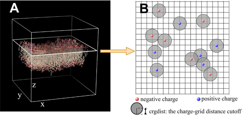
2. MEMPOT
MEMPOT (MEMbrane POTential) uses the potential map to generate the electrostatic
potential profile of membrane while avoiding artificial contributions from grid points being too
close to charged atoms or ions. The structure of the membrane is placed in a grid box defined by
N*N*N periodic grids (users need to make sure that the surface of the membrane is set along the
plane defined by the x and y axes whereas the z axis is parallel to the membrane normal).
MEMPOT is used to calculate the profile of average potential value along z-axis, which is a
macroscopic quantity independent of the position along the x-y plane. For more details, please
refer to:
Roberta P. Dias, Lin Li, Thereza A. Soares and Emil Alexov, Modeling the Electrostatic Potential
of Asymmetric Lipopolysaccharide Membranes: The MEMPOT Algorithm Implemented in DelPhi, Journal
of Computational Chemistry, DOI: 10.1002/jcc.23632Schematic figure of MEMPOT
3. MULTI-DIELECTRIC CODE
Earlier versions of DelPhi handle a scenario where a single molecule is immersed in a
solution. In other words, only a "two-media" world was considered. In the present version, a system
with many different objects having different dielectric constant can be modeled. These objects can
be either sets of atoms obtained from a pdb file or geometric objects.
Note: In order to gain better accuracy for reaction field energy, the location of polarization charges
is normally projected onto the molecular surface. If a molecule is immersed in an object, the
molecular surface would be built inside the object. If two molecules with different dielectric
constants come in contact or overlap, the molecular surface at their interface is not built. (In fact, it
doesn't make sense to do so in that case.) Instead, the polarization charges are not projected
anywhere but are left at their own grid point locations.
Return to new features
4. NON-LINEAR PBE SOLVING ROUTINE
An algorithm has been implemented that can solve the non-linear PBE, as described in
Rocchia et. al. Journal of Physical Chemistry B paper. A good relaxation parameter must be usedYou can also read