WP/20/102 Debt, Investment, and Growth in Developing Countries with Segmented Labor Markets
←
→
Page content transcription
If your browser does not render page correctly, please read the page content below
WP/20/102

Debt, Investment, and Growth in Developing
  Countries with Segmented Labor Markets

    By Edward F. Buffie, Luis-Felipe Zanna, Christopher Adam,
          Lacina Balma, Dawit Tessema, and Kangni Kpodar
© 2020 International Monetary Fund                                                                             WP/20/102

                                                IMF Working Paper
     Institute for Capacity Development, Research Department, and Strategy, Policy, and Review
                                            Department
    Debt, Investment, and Growth in Developing Countries with Segmented Labor Markets†

                  Prepared by Edward F. Buffie, Luis-Felipe Zanna, Christopher Adam,
                           Lacina Balma, Dawit Tessema, and Kangni Kpodar

          Authorized for distribution by Valerie Cerra, Chris Papageorgiou, and Johannes Wiegand

                                                       June 2020

Disclaimer: This document was prepared before COVID-19 became a global pandemic and resulted in
unprecedented economic strains. It, therefore, does not reflect the implications of these developments and
related policy priorities. We direct you to the IMF Covid-19 page that includes staff recommendations
with regard to the COVID-19 global outbreak.

                                                       Abstract
We introduce a new suite of macroeconomic models that extend and complement the Debt, Investment, and
Growth (DIG) model widely used at the IMF since 2012. The new DIG-Labor models feature segmented
labor markets, efficiency wages and open unemployment, and an informal non-agricultural sector. These
features allow for a deeper examination of macroeconomic and fiscal policy programs and their impact on
labor market outcomes, inequality, and poverty. The paper illustrates the model's properties by analyzing
the growth, debt, and distributional consequences of big-push public investment programs with different
mixes of investment in human capital and infrastructure. We show that investment in human capital is much
more effective than investment in infrastructure in promoting long-run economic development when
investments earn their average estimated returns. The decision about how much to invest in human capital
versus infrastructure involves, however, an acute intertemporal trade-off. Because investment in education
affects labor productivity with a long lag, it takes 15+ years before net national income, the private capital
stock, real wages for the poor, and formal sector employment surpass their counterparts in a program that
invests mainly in infrastructure. The ranking of alternative investment programs depends on the
policymakers' social discount rate and on the weight of distributional objectives in the social welfare
function.
JEL Classification Numbers: E62, F34, H54, H63, I25, I31, O43.
Keywords: Public Investment, Growth, Debt, Fiscal Policy, Human Capital, Labor Markets, Welfare.
Authors’ E-Mail Addresses: ebuffie@indiana.edu; fzanna@imf.org; christopher.adam@qeh.ox.ac.uk;
                           l.balma@afdb.org; dtessema@imf.org; kkpodar@imf.org

† We thank Andy Berg, Chris Papageorgiou, Mark Flanagan, S M Ali Abbas, Giovanni Melina, Tom Best, Mariano Moszoro,

and Samuele Rosa for useful comments. All errors remain ours. This joint AfDB-IMF research has been done in collaboration
with the Macroeconomic Policy, Forecasting and Research Department of the African Development Bank (AfDB), and was
generously supported by the AfDB under the KOAFEC Trust Fund, and the IMF under the DFID-IMF Macroeconomic
Research in Low-Income Countries program. The views expressed in this paper are those of the authors and do not necessarily
represent the views or policy of the IMF, DFID, or the AfDB. Working Papers describe research in progress by the authors
and are published to elicit comments and to further debate.
2

                                                          Table of Contents                                                               Page

I. Introduction ..........................................................................................................................4

II. Efficiency Wages, Productivity Gaps, and Segmentation: A Short, Idiosyncratic Survey
    of the Literature....................................................................................................................9

III. The DIG-Labor 1 Model ....................................................................................................21
     A. Technology....................................................................................................................22
         A.1. Production Functions ...........................................................................................22
         A.2. Factor Demands ...................................................................................................22
     B. Preferences ....................................................................................................................23
         B.1. Household Optimization Problems ......................................................................23
     C. Labor Market Features ..................................................................................................26
         C.1. The Effort Function ..............................................................................................26
         C.2. Efficiency Wages, Unemployment, and Underemployment ................................27
         C.3. Sectoral Labor Supply ..........................................................................................27
     D. The Public Sector ..........................................................................................................28
         D.1. Public Investment in Infrastructure ......................................................................28
         D.2. Public Investment in Human Capital ...................................................................29
         D.3. Fiscal Adjustment and the Public Sector Budget Constraint ...............................29
     E. Market-Clearing Conditions and External Debt Accumulation ....................................31

IV. Calibration of the Model and Solution Technique .............................................................32
    A. Linking Some Parameters to Elasticities and Rates of Return......................................32
    B. Base Case Calibration ...................................................................................................34
        ..........................................................................................................................................
V. The Long-Run Trade-offs of Different Types of Public Investment .................................42
    A. Increasing Investments One at a Time ..........................................................................42
    B. The High Cost of Underfunding Maintenance ..............................................................44
    C. Big-Push Investment Programs .....................................................................................46
    D. Pure vs. Mixed Investment Programs ...........................................................................46
    E. Ranking Some of the Contenders ..................................................................................47

VI. The Transition Path ............................................................................................................47
    A. Growth and Structural Change ......................................................................................48
    B. Fiscal Adjustment and Debt Dynamics .........................................................................49
    C. Blended Public Investment Programs ...........................................................................50
    D. Intertemporal Trade-offs: Summary .............................................................................50

VII. Welfare Calculations ........................................................................................................51

VIII. Where to From Here? ......................................................................................................53

References ...............................................................................................................................55
3
Tables
Table 1. The DIG-Labor Suite of Models: Alternative Specifications ....................................67
Table 2. Unemployment Rates in Less-Developed Countries .................................................68
Table 3. Calibration of the Model ............................................................................................69
Table 4. Long-Run Effects of Increasing One Component of Public Investment ...................71
Table 5. The High Cost of Neglecting Maintenance ...............................................................73
Table 6. Long-Run Effects of Big-Push Programs That Increase Public Investment .............74
Table 7. Comparison of Welfare Gains in the Base Case Ru = Rb = 0.30 (ε3 = 5) ...................76
Table 8. Comparison of Welfare Gains when Ru = Rb = 0.20 (ε3 = 5) .....................................77
Table 9. Comparison of Welfare Gains when Ru = Rb = 0.15 (ε3 = 5). ....................................78
Figures
Figure 1. Correcting Sub-Optimal Maintenance Is a Free Lunch ............................................79
Figure 2. Relationship Between Marginal General Equilibrium Returns and the Impact
of the Investment Mix on Long-Run Output ...........................................................80
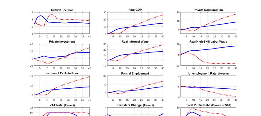
Figure 3. Transition Paths for All-Infrastructure and All-Human Capital (Education)
Investment Programs ...............................................................................................81
Figure 4. Transition Paths for All-Infrastructure and Mixed Investment Programs ................82
Appendices
A. Formal Sector Wage Premium and the Earnings Gap Between the Informal Sector
and Agriculture ............................................................................................................83
B. Wage Curves and Unemployment ...............................................................................91
4

                                       I.    Introduction

   Big-push public investment programs …nanced by external debt remain the policy of choice for
increasing growth and combatting poverty in developing countries (African Development Bank, 2018).
These programs are envisaged to close serious infrastructure gaps, which are pervasive in these coun-
tries, as well as help achieve several sustainable development goals, including those related to health
and education. Moreover, as climate change continues unabated, developing countries will need to
invest in mitigation and adaptation technologies to respond to natural disasters.

   How can policy makers decide whether to implement ambitious public investment programs? And
how can they assess the macroeconomic e¤ects of such programs, including on growth and debt? These
are not simple questions. After all, these decisions and e¤ects may depend on several factors, such
as the needs in speci…c sectors, the prospects for sustainable …nancing (debt-…nanced versus budget
neutral), and the e¢ ciency and return of public investment. But even if policy makers are aware of
these factors, and their role, how can they quantify the macroeconomic e¤ects of public investment
scale-ups?

   To help answer these questions, the Debt, Investment, and Growth (DIG) model and the important
extension for natural resource rich countries, the Debt, Investment, Growth and NAtural Resources
(DIGNAR) model, were developed at the International Monetary Fund (IMF) — see Bu¢ e et al.
(2012), Melina et al. (2016), and Zanna et al. (2019). These models have gained a wide measure
of acceptance in the policy world. Over the past eight years, the DIG and DIGNAR models have
complemented the IMF and World Bank debt sustainability framework (DSF) analysis with over 65
country applications (Gurara et al., 2019). They have provided useful insights in the context of IMF
programs and surveillance work, based on qualitative and quantitative analysis of the macroeconomic
e¤ects of public investment surges.

   The DIG and DIGNAR models have their share of shortcomings, however. Most notably, the
assumption of perfect wage ‡exibility and integrated labor markets is restrictive and increasingly
unappealing. Open unemployment and underemployment are enduring, troublesome facts of life in
many Low-Income Countries (LICs). The models shed light on how public investment programs a¤ect
aggregate labor demand in such countries, but they cannot speak directly to policy makers desire to
reduce inequality and create more good jobs. The omission of rich and more realistic labor markets in
these models is not surprising. To a great extent, the analysis of labor markets in developing countries
has not been central to the progress of development economics in the last two decades (Teal, 2011).
But the need to incorporate richer labor markets in models that can inform policy decisions seems
imperative, as argued by Fields (2011a):
     “I brie‡y highlight four priority areas for future research....The second is the need for
5
empirically grounded theoretical labor market models that can be used in the formulation
of policy. There is some value in developing single-sector models and representative agent
models, but it would be more helpful to have multi-sector models in which labor markets are
segmented, incorporating the key features of labor markets in the country being analyzed.”
In this paper, we present three new models: DIG-Labor 1, DIG-Labor 2, and DIG-Labor 3. Seg-
mented labor markets are front and center in each model. Firms in the formal sector pay e¢ ciency
wages (EWs), while ‡exible wages prevail in agriculture. The third sector, the non-agricultural infor-
mal sector, is populated by wage employees in DIG-Labor 2 and by own-account workers in DIG-Labor
1 and DIG-Labor 3. In DIG-Labor 2, informal …rms pay an EW below the wage in the formal sector.
DIG-Labor 1 and 3 assume that labor earns the same return in the informal sector as in agriculture.
The preferred model depends, of course, on the country under examination. DIG-Labor 1 is appro-
priate for most LICs, DIG-Labor 2 for most Middle-Income Countries (MICs) and Emerging Market
Economies (EMEs), and DIG-Labor 3 for countries that su¤er only from underemployment.
DIG-Labor 1-3 di¤er in the type and severity of the distortions that impair e¢ ciency in the labor
market (Table 1). There is open unemployment in DIG-Labor 1 and 2, but not in DIG-Labor 3.
Furthermore, while involuntary unemployment pervades the entire non-agricultural sector in DIG-
Labor 2, in DIG-Labor 1 it is con…ned to the formal sector. Underemployment is a problem in all
three models: for any given unemployment rate (zero in DIG-Labor 3), aggregate labor productivity
increases when labor moves from the informal to the formal sector or from agriculture to either non-
agricultural sector. In DIG-Labor 1 and 3, labor in smallholder agriculture receives its marginal value
product plus a share of (implicit) land rents. Importantly, however, property rights are insecure or
non-existent; consequently, though labor mobility enforces equal pay in agriculture and the informal
sector, the marginal value product of labor is lower in agriculture.1 The same distortion may operate
in DIG-Labor 2. But even when it does not, the EWs paid in the informal sector exceeds the marginal
value product of labor in agriculture.
The DIG-Labor models contain a number of other new features besides segmented labor markets
and a third sector. They incorporate skilled labor and public investment in human capital; maintenance
investment as well as new investment in infrastructure; and sector-speci…c taxes on wages, pro…ts, and
consumption. These new features allow policy makers to specify the program for public investment and
supporting …scal adjustment in greater detail and to evaluate more accurately its impact on inequality,
1
80 - 95 percent of land is untitled in most of Sub-Saharan Africa (Doss et al., 2015; Chen, 2017). Ejidos in Mexico
and public land in China and Vietnam are other examples of communal land tenure systems where the “use it or lose
it” principle applies. Chen (2017) and Gottlieb and Grobovsek (2019) analyze how such systems distort the allocation
of labor, calibrating their models to Malawi and Ethiopia, respectively. Both …nd large gains from removal of communal
land tenure. See also Wichern et al. (1999) and Thurlow and Wobst (2004) for discussions of how the lack of property
rights for land inhibits rural labor mobility. Otsuka and Place (2001) and Otsuka (2007) emphasize this and other
e¢ ciency losses in Africa caused by the lack of individualized property rights to land.6
growth, unemployment, and underemployment. DIG-Labor 1-3, like DIG, are supported by Dynare
+ MATLAB programs that display the model solutions in graphs and tables. The programs are fully
annotated and very user friendly.
The rest of the paper is organized into …ve sections. Before getting knee-deep in the equations,
we take some space in Section II to survey the empirical evidence bearing on the size of the formal
sector wage premium, the relevance of EWs, and the magnitude of unemployment, underemployment,
and sectoral gaps in labor productivity. A consistent, if variegated, picture emerges from diverse
strands of the literature. Labor markets are highly segmented in most developing countries, but the
textbook model of competitive, ‡ex-wage labor markets applies in some cases and di¤erent types of
segmentation predominate at di¤erent points on the development spectrum. The cliché that one size
does not …t all is correct: development macroeconomics needs to supply policy makers with choice
from a small suite of models.
Sections III and IV develop and calibrate the DIG-Labor 1 model. Following this, we conduct
policy experiments in Sections V-VII. The experiments are fewer in number but wider in scope than
in Bu¢ e et al. (2012) and Zanna et al. (2019). We delineate how the structure of the labor market
and the split between maintenance investment, new infrastructure investment, and human capital
investment in the big push program condition not only the prospects for debt dynamics and growth
but also the impact on inequality, poverty, the supply of good jobs, and social welfare. The optimal
investment program depends on how policy makers evaluate several di¢ cult trade-o¤s and on their
educated guesses for investment returns. Elaborating:
Investment in human capital is much more e¤ ective than investment in infrastructure in pro-
moting long-run economic development when investments earn their average estimated returns.
Investing one percent of GDP in basic education increases aggregate consumption 10:2 percent
and real income of the poor 10:3 percent across steady states. The corresponding numbers are
9:3 percent and 18:1 percent for investment in upper-level education (secondary + tertiary) and
4:3 percent and 5:4 percent for investment in infrastructure. The large disparity in economy-wide
returns and gains for the poor re‡ect in equal parts higher partial equilibrium capital rentals
and stronger pro-growth general equilibrium e¤ects — more crowding-in of private capital and
bigger reductions in unemployment and underemployment — for investment in human capital.2
The decision about how much to invest in human capital versus infrastructure involves an acute
intertemporal trade-o¤ . Investment in education a¤ects labor productivity with a 6- to 8-year
lag. Consequently, it takes 15+ years before net national income, the private capital stock, real
2
The internal rates of return for basic and upper-level education in the base case map into partial equilibrium capital
rentals ten percentage points above the rental for infrastructure.7
wages for the poor, formal sector employment, etc., surpass their counterparts in a program that
invests mainly in infrastructure.
Big-push investment programs that emphasize human capital require more supporting …scal ad-
justment. The delayed impact on growth delays the arrival of endogenous revenue gains in
programs that invest heavily in human capital. Increasing the share of human capital in the
investment program therefore entails more …scal adjustment to avoid explosive debt dynamics
and/or tolerance of a higher debt trajectory for several decades.
Investing in basic education increases growth more but reduces poverty less than investment in
upper-level education. Investment in basic education directly increases the productivity of low-
skill labor. It is not, however, the public investment best suited to combatting poverty. That
honor belongs to investment in upper-level education. Investment in secondary and tertiary
education converts some workers who would otherwise be unskilled and poor into high-skill,
well-paid workers. Moreover, workers who remain low-skill bene…t indirectly. They decrease in
number while the increase in the supply of high-skill labor raises their productivity. Thus, the
demand curve for low-skill labor shifts to the right as the supply curve shifts to the left. The
resulting increase in real wages for workers who remain low-skill combined with the jump in
earnings for the newly skilled produces gains for the ex ante poor far above the gains generated
by investment in infrastructure and basic education.
The share of human capital in the optimal investment program is on the order of 50-100 percent in
the base case.3 The long-run general equilibrium returns on investment in basic and upper-level
education greatly exceed the long-run return on investment in infrastructure in the base case
(see the …rst bullet). This pushes the share of human capital in the optimal investment program
toward 100 percent. On the other hand, diminishing returns, strong gross complementarity of
human capital and infrastructure, and the faster payo¤ to infrastructure all pull in the opposite
direction, toward some type of mixed investment program. The optimal investment share for
human capital depends on (i) policy makers’ willingness, as measured by the social discount
rate, to trade smaller development gains in the short/medium run for larger gains in the long
run and (ii) the weight of distributional objectives in the social welfare function. In the base
case, the optimal investment share is 50 - 75 percent as long as the social discount rate is 0:93
- 0:96 — i.e., no more than three percentage points above the private discount rate (0:93) —
and the weight on the distributional objective is not too extreme. At social discount rates above
0:96, the share for infrastructure drops to zero.
3
We are using the term “optimal” very loosely here. The welfare results presented in Section VII demarcate the zone
containing the optimal share for infrastructure investment, conditional on our educated guess that allocating one-third
of human capital investments to upper-level education is roughly optimal.8
Human capital maintains a sizeable share in the optimal investment program even when internal
rates of return for education are 30-40 percent below their average estimated returns. In line with
the empirical evidence, the base case assumes a partial equilibrium (social) internal rate of return
(IRR) of 12 percent for investment in basic education and 10 percent for investment in upper-
level education. Many development economists reject these IRRs as too high on the grounds
that they are inconsistent with the dismal scores reported for LICs in international achievement
tests. We don’t know whether the sceptics are right or wrong. But even if they are right, a strong
case can be made for allocating a sizeable share to human capital in the optimal investment pro-
gram. Lowering the IRR to 6:7 percent for investment in upper-level education and 7:6 percent
for investment in basic education depresses the long-run partial equilibrium capital rentals for
both investments to 15 percent, …ve percentage points below the capital rental for infrastructure.
Large pro-growth, poverty-reducing general equilibrium externalities substantially compensate
for this handicap. The share of human capital in the optimal investment program is 40 - 65
percent when the social discount rate equals or exceeds 0:96. It drops to 0 - 25 percent at lower
discount rates, but it bounces back up to 25 - 50 percent if education is awarded 20 basis points
as a merit good in calculating the equivalent variation welfare gain.
The …nal section takes up the question of whether the suite of models currently on tap for policy
makers needs to expand. We believe DIG-Labor 1-3 cover a lot of ground, but some countries fall
between the gaps, given the complexities of their labor markets. As such, we foresee further extensions
that include other labor market structures as well as health as a separate component of human capital.
Extending DIG-Labor 1-3 is consistent with the broad agenda of tailoring models to country speci-
…cities and needs. Over the years, the DIG model has been extended to incorporate other dimensions,
such as an energy sector (Issoufou et al., 2014), the cost of operations and maintenance of infrastructure
(Adam and Bevan, 2014), climate resilient infrastructure to address natural disaster shocks (Marto et
al., 2018), and security spending (Aslam et al., 2014), among others. Special mention must be made
of the extension by Atolia et al. (2019), who explore the trade-o¤s between investing in economic in-
frastructure vs. investing in social infrastructure (schools). Our results on the intertemporal trade-o¤s
for real output and …scal adjustment are qualitatively similar to theirs. But their model di¤ers from
our framework mainly in the speci…cation of the labor market and the degree of structural detail —
they consider a representative-agent one-sector model with full employment and a single homogeneous
type of labor. As mentioned before, by incorporating segmented labor markets, EWs, open unem-
ployment, and an informal non-agricultural sector, the DIG-Labor 1-3 allow for a deeper examination
of macroeconomic and …scal policy programs and their impact on labor market outcomes, inequality,
and poverty.
After the literature review in Section II, we focus solely on DIG-Labor 1. Eighty percent of the9
equations in DIG-Labor 1, however, carry over to DIG-Labor 2 and DIG-Labor 3. What di¤ers is the
speci…cation of the labor market. We present the models for DIG-Labor 2 and DIG-Labor 3 in full
and discuss their general architecture in online appendices available at http://pages.iu.edu/~ebu¢ e.
In the case of DIG-Labor 2, we also discuss suitable parameter values for calibration of the model to
MICs and EMEs.
II. E¢ ciency Wages, Productivity Gaps, and Segmentation: A
Short, Idiosyncratic Survey of the Literature
Labor markets in developing countries are complicated and confusing. The empirical literature
relevant to the DIG-Labor models is large and sprawls over several areas. In this section, we survey
the literature, looking for answers to seven questions that determine the correct speci…cation of the
labor market.
Question 1 : How large is the formal sector wage premium?
Short Answer : Very large.
Appendix A contains capsule summaries of 38 empirical estimates of the formal sector wage pre-
mium dating back to 1980. The studies di¤er in the type and quality of data and the extent to
which they control for self selection, observable and unobservable human capital characteristics, and
workplace conditions. Unsurprisingly, the results also di¤er. The size of the reported premium di¤ers
widely not only across countries but also across studies of the same country and even studies of the
same country by the same author. While this is slightly disconcerting, the weight of the evidence
argues that the formal sector wage premium is ubiquitous and large, ranging from 10 - 30 percent at
the low end to 30 - 70 percent in the middle and 70 - 150 percent at the high end.
These numbers re‡ect a certain de…nition of the wage premium and a certain way of reading the
literature. Many studies compute the wage premium from the coe¢ cient on the dummy variable for
formal sector employment, controlling for …rm size and industry category. Typically the wage variable
is the gross base wage; but it is common practice, when the data allow, to compare the wage in the
informal sector to the wage net of taxes and employee social security contributions in the formal sector.
The logic behind this approach to calculating the wage premium is defensible. Controlling for
…rm size and industry category can help control for the impact of workplace conditions on the wage
distribution. Subtracting social security contributions of employees as well as income taxes may be
justi…ed when the connection between mandatory contributions and future bene…ts is tenuous (e.g.,10
as in universal programs) and the objective is to compare net earnings in the formal and informal
sectors.
Our views on the results reported in the literature is that often they are easy to misinterpret and
therefore potentially misleading. For a variety of reasons, EW models predict that large …rms would
pay higher wages than small …rms and that industry would pay more than agriculture.4 Moreover,
micro/small …rms reside mainly in the informal sector and medium/large …rms mainly in the formal
sector. This points to the conclusion that EW e¤ects, which operate most strongly in non-agriculture
and at large …rms, are the source of the wage premium. Accordingly, the formal sector wage premium
should be calculated from the coe¢ cient on the formal sector dummy and the coe¢ cients on …rm size
and industry category dummies, not from the formal sector dummy alone, which captures merely the
e¤ect of formal status per se. In principle, the coe¢ cients on …rm size and industry dummies should
be marked down to re‡ect the in‡uence of any compensating di¤erential paid in the formal sector for
less agreeable workplace conditions. In practice, this is not necessary. As we emphasize in the answer
to Question 2, the evidence suggests that workplace conditions favor the formal sector.
For models like DIG-Labor, there is another problem: with rare exceptions, empirical studies
estimate one wage premium when two are needed. Much of the literature focuses on how after-tax
wages vary by sector in an e¤ort to ascertain whether …rm demand is the operative constraint on
employment in the formal sector. This information is valuable, but it needs to be supplemented with
information from a second measure of the wage premium. Allocative e¢ ciency depends on how the
cost of labor for …rms di¤ers across the formal sector, the informal sector, and agriculture. The input
required for calculation of this wage premium is the pre-tax wage plus all non-wage bene…ts …nanced
by the …rm, irrespective of whether employees value the bene…ts at one cent or one hundred cents
on the dollar. Non-wage bene…ts matter only in the formal sector and vary considerably across the
development landscape: negligible in some countries, they add up to 40 - 90 percent of the base wage
in many others (e.g., Egypt, Mexico, Colombia, Brazil, India, Zimbabwe, South Africa, Panama, and
Bolivia).5
A few examples may help underscore the importance of reading the results in the literature with
a discerning eye. In a widely cited paper, Pratap and Quintin (2006) assert that “once we match
formal sector workers with informal sector workers with similar propensity scores, the formal sector
premium disappears....observably similar workers earn similar wages across sectors in Argentina.”But
the …rm size e¤ect alone generates a formal sector wage premium of 27:1 percent, and factoring in
payroll taxes pushes the cost of labor in the formal sector 49:3 percent above that in the informal
4
The incentive to pay EW is greater for large …rms because management and supervision of the workforce is more
di¢ cult and the costs of labor turnover and idle equipment are higher when technology is more complex and capital
intensive. See Fafchamps and Soderbom (2006) for compelling evidence of EW e¤ects in African manufacturing.
5
See Levy (2008), Ulyssea (2010), Fields (2011b), Joumard and Velez (2013), and Tansel et al. (2015).11
sector. Badaoui et al. (2010) take a similar line, proclaiming that in Ecuador “the formal sector wage
premium is just a …rm size wage di¤erential” when comparing wages net of taxes. As do Tansel and
Kan (2012): “....unobservable …xed e¤ects when combined with controls for individual and employment
characteristics explain the pay di¤erentials between formal and informal employment entirely. The
implication is remarkable....segmentation may not be a stylized fact of the Turkish labor market as
previously thought.”But incorporating the …rm size e¤ect and making the comparison for gross wages
in Ecuador and for gross wages plus all social security contributions in Turkey delivers formal sector
(employer) wage premiums of 47 percent and 72 percent, respectively. We could go on. Other examples
include MacIsaac and Rama (1997), Maloney (1999), Ja¤rey et al. (2006), Botelho and Ponczek (2006),
Baskaya and Hulagu (2011), and Bargain and Kwenda (2014).
Question 2 : Might unobservable heterogeneity in workers’ characteristics and workplace
conditions explain most of the large formal sector premium?
Short Answer : No, subject to the quali…cation that the …ndings of empirical economics are
never fully dispositive.
Three distinct types of evidence rebut this conjecture. First, while many studies do not adequately
control for the possibility that self-selection on unobservable characteristics may determine both an
individual’s sector of employment and their earnings, some do. Studies that exploit panel data to
track the wages of individuals who move between sectors control for unobservable heterogeneity and
sidestep numerous other vexing estimation issues. These studies — the gold standard in the literature
— a¢ rm that the formal sector wage premium is very large.6 To give but one example, Funkhouser
(1997b) …nds that the low-skill wage premium in El Salvador is 61:4 percent for females and 107
percent for males.
Second, the data for both developed and less-developed countries show very high correlations of
inter-industry wage di¤erentials across all occupations, not just occupational groups that work closely
together.7 This robust stylized fact is consistent with EW models that emphasize the connection
between work e¤ort and internal norms for fairness and horizontal equity (e.g., Akerlof, 1982), but
not with the hypothesis that unobserved di¤erences in ability and workplace conditions play a signif-
icant role in determining the formal sector wage premium — it is not credible that time and again
compensating di¤erentials would be the same for widely di¤erent occupational groups in di¤erent
industries.
Third, there is a fair bit of evidence that workplace conditions are generally better in the formal
6
Alvarez (2020) is a notable exception.
7
In Brazil, for example, the correlation coe¢ cient between the wage premiums for managers and security workers is
an astonishing 0:896 (Abuhadba and Romaguera, 1993).12
sector than in the informal sector. Access to phones, electricity, restroom facilities, running water, and
shelter from inclement weather; stability of income; less exposure to myriad environmental hazards;
and lower injury rates all favor the formal sector. Fields (2011a) has this picture in mind when he
avers that “Apart from low earnings levels and lack of social protections, a large number of jobs [in
the informal sector] are downright miserable.”
Assessments based on direct observation will be discounted by some as soft, unreliable data. We
would disagree in this case because observations on access to running water, restroom facilities, etc.,
do not lend themselves to misinterpretation. Moreover, evidence from scattered pieces of hard data
support Fields’assessment: (i) workers in Colombia give the formal sector much the highest scores for
workplace conditions and job characteristics;8 (ii) employees at large …rms in Trinidad and Tobago
engage in less search on the job than employees at small …rms, suggesting greater job satisfaction in
the formal sector (Marcelle and Strobl, 2003); and (iii) inclusion of detailed controls for the workplace
environment have either no e¤ect or a positive e¤ect on the formal sector wage premium in Zimbabwe
(Velenchik, 1997), Peru (Scha¤ner, 1998), and Brazil (Arbache, 2001).9 Echoing Fields’view, Arbache
observes that the positive results for Brazil “seem to be in accordance with LDC’s labor market charac-
teristics....poverty [pushes] poor people to take unpleasant and riskier jobs without being appropriately
compensated.”
We segue to the next question with a caveat. The case built here against compensating di¤erentials
pertains only to the comparison of wage employment in the formal sector with earnings in agriculture
and wage employment in the informal sector; the comparison vis à vis self-employment in the informal
sector is less clear-cut.
Question 3 : How heterogeneous is the informal sector? More speci…cally, does the formal
sector wage premium vary signi…cantly vis-à-vis di¤erent segments of the informal sector?
Short Answer : It depends on the country in question.
The informal sector is heterogeneous. It comprises, at a minimum, two distinct segments: salaried
workers and the self-employed (owners of micro enterprises, independent professionals, and own-
account workers). The relative importance of the two segments varies considerably from one developing
country to the next. Self-employment accounts for 70 - 90 percent of informal employment in most
LICs. In MICs and EMEs the two segments are of equal size or wage employment predominates.
8
The …ndings in the special module on Quality of Employment in Colombia’s 1994 National Household Survey are
discussed in Goldberg and Pavcnik (2003).
9
The United States can be added to the list of countries where the hedonic wage premium is larger than the non-
hedonic premium (Krueger and Summers, 1987 and 1988). This will come as no surprise to anyone who has read Barbara
Ehrenreich’s Nickle and Dimed (2001).13
Typically, salaried workers in the informal sector strongly prefer employment in the formal sector,
where pay is much higher and workplace conditions much better. For the self-employed, the results
are more mixed. According to labor force surveys for Latin America and the Caribbean, the majority
of the self-employed do not seek jobs in the formal sector; they work voluntarily in the informal sector
in order to maximize earnings and/or enjoy greater independence (Maloney, 1999, 2002, 2004; Bosch
and Maloney, 2007; Perry et al., 2007). This two-tiered structure also seems to describe the informal
labor market in Côte d’Ivoire (Gunther and Launov, 2012).
But the separation between the two tiers is far from clean. Thirty percent of the self-employed in
the aforementioned surveys for Latin American and Caribbean prefer employment in the formal sec-
tor. In Colombia and Turkey, the self-employed are no better o¤ than wage employees in the informal
sector, and in Ethiopia, Malawi, Tanzania, Uganda, South Africa, and Ghana they earn considerably
less (Perry et al., 2007; Ben Salem and Bensidoun, 2012; McCullough, 2017; Heintz and Slonimcyzek,
2007; Heintz and Posel, 2008). Although hard data is lacking elsewhere, the consensus among informed
observers is that, outside of four or …ve countries in Latin America, work in the informal sector is a
desperate strategy-of-last-resort for both the self-employed and wage employees:
“The enterprises of the poor often seem more a way to buy a job when a more conventional
employment opportunity is not available than a re‡ection of a particular entrepreneurial
urge. Many of the businesses are run because someone in the family has (or is believed to
have) some time on hand and every little bit helps....the many businesses of the poor are
less a testimony to their entrepreneurial spirit than a symptom of the dramatic failure of
the economies in which they live to provide them with something better.” (Banerjee and
Du‡o, 2011)
“Many informal entrepreneurs would gladly close their businesses to work as employees in
the formal sector if o¤ered the choice.” (La Porta and Shleifer, 2014)
“Typically, the better jobs are in wage employment, not self-employment....The problem
the poor face is that not enough regular wage employment is available for all who would
like jobs and are capable of performing them.” (Fields, 2011a)
Question 4 : How strong is the evidence for EWs in the formal sector?
Short Answer : Very strong.
Over the past 20 years, empirical studies have amassed abundant, compelling evidence that EWs
operate throughout the formal sector in less-developed countries (LDCs). Estimates of the impact of
unemployment on real wages con…rm the existence of wage curves in Argentina, Turkey, Colombia,
Uruguay, Chile, South Africa, Côte d’Ivoire, Mexico, China, South Korea, and a host of other LDCs14
(Blanch‡ower and Oswald, 2005). There is also powerful, if indirect, evidence supportive of EWs in
the stylized facts documented in microeconomic studies of developing country labor markets. Across
the development spectrum, wage and employment data exhibit the same patterns: (i) …rm-size wage
premiums that start at very small establishment size (5+ employees) and are much larger than in
developed countries; (ii) persistent, remarkably stable inter-industry wage di¤erentials; (iii) high cor-
relation of industry wage premiums across occupations; (iv) large wage premia for formal vs. informal
sector employment and for informal non-agricultural employment vs. agricultural employment; (v)
large cyclical ‡ows into and out of unemployment in both the formal sector and the informal sector;
(vi) virtually identical lists for low- and high-paying industries; (vii) large, stable wage di¤erentials
between …rms in the same industry; (viii) payment of higher wage premiums in capital-intensive in-
dustries; and (ix) lower quit rates and longer job tenure in the formal sector. At present, only EW
models can explain all of these stylized facts. Competing theories cannot be ruled out altogether —
the sheer number and diversity of LDCs precludes that — but none come close the explanatory power
of EW.10
Question 5 : Are there EWs in the informal sector?
Short Answer : Yes, but only in the wage-employment sub-sector.
We need to elaborate on some of the empirical evidence cited in support of EW in the answer to
Question 4:
Appendix B collects estimates of wage curves that relate the level of the real wage to the un-
employment rate in LDCs. Clearly, wage curves are not con…ned to the formal sector; they
also operate in the informal sector. This does not mean that wages are equally rigid in the two
sectors. The common perception that wages are more ‡exible in the informal sector is correct.
Most studies …nd that wages in the informal sector are more responsive to the unemployment
rate than wages in the formal sector. But a large gap separates more responsive from highly
responsive. The informal sector does not approximate a frictionless bu¤er sector with ‡exible,
market-clearing wages.
The …rm size e¤ect kicks in very quickly, starting at micro enterprises with 2-5 employees (Ve-
lenchik, 1997; Scha¤ner, 1998; Badaoui et al., 2010).
If wages are rigid in the informal sector, the data should show large movements into and out of
unemployment during booms and recessions. This is precisely what Bosch and Maloney (2007)
10
Mixed models are relevant in some countries. EW e¤ects can explain the many puzzling stylized facts associated
with minimum wage increases in less-developed countries. We would also argue that optimizing union models should
incorporate EW e¤ects.15
…nd in their study of labor market dynamics in Mexico, Argentina, and Brazil.11 Salaried jobs
in the informal sector showed high rates of separation toward unemployment and inactivity (i.e.,
dropping out of the labor force). In fact, in all three countries transitions out of informal sector
employment contributed much more to unemployment than transitions out of formal sector
employment. In Mexico, for example, transitions into unemployment from salaried informal
employment were three times greater than transitions from formal employment; equally striking,
none of the workers laid o¤ in the formal sector found jobs in the informal sector — entry from
the formal into the informal sector declined during downturns.
For at least one important country, there is strong, direct evidence of job rationing in the informal
sector. In labor force surveys in South Africa, 80 percent of the unemployed reported that they
could not …nd any work; only three percent cited an inability to …nd “suitable work” as the
reason for being unemployed (Heinz and Posel, 2008). Several other studies corroborate the
survey …ndings. Nattras and Walker (2005) and Burger and Schotte (2017) estimate that the
reservation wage of the unemployed is far below their predicted earnings and link their results to
data showing a shortage of job o¤ers is the principal cause of unemployment; job refusals are rare.
Kingdon and Knight (2004) present data a¢ rming that the unemployed are substantially worse
o¤ than the employed in the informal sector in income, consumption, and various indicators of
non-economic well-being.
Labor force participation rates are implausibly low in much of Sub-Saharan Africa (Falco et al.,
2011; Teal, 2014). The most plausible explanation is that discouraged workers, who cannot …nd
a job even in the informal sector, are misclassi…ed as “out of the labor force.”
Our brief includes one more bullet point. The puzzling stylized facts associated with minimum
wages in LDCs are highly informative about the nature of wage determination in the informal sector:
For a long time, conventional wisdom subscribed to a simple, intuitively appealing account of the
repercussions of raising the minimum wage, to wit: employment decreases in the formal sector;
some of the laid-o¤ workers seek jobs in the informal sector; ergo employment increases and the
real wage falls in the informal sector. But then the facts showed up and ruined a good story.
The narrative goes badly wrong when it shifts to the impact on the informal sector. Sometimes
employment increases in the informal sector; normally, however, it decreases more than employ-
ment in the formal sector (Betcherman, 2014). The real wage in the informal sector does not
decline; re‡ecting the ubiquitous “lighthouse e¤ect,”it almost always increases (Gindling, 2014).
These results are di¢ cult — maybe impossible — to reconcile with a competitive, ‡ex-wage view
11
Berg and Contreras (2004) supply evidence for Chile. Neri (2002) and Ulyssea (2010) provide additional evidence
for Brazil.16
of the labor market, but they make perfect sense if …rms in the informal sector pay EW and the
minimum wage shifts the norm for fairness among workers (Adam and Bu¢ e, 2020).
At the risk of belaboring the obvious, we note that self-employed workers do not pay themselves an
EW. In the self-employment segment of the informal labor market, the “wage”is an implicit payment
for labor services and perfectly ‡exible. The need for multiple DIG-Labor models stems from this
and the tremendous variation in the weight of the self-employed in informal sector employment. DIG-
Labor 1 and DIG-Labor 3 posit ‡exible wages in the informal sector. One or the other is appropriate
for countries where informal employment is largely synonymous with self-employment. For countries
where wage employment predominates in the informal sector, we recommend DIG-Labor 2, although
users who believe wages are ‡exible across the informal sector will choose DIG-Labor 1 or DIG-Labor
3.
Question 6 : Is the marginal value product of labor lower in agriculture than in the infor-
mal sector?
Short Answer : Probably.
Empirical studies of structural transformation and the economic returns to migration from agricul-
ture to non-agricultural work speak to this question. The literature on both suggests that reallocation
of labor from agriculture to other sectors — including the informal sector — generates large increases
in aggregate labor productivity. The reason for hedging with “suggests”in the preceding sentence and
with “probably” in the Short Answer is that doubts persist about the reliability of the data and the
correct interpretation of the results.
The literature on structural transformation decomposes increases in aggregate labor productivity
into within- and between-sector e¤ects. For illustrative purposes, divide the economy into agriculture
and non-agriculture (distinguished by subscripts a and n). Let Li and Yi denote employment and
value added in sector i. Aggregate labor productivity is then
Y Yn + Ya
= ; (1)
L L
which can be expressed as
Y Yn Ya
= `n + `a ; (2)
L Ln La
where L = La + Ln is total labor supply and `i = Li =L is the share of employment in sector i.
Misallocation in the labor market depends on the gap in sectoral marginal value products of labor
(M V P Li ). From (1),
d(Y =L) M V P Ln M V P La
= d`n + Within-Sector E¤ect. (3)
Y =L Y =L
| {z }
True Between-Sector E¤ect17
where the Within-Sector E¤ect is calculated as a residual.
The structural transformation literature takes a di¤erent approach, focusing instead on the gap in
sectoral labor productivity. Simple manipulation of (2) yields
d(Y =L) Yn =Ln Ya =La `n d(Yn =Ln ) + `a d(Ya =La )
= d`n + : (4)
Y =L Y =L Y =L
| {z } | {z }
Between-Sector E¤ect Within-Sector E¤ect
To connect (4) to the theoretically correct decomposition in (3), assume labor is paid its marginal
value product (M V P ) so that
M V P Li M V P Ln n
= i =) = AP G; (5)
Yi =Li M V P La a
where i wi Li =Yi is the cost share of labor in value added and AP G (Yn =Ln )=(Ya =La ) is the
agricultural productivity gap.
Clearly, the Between-Sector E¤ect in (4) is not an exact measure of the contribution of structural
transformation to growth in aggregate labor productivity. In practice, however, it is an acceptable
approximation. The data place n around 0:5 and a between 0:45 and 0:60 (see Section IV). The
measurement error associated with the adjustment factor n= a deviating from unity is not trivial,
but the bias could go in either direction and is small relative to most estimates of AP G. In the metic-
ulous, authoritative study conducted by Gollin et al. (2014), which controls for home production in
agriculture, for di¤erences in the cost of living and urban vs. rural amenities, and for sector di¤erences
in hours worked and in human capital acquired from experience and schooling, the mean AP G for the
poorest quartile of countries is three. Caselli (2005) and Restuccia et al. (2008) also present evidence
of very large AP Gs. Until recently, therefore, there was general agreement that labor productivity in
agriculture is much lower than in non-agriculture and hence that the potential gains from structural
transformation are large, especially in LICs. Back in 2014, in their introduction to a special issue
of World Development on Understanding Structural Transformation in Africa, McMillan and Heady
(2014) could follow the observation that
“The question underlying all this literature is why quasi-subsistence agriculture is so perva-
sive in poor countries, particularly since rural areas seem to be very poor and unproductive
relative to urban areas.”
with the strong, con…dent assertion that
“There is thus a potential for enormous economic gain in African countries from reallocating
activity from low to high productivity sectors. The next set of papers in this special issue
present evidence of signi…cant untapped opportunities for structural change in Africa.”18
That was then. Today the case for large gains from structural transformation is under a cloud of
indeterminate size. Two recent papers challenge the view that the AP G is large on the grounds that
the datasets in Gollin et al. (2014) and a host of other studies rely on labor force surveys that greatly
overstate hours worked in agriculture.
Arthi et al. (2018) test for recall bias in the Mara region of Tanzania by comparing labor input
reported in weekly visits (presumed accurate) with labor input reported after the harvest (the practice
in most agricultural surveys). The disparity in the answers is disturbing. Households surveyed after
the harvest reported hours worked per person per plot 3 - 3:7 times greater than hours reported by
households surveyed weekly. On the basis of this …nding, the authors conclude that previous studies
greatly exaggerate the AP G.
But households surveyed at the end of the agricultural season also underreport the number of
family members engaged in farming by 33 percent and the number of plots cultivated by 47 percent.
After adjusting for these o¤setting errors, overreporting of labor hours decreases to 8:1 percent. The
authors counter that the overlooked plots are likely to be marginal plots and the overlooked family
members working in farming more likely to be children. This is probably true. But we do not know
for sure. And even if the conjectures were known to be true, we do not know how much weight they
carry in the calculation of total labor input. Long-period recall data understate labor productivity,
but the magnitude of the bias is unknown.
McCullough (2017) provides further evidence that standard labor force surveys substantially over-
state hours worked in agriculture. Armed with new rich micro-level household surveys, she decomposes
the gap in output per worker (GAP ) in Ethiopia, Malawi, Tanzania, and Uganda into the product of
the productivity gap (P GAP ) and the employment gap (EGAP ):
Yn =Ln Yn =Hn Hn =Ln
= =) GAP = P GAP EGAP; (6)
Ya =La Ya =Ha Ha =La
where H is hours worked, P GAP (Yn =Hn )=(Ya =Ha ), and EGAP (Hn =Ln )=(Ha =La ).12
The decomposition in (6) reveals tremendous underemployment in agriculture. EGAP ranges
from 2:1 in Uganda to 3:3 in Malawi and explains the majority of GAP . McCullough concludes that
the results “call into question the productivity gains that laborers can achieve through structural
transformation.”
But again, the headline exaggerates. The average productivity gap in the four countries is 1:58.
This is barely half the value for Sub-Saharan Africa in Gollin et al. (2014), but still large in absolute
12
We have changed notation here. In equations (1) - (5), La and Ln refer to employment adjusted for di¤erences in
hours worked in sectors a and n. In equation (6), they refer to the number of employed workers.19
terms. Moreover, Ethiopia is a distinct outlier in both Gollin et al.’s and McCullough’s datasets. The
average productivity gap in Malawi, Uganda, and Tanzania is 1:82.
We have discussed this part of the literature in detail because the number for the AP G has
important implications for the size of the productivity gap between the informal sector and agriculture.
None of the studies cited earlier compute separate AP Gs for the formal and informal sectors. But
the aggregate AP G together with estimates of the formal sector wage premium can be used to tease
out guesstimates of the AP G and M V P L gap for the informal sector component of non-agriculture.
Return to (1) and replace Yn and Ln with Yf + Yj and Lf + Lj , where subscripts f and j refer to the
formal and informal sectors. By de…nition,
(Yf + Yj )=(Lf + Lj ) Yf =Lf Yj =Lj Lf Yj =Lj Lj
AP G =) AP G = + : (7)
Ya =La Yj =Lj Ya =La Lf + Lj Ya =La Lf + Lj
Let `j Lj =(Lj + Lf ), P GAPf j (Yf =Lf )=(Yj =Lj ), and P GAPja (Yj =Lj )=(Ya =La ) denote
respectively the share of the informal sector in non-agricultural employment, the productivity gap
between the formal and informal sector, and the productivity gap between the informal sector and
agriculture. With this notation,
AP G M V P Lj j AP G
P GAPja = =) = : (8)
`j + (1 `j )P GAPf j M V P La a `j + (1 `j )P GAPf j
Consider a LIC where j = 0:8, P GAPf j = 2, and j= a = 0:8 1. For AP G = 3, the mean value
for the poorest quartile of countries in Gollin et al. (2014), equation (8) returns M V P Lj =M V P La =
2 2:5. This is much too large. In line with the critiques in Arthi et al. (2018) and McCullough (2017),
an AP G of three overstates the agricultural productivity gap. An AP G of two, on the other hand,
works quite well. The range for the M V P L gap, 1:33 - 1:67, is consistent with the estimated earnings
gaps of 46 percent, 39 - 46 percent, and 30 percent between informal wage employment and agricultural
self-employment in Ghana, South Africa, and Turkey (Heintz and Slonimczyk, 2007; Heintz and Posel,
2008; Baskaya and Hulagu, 2011); with the 41 percent consumption gain for individuals who moved
from agricultural to non-agricultural work in Beegle et al.’s (2011) tracking study of migration in
Tanzania; and with the sizeable fraction of increased labor productivity in Vietnam and Tanzania
attributable to reallocation of labor from agriculture to informal employment (McCaig and Pavnik,
2013; Diao et al., 2018).
The Catch: As usual, there is a catch. EW can explain the productivity gap between the formal sector
and agriculture. But what explains the M V P L gap between the informal sector and agriculture? If
the gap is truly large, then why isn’t there more rural-urban migration (De Brauw et al., 2014;
Christiaensen and Todo, 2014)? Why doesn’t arbitrage eliminate most or all of the MVPL gap?You can also read