3DVAR in the OPATM-BFM biogeochemical forecast system - Gianpiero Cossarini, Cosimo Solidoro, Anna Teruzzi Giorgio Bolzon

3DVAR in the OPATM-BFM
biogeochemical forecast system

         Gianpiero Cossarini, Cosimo Solidoro,

             Anna Teruzzi

             Giorgio Bolzon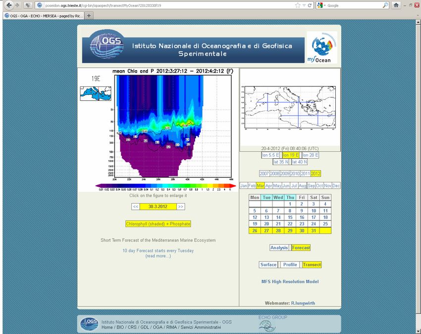

3DVAR in the OPATM-BFM biogeochemical forecast system

3DVAR adapted from the physical assimilation scheme of the INGV
Mediterranean Forecast System (Dobricic and Pinardi, 2008)
3D-VAR scheme iteratively finds the minimum of the following cost function

J = (x − x b ) B (x − x b ) + (H (x) − y ) R −1 (H (x) − y )
   1          T −1           1            T

   2                         2
Equation is linearized around the background state (Lorenc, 1997)
 Introducing:
δx = x − x b        increment
 d = [y − H (x b )] misfit
 H linearization of observation operator at xb

 J = δx B δx + (Hδx − d ) R −1 (Hδx − d )
    1 T −1    1          T

    2         2
B can be written in the form VVT avoiding B inversion and in order to
precondition the minimization, J is minimized using a new control
variable v defined as:

  v = V +δx     V+ is the rectangular pseudoinverse (generalized inverse) of V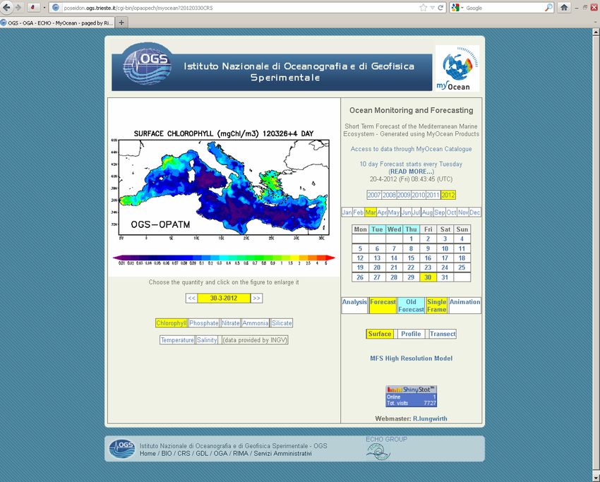

Therefore the cost function has the form of

         v v + (HVv − d ) R −1 (HVv − d )
       1 T    1
  J=
                         T

       2      2

  The minimization using the gradient method

   J ' = v − V T H T R −1 (d − HVv )   Æ J’=0 … compute first guess of v

  J ' ' = I − V T H T R −1HV           Æ Interactive computation of v
                                                v i +1 = v i + J ' '−1 J '

The solution of J(v) needs the adjont of operators V and H (each subroutine
containg the transpose of V and H is hand-coded)

Solution is then transformed from the control space to the physical space:
    δx = Vv
  V can be decomposed into a series of operators:

    V = Vb Vh Vv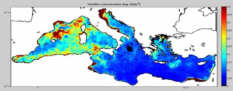

x vector of BFM model state variables
x=[P1i, P1c, P1p, P1n, P1s, P2i, … P3i, … P4i, …]

y observation
5 days centered mean map of surface chlorophyll (MODIS-aqua)
Daily maps of 1/16° resolution with a regional algorithm (L4, Volpe et al.,
2008) by CNR-GOS-ISAC (Rome, Italy)
Delay Time products available at the MyOcean Web Portal after 4 days

R is defined in two ways:
1. 30% of the observation, as generally
indicated for the satellite chlorophyll
concentration data, limited by the model       30%satellite map
error (in order to avoid inefficient
assimilation)
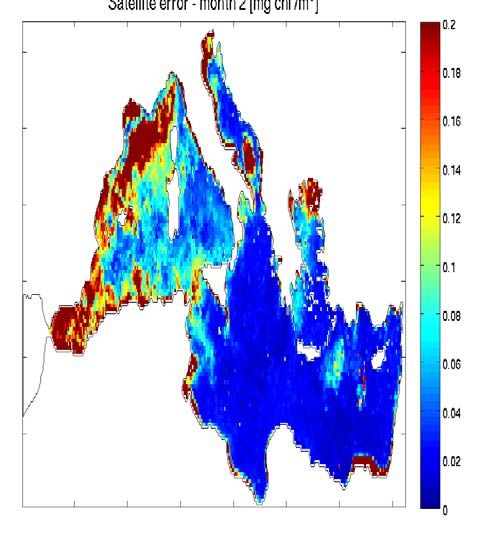
2. Monthly values of satellite observations
variance calculated using 2007–2010 data

Æ Combination of the two terms (constant
+ variable part)

          satellite map)
                                              February st.dev

v Å solution in control space
2D map of EOF coefficients

δx = Vv = VbVhVvv
V operators are applied sequentially (subroutine whose argument is the
previous result)

Vv(v) Æ 3D field of CHLA
through application of
EOF composition

Vh(Vv(v) ) Æ Horizontal
smoothing

x+δx=Vb(Vh(Vv(v)))Æ biological propagation on 4 phytoplankton groups

 P1c,n,p,s,i
                                   P2c,n,p,i

P3c,n,p,i                         P4c,n,p,i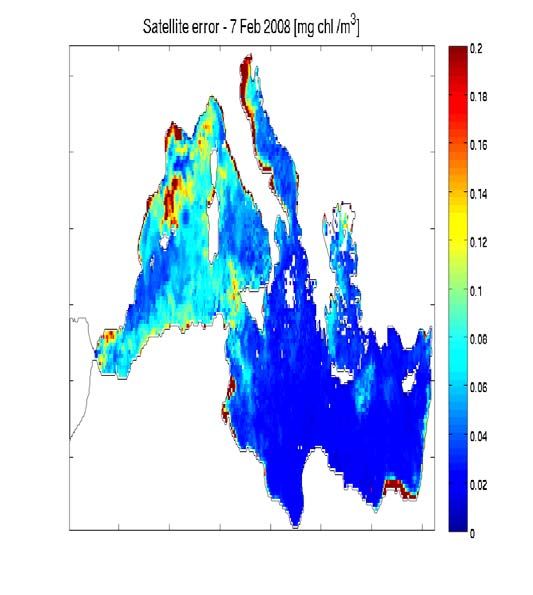

Decomposition of V=VbVhVv

Vv vertical covariance described by EOF = SD1/2 (eigenvectors and diagonal
of eigenvalues matrix)
9 regions Empirical Orthogonal Functions (EOF) of the profiles anomalies
based on multi-annual simulations (1995 – 2004)
Æ one set of EOF for each month
                                                    Feb

   Feb                    Jul                       Feb

  Æ one set of EOF for each grid point (variance modulates the EOFs)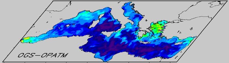

Decomposition of V

Vh propagates the innovation horizontally
  Gaussian smoothing with horizontal correlation radius of 10-100 km
   (testing distances)

                                No data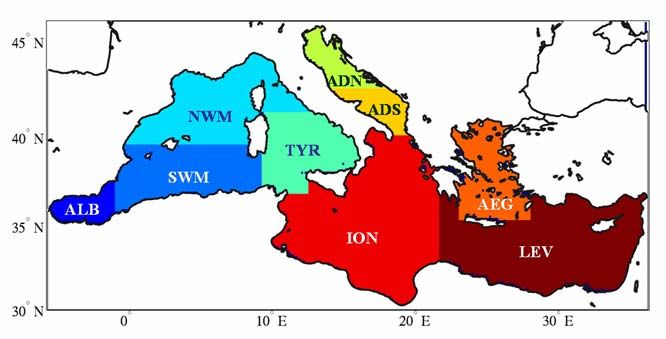

Decomposition of V

Vb innovation on other biogeochemical variables
Phytoplankton groups ratio and elements internal quota preserved
                                  δx'
 x = x 0 + δx'   corrfact = 1 +
                                  x0
CorrFactor is applied to all phytos and phytos components
 P1inew = P1iold ⋅ Corrfactor
 P 2inew = P 2iold ⋅ Corrfactor
         ...........
 P1cnew = P1cold ⋅ Corrfactor
         ...........
 P1nnew = P1nold ⋅ Corrfactor

Vb includes checks:
IF CorrFactor>103 THEN CorrFactor = 1
IF P1n/P1i >150 and P1p/P1i >10 ( maximun nutrient/chlorphyll ration) THEN
CorrFactor = 1
[sinking of dead phytoplankton just below the photic zone (chlorophyll
degradation faster than nutrient release)]

3DVAR in the operational chain of MyOcean biogeochemical
forecast system
Two weekly run executions at CINECA (HPC, Italy)
Friday run
   7 days of hindcast (forced by Med-MFC-currents analysis provide by INGV)
   10 days of forecast (forced by Med-MFC-currents forecast by INGV)
Tuesday run
    7 days of analysis (forced by Med-MFC-currents analysis, ICs via DA)
    10 days of forecast (forced by Med-MFC-currents forecast)

                                  Run execution

               M T W T F S S M T W T F S S M T W T F S
           Restart using
        Friday hyndcast                 Run execution

                       T F S S M T W T F S S M T W T F S S M T

                                   3DVAR using Tuesday forecast and surface
                                   chlorophyll OC TAC centered on Tuesday

                              M T W T F S S M T W T F S S M T W T F S
                                                  Run execution

Operational implementation in the MyOcean Forecast System

    Four steps:
    1. Pre-processing
    2. 3DVar routine
    3. Post-processing and creation of a new restart files and
       ancillaries information
    4. run of a 7 + 10 days forecast

1. Pre-processing

-    Download of daily DT maps of satellite chla from ftp site CNR-ISAC
-    mean of 5 days centered on Tuesday (-> log transformation)
-    bilinear interpolation on 1/8° (at least 2 available data on diagonals)
-    masking points with depth lower than 200 m (new algorithm for OC with
     case 2 waters implemented by CNR-ISAC as new product of MyOcean2)

Computation of R (observation model error covariance matrix)

Computation of d (misfit) , H is a matrix of 0s and sparse 1s )
    d = [y − Hx b ]   d = chlsat − (chlP1 + chlP 2 + chlP 3 + chlP 4 )

2. 3DVAR routine
Code developed by Dobricic (see Dobricic and Pinardi, 2008) for physical
assimilation and adapted for biological data assimilation by OGS

- Computation of cost function and its derivates

- Interactive cycle for computation of v (gradient method)

-computation of   δx = Vv    as subsequent application of the operators

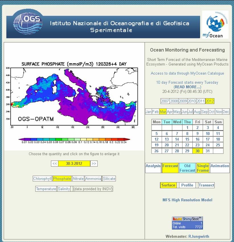
3. Post-procesing and creation of new IC
- Saving information (missfit, assimilated field, obs err covariance
matrix)
- Preparation of IC for next run:
  read of results of BFM variables from previous run and substitution
  of phyto variables (P1c, P1n, P1pi, P1s, P4i for P1,P2,P3 and P4)

4. run of a 7 + 10 days forecast and visualization
- Download of physical forcing from INGV site (7 days analysis and 10
days forecast)
- Setting boundary conditions (Nutrients at rivers and run-off (monthly
for major rivers, constant for run-off)), and open boundary at Gibraltar
(monthly), atmospheric depositions(constant), light estimation factor
(2D monthly maps from satellite)
-Simulation run and data storage (4 hours on CINECA IBM machine)
- Upload of results to the Catalogue of MyOcean site
-Visualization of results into OGS visualization site at
http://poseidon.ogs.trieste.it/cgi-bin/opaopech/myocean/

Visualization of results on OGS website

Visualization of results on OGS website

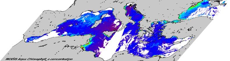
Example of DA results
• The DA postpones the start of the bloom in NWM, then
  model correctly reproduces the bloom in the next 5-
  day-period forecast
• New forecasts show a better consistency with short
  term evolution of satellite observations (timing and
  location of local blooms)

        Forecast                                    Forecast
           2 Feb                                       7 Feb

                          Assimilation
                                2 Feb

        Satellite                                   Satellite
          2 Feb                                       7 Feb