Post-traitement statistique des prévisions d'ensemble à Météo-France - Meteo France
←
→
Page content transcription
If your browser does not render page correctly, please read the page content below

Post-traitement statistique des prévisions d’ensemble à Météo-France

                                             Maxime Taillardat

                                              maxime.taillardat@meteo.fr

                                             12 mars 2019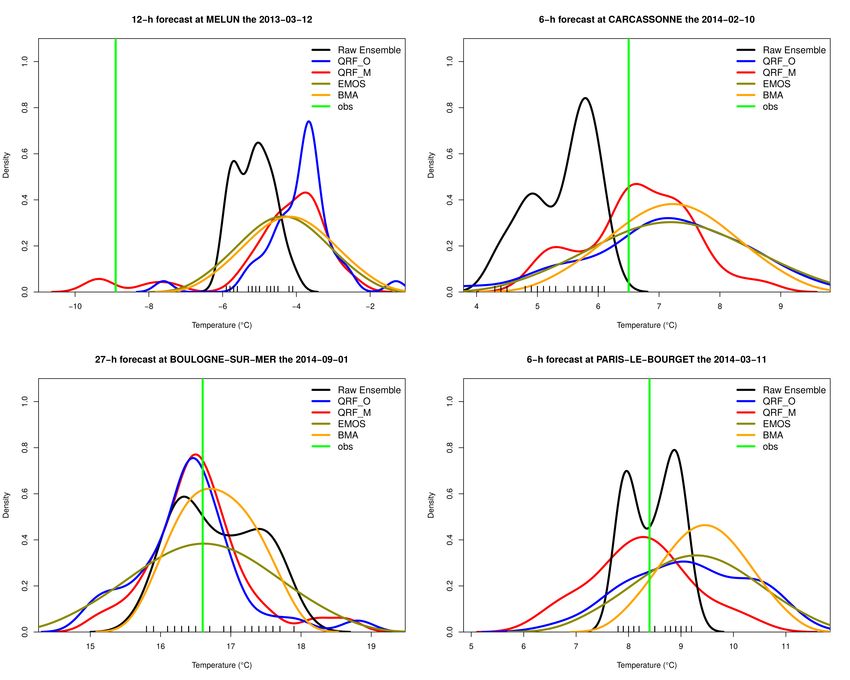
Motivation of post-processing ensemble forecasts

                                                    Run: 2012−10−26 Lead time: 12 h
                                                  Rank of the observed temperature: 18

      Météo-France’s                                                                          forecast
    35-members global                                                                         observed

     ensemble system                        −10   0           10           20            30

     (PEARP), 10 km                                      Temperature (°C)

  resolution over France.

     Observations and
      forecasts of 2-m
   temperature (T2m) at
   Lyon-Bron for the run
   of 1800UTC (different
         lead times)

Maxime Taillardat                  1/16
Motivation of post-processing ensemble forecasts

      Météo-France’s
    35-members global
     ensemble system
     (PEARP), 10 km
  resolution over France.

     Observations and
      forecasts of 2-m
   temperature (T2m) at
   Lyon-Bron for the run
   of 1800UTC (different          ◮   Need of a simultaneous correction of bias and
         lead times)                  dispersion
                                  ◮   Whatever the quality of the raw ensemble,
                                      post-processing improves forecast attributes
                                      (Hemri, 2014)
Maxime Taillardat                  1/16
The state of the art

          ◮   Existing methods: Analogs, Perfect Prog., Rank-based matching,
              CDF-matching, Member dressing, Bayesian Model Averaging, SAMOS...
          ◮   A review of techniques: Gneiting, 2014

      The most (famous // widely-used // efficient) post-processing method :
          ◮   Ensemble model output statistics (EMOS) (Gneiting, 2005) also
              called Non-homogeneous Regression (NR)
                    ◮   fitting parameters linearly on predictors on some training period:
                                                                           X
                                                                           N
                                   f (y |x1 , . . . , xN ) = N (µ = a0 +         ai xi , σ2 = b + cs2 )
                                                                           i=1

                        y response variable, x1 , . . . , xN ensemble member values or any other
                        predictor, s2 ensemble variance

Maxime Taillardat                              2/16
Benefits of non-parametric post-processing

      No assumptions on the weather variable you deal with
         ◮   Raw ensemble (not                 EMOS
             post-processed) :

      Non-parametric

Maxime Taillardat                  3/16
Benefits of non-parametric post-processing

      No assumptions on the weather variable you deal with
         ◮   Raw ensemble (not                 EMOS
             post-processed) :
                                                 ◮   EMOS post-processing :

      Non-parametric

Maxime Taillardat                  3/16
Benefits of non-parametric post-processing

      No assumptions on the weather variable you deal with
         ◮    Raw ensemble (not                    EMOS
              post-processed) :
                                                    ◮   EMOS post-processing :

      Non-parametric
          ◮   Post-processing possible results :

Maxime Taillardat                    3/16
Best-of post-processing possible outputs
(initialization: 18 UTC)
Maxime Taillardat 4/16From binary regression trees to QRF
◮ Example: CART algorithm (Breiman, 1984)
Taillardat, Maxime, Olivier Mestre, Michaël Zamo, and Philippe Naveau.
"Calibrated ensemble forecasts using quantile regression forests and
ensemble model output statistics." Monthly Weather Review 144, no. 6
(2016): 2375-2393.
Maxime Taillardat 5/16How to verify/evaluate ensemble forecasts ?
◮ Differ from deterministic forecasts
◮ A "point" (eg. for one day) verification is a nonsense
◮ It has to be statistical
Several attributes sought
◮ Reliability
◮ Accordance between forecasted probabilities and observed frequencies of
an event and/or exchangeability between observations and ensemble
members
◮ Resolution/Discrimination
◮ Ability to differ from a climatological forecast
◮ Sharpness
◮ Getting the least dispersed forecast
"the paradigm of maximizing the sharpness of the predictive distributions
subject to calibration"(Gneiting et al. 2006)
Maxime Taillardat 6/16How to verify/evaluate ensemble forecasts ?
◮ Differ from deterministic forecasts
◮ A "point" (eg. for one day) verification is a nonsense
◮ It has to be statistical
Several attributes sought
◮ Reliability
◮ Accordance between forecasted probabilities and observed frequencies of
an event and/or exchangeability between observations and ensemble
members
◮ Resolution/Discrimination
◮ Ability to differ from a climatological forecast
◮ Sharpness
◮ Getting the least dispersed forecast
"maximizing the value of the predictive distributions subject to good overall
performance"
Maxime Taillardat 6/16"Here comes the rain again..."
Production constraints
◮ Relatively shallow datasets ( 1 up to 3 years)
◮ Costly reforecasts
Possible alternatives
◮ Data-shifting: Work with anomalies (obs −→ obs − ensemble mean)
◮ Data-pooling: Regionalization/Neighborhood
◮ Data-boosting: Work with several observations/distribution
Maxime Taillardat 7/16"Here comes the rain again..."
Example: post-processing RR6 (6-h rainfall)
◮ This variable is (by far !) the most difficult to calibrate whatever the
method, a really hard nut to crack for statisticians
◮ A lot of zeros, a lot of "extremes"
What we have tested
For EMOS:
◮ Try different distributions "tailored" for extremes (Gamma, GEV...)
◮ Try different sets of predictors
For QRF:
◮ Improve QRF for "quantiles": Gradient Forests (GF) (Athey et al., 2017)
◮ Extrapolation in distributions tails: semi-parametric approach
Maxime Taillardat 8/16A semi-parametric approach
Goal: Be skillful for extremes without degrading overall performance
Use QRF/GF outputs to fit a distribution which would:
◮ Model jointly low, moderate and heavy rainfall
◮ Be flexible
◮ Use of an Extended GP distribution (EGP3) (Papastathopoulos and
Tawn, 2013 ; Naveau et al., 2016 ; Tencaliec’s PhD 2018)
Maxime Taillardat 9/16A semi-parametric approach
Goal: Be skillful for extremes without degrading overall performance
What we expect:
◮ QRF/GF possible output
Maxime Taillardat 9/16A semi-parametric approach
Goal: Be skillful for extremes without degrading overall performance
What we expect:
◮ QRF/GF possible output ◮ After "EGP TAIL"
Maxime Taillardat 9/16Results on RR6
Raw ensemble Analogs Analogs_C Analogs_COR
0.20
0.20
0.20
0.20
JPZ test : 0 % JPZ test : 85 % JPZ test : 100 % JPZ test : 99 %
0.15
0.15
0.15
0.15
0.10
0.10
0.10
0.10
0.05
0.05
0.05
0.05
0.00
0.00
0.00
0.00
1 3 5 7 9 11
Analogs_VSF EMOS CSG EMOS EGP EMOS GEV
0.20
0.20
0.20
0.20
JPZ test : 98 % JPZ test : 89 % JPZ test : 11 % JPZ test : 98 %
0.15
0.15
0.15
0.15
0.10
0.10
0.10
0.10
0.05
0.05
0.05
0.05
0.00
0.00
0.00
0.00
QRF QRF EGP TAIL GF GF EGP TAIL
0.20
0.20
0.20
0.20
JPZ test : 100 % JPZ test : 91 % JPZ test : 98 % JPZ test : 63 %
0.15
0.15
0.15
0.15
0.10
0.10
0.10
0.10
0.05
0.05
0.05
0.05
0.00
0.00
0.00
0.00
Maxime Taillardat 10/16ROC curves
◮ Value: Focus on the upper left corner
◮ Taillardat, Maxime, Anne-Laure Fougères, Philippe Naveau, and Olivier
Mestre. "Forest-based and semi-parametric methods for the
postprocessing of rainfall ensemble forecasting" Accepted in Weather
and Forecasting (2019). HAL preprint . ArXiv preprint
1711.10937
Maxime Taillardat 11/16ROC curves
◮ Value: Focus on the upper left corner
◮ Taillardat, Maxime, Anne-Laure Fougères, Philippe Naveau, and Olivier
Mestre. "Forest-based and semi-parametric methods for the
postprocessing of rainfall ensemble forecasting" Accepted in Weather
and Forecasting (2019). HAL preprint . ArXiv preprint
1711.10937
Maxime Taillardat 11/16Post-processing strategy for hourly rainfall
◮ Work on 3 watersheds in Brittany (global size : 720 km2 )
◮ Météo-France’s LAM-EPS PEAROME (12 members, grid scale : 2.5
km), base time : 21UTC, lead times from 1 to 45 hours
◮ Use of hourly calibrated (over rain gauges) radar precipitation
observations ANTILOPE (grid scale : 1 km)
◮ Data spans from 12/2015 to 03/2016 and from 05/2016 to 06/2016
◮ Predictors : statistics on the hourly rainfall ensemble, and on surface
humidity and temperature
Ensemble Copula Coupling (ECC) (Schefzik et al., 2013)
◮ Restores physical consistency between grid points and time steps
For each time step, each watershed :
ECC
Result of calibration : 1 distribution for the watershed −−→ 12 members for
each grid point
Maxime Taillardat 12/16ECC + post-processing visualization Maxime Taillardat 13/16
Future architecture

          ◮   Data pooling + Data boosting

                                                                        Raw PEAROME 12 mem 2.5 km

                                                                        Raw PEAROME* 300 mem 10 km
                                                                        (vs. 81 ANTILOPE obs)

                                                                         Post-P of PEAROME* on H.C.A 10km

                                                                        300 PEAROME* quantiles 10 km

                      ANTILOPE grid 1.25km

                      PEAROME grid 2.5km

                      PEARP grid 10km

                      HOMOGENEITY CALIBRATION AREA 10km   Calib PEAROME 12 mem 2.5 km

Maxime Taillardat                             14/16
The after sales service...
Ensemble forecasting requires met. skill (as deterministic) +
◮ understanding of probabilities
◮ notions in game theory
◮ communication of uncertainty
Maxime Taillardat 15/16The after sales service...
Ensemble forecasting requires met. skill (as deterministic) +
◮ understanding of probabilities
◮ notions in game theory
◮ communication of uncertainty
One must provide statistical//vizualisation tools
Roebber diagram RR24 > 150mm
10 5 3 2 1.5 1.3
1.0
1
0.9
0.8
0.8
0.8
0.7
Probability of Detection
0.6
0.6
0.5 0.5
0.4
0.4
0.3 0.3
0.2
0.2
0.1
0.0
0.0 0.2 0.4 0.6 0.8 1.0
Success Ratio
Maxime Taillardat 15/16Other references
Gneiting, T., A. E. Raftery, A. H. Westveld III, and T. Goldman, 2005:
Calibrated probabilistic forecasting using ensemble model output statistics
and minimum crps estimation. Monthly Weather Review, 133 (5),
1098–1118.
Schefzik, R., T. L. Thorarinsdottir, T. Gneiting, and Coauthors, 2013:
Uncertainty quantification in complex simulation models using ensemble
copula coupling. Statistical Science, 28 (4), 616–640.
Whan, K., and M. Schmeits, 2018: Comparing area-probability forecasts of
(extreme) local precipitation using parametric and machine learning
statistical post-processing methods. Monthly Weather Review, (2018).
Maxime Taillardat 16/16You can also read