A Complete Gradient Clustering Algorithm for Features Analysis of X-ray Images
←
→
Page content transcription
If your browser does not render page correctly, please read the page content below
A Complete Gradient Clustering Algorithm
for Features Analysis of X-ray Images

Małgorzata Charytanowicz, Jerzy Niewczas, Piotr A. Kowalski, Piotr Kulczycki,
Szymon Łukasik, and Sławomir Żak

Abstract Methods based on kernel density estimation have been successfully ap-
plied for various data mining techniques. Their natural interpretation together with
consistency properties make them an attractive tool in clustering problems. In this
paper, the complete gradient clustering algorithm, based on the density of the data,
is presented. The proposed method has been applied to a real data set of grains and
compared with K-means clustering algorithm. The wheat varieties, Kama, Rosa and
Canadian, characterized by measurements of main grain geometric features obtained
by X-ray technique, have been analyzed. Results indicate that the proposed method
is expected to be an effective method for recognizing wheat varieties. Moreover, it
outperforms the K-means analysis if the nature of the grouping structures among
the data is unknown before processing.

1 Introduction

Clustering is a major technique for data mining, used mostly as an unsupervised
learning method. The main aim of cluster analysis is to partition a given popula-
tion into groups or clusters with common characteristics, since similar objects are
grouped together, while dissimilar objects belong to different clusters. As a result,
a new set of categories of interest, characterizing the population, is discovered. The
clustering methods are divided into six groups: hierarchical, partitioning, density-
based, grid-based, and soft-computing methods [5]. These numerous concepts of

M. Charytanowicz, and J. Niewczas
Institute of Mathematics and Computer Science, The John Paul II Catholic University of Lublin,
Konstantynów 1 H, PL 20-708 Lublin
e-mail: {mchmat,jniewczas}@kul.lublin.pl
P.A. Kowalski, P. Kulczycki, S. Łukasik, and S. Żak
System Research Institute, Polish Academy of Sciences, Newelska 6, PL 01-447 Warsaw
e-mail: {pakowal,kulczycki,slukasik,slzak}@ibspan.waw.pl

                                                                                            1
2 M. Charytanowicz et al. clustering are implied by different techniques of determination of the similarity and dissimilarity between two objects. A classical partitioning K-means algorithm is concentrated on measuring and comparing the distances among objects. It is com- putationally attractive and easy to interpret and implement in comparison to other methods. On the other hand, the number of clusters is assumed by user in advance and therefore the nature of the obtained groups may be unreliable for the nature of the data, usually unknown before processing. The rigidity of arbitrary assumptions concerning the number or shape of clus- ters among data can be overcome by density-based methods that let the data detect inherent data structures. In this paper, a complete gradient clustering algorithm is presented. The main idea of this algorithm assumes that each cluster is identified by humps of the kernel density estimator of the data. The number of clusters is deter- mined by number of local maxima of the estimator. Each data point is moved in an ascending gradient direction to accomplish the clustering. The procedure does not need any assumptions concerning the data and may be applied to a wide range of topics and areas of cluster analysis [2, 4]. The algorithm can be also used for outlier detection. Moreover, an appropriate change in values of kernel estimator parameters allows elimination of clusters in sparse areas [4]. The main purpose of this work is to present the application of the complete gradi- ent clustering algorithm to a real data set of grains, characterized by their geometric features. A comparison between the results obtained from the proposed algorithm and the K-means algorithm is reported. 2 The Complete Gradient Clustering Algorithm In this study, a complete gradient clustering algorithm, for short the CGCA, based on kernel density estimation is presented. The principle of the proposed algorithm is based on the density of the data, since the implementation of the CGCA needs to estimate the probability density function. Each cluster is characterized by local mode or maxima of the kernel density estimator. Regions of high densities of objects are recognized as clusters, while areas with rare distributions of objects divide one group from another. The local maxima are searched by using an ascending gradient method. The algorithm works in an iterative manner until a termination criterion has been satisfied. 2.1 Kernel Density Estimation Suppose that x1 , x2 , . . . , xm is a random sample of m independent points in n- dimensional space from an unknown distribution with probability density function f . The kernel estimator of f can be defined as:
A Complete Gradient Clustering Algorithm for Features Analysis of X-ray Images       3

                                       1 m

                                                          x − xi
                              fˆ(x) =     ∑K                            ,          (1)
                                      mhn i=1               h

where the positive coefficient h is called the smoothing   parameter, while the mea-
surable function K : Rn → [0, ∞) of unit integral Rn K(x)dx = 1, unimodal and sym-
                                                  R

metrical with respect to zero, takes the name of a kernel [6].
    It is generally accepted, that the choice of the kernel K is not as important as
the choice of the coefficient h and thank to this, it is possible to take into account
the primarily properties of the estimator obtained. Most often the standard normal
kernel given by a formula:
                                            1      xT x
                                 K(x) = n/2 e− 2                                   (2)
                                          2π
is used.
    The practical implementation of the kernel density estimators requires a proper
choice of the bandwidth h. The best value of h is taken as the value that minimizes
the mean integrated square error
                                             Z
                          MISE( fˆ) = E          ( fˆ(x) − f (x))2 dx.             (3)

   A frequently used bandwidth selection technique is based on the approach of
least-squares cross validation [6]. The value of h is chosen to minimize the function
M : (0, ∞) → R given by the rule:

                              1 m m e x j − xi

                                                           2
                  M(h) = 2 n ∑ ∑ K                     + n K(0),                  (4)
                            m h i=1 j=1         h        mh

        e = K ∗2 (x) − 2K(x) and K ∗2 is the convolution square of the function K;
where K(x)
for the standard normal kernel (2):
                                                  1          xT x
                                K ∗2 (x) =           e−       4     .              (5)
                                             (4π)n/2
.
   Additional procedures improving the quality of the estimator obtained are found
in [6]. Practical applications are presented in the publication [3]. For further pur-
poses, the kernel density estimator with the standard normal kernel (2) is used.

2.2 Procedures of the CGCA

Consider the data set containing m samples x1 , x2 , . . . , xm in n-dimensional space.
Using the methodology introduced in section 2.1, the kernel density estimator fˆ
may be constructed. The idea of the CGCA is based on the approach proposed by
Fukunaga and Hostetler [1]. Thus given the start points:
4 M. Charytanowicz et al.
x0j = x j for j = 1, 2, . . . , m, (6)
each point is moved in an uphill gradient direction using the following iterative
formula:
∇ fˆ(xkj )
xk+1
j = xkj + b for j = 1, 2, . . . , m, and k = 0, 1, . . . , (7)
fˆ(xk )
j
where ∇ fˆ denotes the gradient of kernel estimator and parameter b = h2 /(n + 2)
[1, 4].
To complete the algorithm the following two aspects need to be specified: a ter-
mination criterion of the algorithm and procedure of creating clusters.
The algorithm will be stopped when the following condition is fulfilled:
|Dk − Dk−1 | ≤ αD0 , (8)
where D0 and Dk−1 , Dk denote sums of distances between particular elements of set
x1 , x2 , . . . , xm before starting the algorithm as well as after the (k − 1)-th and k-th
step, respectively. The positive parameter α is taken arbitrary and the value 0.001 is
recommended. This k-th step is the last one and will be denoted by k∗ .
Finally, after the k∗ -th step of algorithm (6)-(7) the set:
∗ ∗ ∗
x1k , x2k , . . . , xm
k
, (9)
considered as the new representation of all samples x1 , x2 , . . . , xm , is obtained. Fol-
lowing this, the set of mutual distances of the above elements:
n ∗ ∗
o
d(xik , xkj ) i=1,2,...,m−1 (10)
j=i+1,i+2,...,m
is defined. Using the methodology presented in section 2.1, the auxiliary kernel
estimator fˆd of the elements of set (10), treated as a sample of a one-dimensional
random variable, is created. Next, the first (i.e. for the smallest value of an argument)
local minimum of the function fˆd belonging to the interval (0, D), where D means
the maximum value of the set (10), is found. This local minimum will be denoted
as xd , and it can be interpreted as half the distance between “centers” of potential
clusters lying closest together. Finally, the clusters will be created. First, the element
of set (9) will be taken; it initially create a one-element cluster containing it. An
element of set (9) is added to the cluster if the distance between it and any element
belonging to the cluster is less than xd . Of course, this element is removed from the
set (9). If there are no more elements belonging to the cluster, the new cluster is
created. The procedure of assigning elements to clusters is repeated as long as the
set (9) is not empty.
Additional information on the CGCA procedures, especially analysis of influence
of the values of kernel estimator parameters on results obtained, is described in
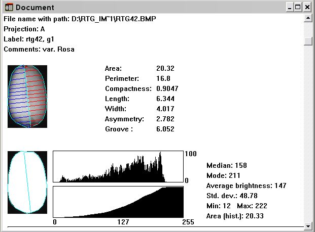
details in [4].A Complete Gradient Clustering Algorithm for Features Analysis of X-ray Images 5 3 Materials and methods The proposed algorithm has been tested on a real data set of grains. Studies were conducted using combine harvested wheat grain originating from experimental fields, explored at the Institute of Agrophysics of the Polish Academy of Sciences in Lublin. The examined group comprised kernels belonging to three different va- rieties of wheat: Kama, Rosa and Canadian, 70 elements each, randomly selected for the experiment. Visualization of the internal kernel structure was detected us- ing a soft X-ray technique. The images were recorded on 13x18 cm X-ray KODAK plates. Figure 1 presents the X-ray images of these kernels. Fig. 1 X-ray photograms (18x13cm) of kernels The X-ray photograms were scanned using the Epson Perfection V700 table photo-scanner with a built-in transparency adapter, 600 dpi resolution and 8 bit gray scale levels. Analysis procedures of obtained bitmap graphics files were based on the computer software package GRAINS, specially developed for X-ray diagnostic of wheat kernels [7]. To construct the data, seven geometric parameters of grains: area A [mm2 ], perimeter P [m], compactness C = 4πA/P2 , length of kernel [mm], width of kernel [mm], asymmetry coefficient and length of kernel groove [mm] were measured from a total of 210 samples (see Figure 2). In our study, the data was reduced to be two-dimensional after applying the prin- cipal component analysis to validate the results visually. All calculations were carried out on an IBM/PC compatible computer with the Windows XP operation system, and all programs were developed in Borland C++ Builder Environment.
6                                                                        M. Charytanowicz et al.

Fig. 2 Document window with geometric parameters of a kernel and statistical parameters of its
image

4 Results and discussion

The dataset consists of 210 kernels belonging to three wheat varieties, 70 elements
each, characterized by 7 geometric features, all of these real-valued continuous. The
data’s projection on the axes of the two greatest principal components is presented
in Figure 3 with wheat varieties being distincted symbolically.

Fig. 3 Wheat varieties data set on the axes of the two greatest principal components: (◦) the Rosa
wheat variety, (×) the Kama wheat variety, (ut) the Canadian wheat variety
A Complete Gradient Clustering Algorithm for Features Analysis of X-ray Images            7

   All samples are labeled by numbers: 1-70 for the Kama wheat variety, 71-140
for the Rosa wheat variety, and 141-210 for the Canadian wheat variety. The CGCA
created three clusters corresponding to Rosa, Kama, and Canadian varieties, con-
taining 69, 65, and 76 grains respectively. Thus the samples 9, 38, which belong to
the Kama wheat variety are incorrectly grouped into the cluster associated with the
Rosa wheat variety. What is more, the samples 125, 136, 139, which belong to the
Rosa wheat variety, and the samples 166, 200, 202, which belong to the Canadian
wheat variety are wrongly classified into the cluster associated with the Kama wheat
variety. In addition, the samples 20, 27, 28, 30, 40, 60, 61, 64, 70, which belong to
the Kama wheat variety are wrongly classified into the cluster associated with the
Canadian wheat variety.
   Clustering results, containing numbers of grains classified properly and numbers
of grains classified wrongly into clusters associated with Rosa, Kama, and Canadian
varieties, are shown in Table 1.

Table 1 Clustering results of the Complete Gradient Clustering Algorithm and K-Means Algo-
rithm for the wheat varieties data set
              Complete Gradient Clustering Algorithm    K-Means Clustering Algorithm
 Clusters     Correct       Incorrect    Total          Correct       Incorrect   Total
 Rosa         67            2            69             66            2           68
 Kama         59            6            65             65            12          77
 Canadian     67            9            76             62            3           65

   According to the results of the CGCA, out of 70 kernels of the Rosa wheat vari-
ety, 67 was classified properly. Only 2 of the Kama variety were classified wrongly
as the Rosa variety. These frequencies are equal 66 and 2 respectively if K-means
algorithm is used. The Rosa variety is best recognized using both techniques.
   For the other two varieties, the CGCA created clusters containing 65 elements
(Kama) and 76 elements (Canadian). In regard to the Kama variety, 59 kernels were
classified correctly, while 6 of the other varieties were incorrectable identified as
the Kama variety. For the Canadian variety, 67 kernels were correctly identified
and 9 kernels of the Kama variety were wrongly identified as the Canadian variety.
Results obtained using K-means algorithm were the following: the Kama variety:
out of 77 kernels, 65 were correctly identified and 12 incorrectly identified; the
Canadian variety: our of 65 kernels, 62 were correctly identified and 3 incorrectly
identified. This implies, that Kama and Canadian varieties are similar with respect
to geometric parameters.
   The percentages of correctness of both methods are summarized in Table 2. The
proposed algorithm achieved accuracy of about 96% for the Rosa wheat variety,
84% for the Kama wheat variety, and 96% for the Canadian wheat variety. In com-
parison, K-means algorithm achieved accuracy of about 94%, 93%, and 89% re-
spectively.
8 M. Charytanowicz et al.
Table 2 Comparison of performance of the Complete Gradient Clustering Algorithm and K-Means
Algorithm for the wheat varieties data set, correctness percentages are reported
Complete Gradient Clustering Algorithm K-Means Clustering Algorithm
Wheat Varieties Correctness % Correctness %
Rosa 96 94
Kama 84 93
Canadian 96 89
5 Conclusions
The proposed clustering algorithm, based on kernel estimator methodology, is ex-
pected to be an effective technique for forming proper categories of wheat. It be-
haves equally or better than the classical K-means algorithm. Moreover, the data
reduced after applying the principal component analysis, contained apparent clus-
tering structures according to their classes. Both algorithms performed well and the
percentages of correctness were comparable. The amount of 193 grains, giving al-
most 92% of the total, was classified properly. The wheat varieties used in the study
showed differences in geometric parameters. The Rosa variety is better recognized,
whilst Kama variety and Canadian variety are less successfully differentiated. Fur-
ther research is needed on grain geometric parameters and these ability to identify
wheat kernels.
References
1. Fukunaga K, Hostetler L D (1975) The estimation of the gradient of a density function, with
applications in Pattern Recognition. IEEE Transactions on Information Theory 21:32-40
2. Kowalski P, Łukasik S, Charytanowicz M, Kulczycki P (2008) Data-Driven Fuzzy Modeling
and Control with Kernel Density Based Clustering Technique. Polish Journal of Environmen-
tal Studies 17:83-87
3. Kulczycki P (2008) Kernel estimators in industrial applications. In Prasad B (ed) Soft Com-
puting Applications in Industry. Springer-Verlag, Berlin
4. Kulczycki P, Charytanowicz M (2010) A Complete gradient clustering algorithm formed with
kernel estimators. Int. J. Appl. Comput. Sci., in press
5. Mirkin B (2005) Clustering for Data Mining: A Data Recovery Approach. Chapman and
Hall/CRC, New York
6. Silverman B W (1986) Density Estimation for Statistics and Data Analysis. Chapman and
Hall, London
7. Strumiłło A, Niewczas J, Szczypiński P, Makowski P, Woźniak W (1999) Computer system
for analysis of X-ray imges of wheat grains. Int. Agrophysics 13:133-140You can also read