A Formal Safety Characterization of Advanced Driver Assist Systems in the Car-Following Regime with Scenario-Sampling ??
←
→
Page content transcription
If your browser does not render page correctly, please read the page content below
A Formal Safety Characterization of
                                                                            Advanced Driver Assist Systems in the
                                                                                 Car-Following Regime with
                                                                                    Scenario-Sampling ??
                                                                                Bowen Weng+ ∗ Minghao Zhu+ ∗ Keith Redmill ∗
                                                                        ∗
                                                                            Department of Electrical and Computer Engineering at Ohio State
                                                                               University, OH, 43210 USA (e-mail: weng.172@osu.edu,
                                                                                       zhu.1385@osu.edu, redmill.1@osu.edu).
arXiv:2202.08935v2 [cs.RO] 23 May 2022

                                                        Abstract: The capability to follow a lead-vehicle and avoid rear-end collisions is one of the
                                                        most important functionalities for human drivers and various Advanced Driver Assist Systems
                                                        (ADAS). Existing safety performance justifications of car-following systems either rely on simple
                                                        concrete scenarios with biased surrogate metrics or require a significantly long driving distance
                                                        for risk observation and inference. In this paper, we propose a guaranteed unbiased and sampling
                                                        efficient scenario-based safety evaluation framework inspired by previous work on δ-almost safe
                                                        set quantification. The proposal characterizes the complete safety performance of the test subject
                                                        in the car-following regime. The performance of the proposed method is also demonstrated in
                                                        challenging cases including some widely adopted car-following decision-making modules and the
                                                        commercially available Openpilot driving stack by CommaAI.

                                                        Keywords: Test and Validation, Scenario Sampling, Set Invariance, Advanced Driver Assist
                                                        Systems.

                                                               1. INTRODUCTION                              improve the sampling efficiency. However, the required
                                                                                                            testing effort is still too significant to be widely appli-
                                         The car-to-car rear-end collision has been the most com-           cable in practice. The naturalistic driving environment
                                         mon crash type in the U.S. for decades. Various Advanced           is not necessarily unchanged and may vary significantly
                                         Driver Assist Systems (ADAS) have been developed and               from time to time. For those importance sampling based
                                         deployed to help mitigate the read-end collision risk, in-         variants, the importance function estimate was developed
                                         cluding crash-imminent braking (CIB), autonomous emer-             with various heuristics, making it difficult to justify its
                                         gency braking (AEB), traffic jam assist (TJA), adaptive            accuracy. Also, as reported by Weng et al. (2021a), such a
                                         cruise control (ACC), and pedestrian crash avoidance miti-         statistical inference method occurs in an implicitly defined
                                         gation (PCAM). In this paper, we are primarily interested          operable domain with the tendency to over-estimate the
                                         in vehicle following ADAS, which cover a large portion             risk. Finally, a simple scalar measure of risk is not neces-
                                         of the currently available ADAS. We assume the Subject             sarily sufficient to justify the complete safety performance
                                         Vehicle (SV) is sufficiently well-performed in other oper-         of an SV.
                                         ational modules, such as lane-keeping. This is a common            The dominant approach adopted by most existing regula-
                                         assumption and is feasible to achieve in the practice of           tory and standards follows the scenario-based test where
                                         ADAS tests. We also emphasize that the proposed ap-                the SV is deployed as a black-box system (uncontrol-
                                         proach is applicable to evaluate other ADAS modules, such          lable and partially observable) in a testing case with the
                                         as the Lane-Keeping Assist System (LKAS), yet details are          lead vehicle following a certain prescribed control policy.
                                         beyond the scope of this paper.                                    The common practice in this case presents a finite set
                                         The safety evaluation of an ADAS-equipped SV in the car-           of concrete scenarios and analyzes the testing outcome
                                         following and rear-end collision avoidance regime seeks to         through an independent safety metric (i.e. the metric is
                                         characterize the SV’s safety performance against station-          computed independently from the test execution and data
                                         ary/moving vehicles in the front of the SV within the same         acquisition, and the testing data is presented as it stands).
                                         lane, or along the SV’s current trajectory. One common             Some commonly observed concrete scenarios in the rear-
                                         testing approach is to observe the SV’s performance in the         end collision avoidance regime include the car-to-car lead
                                         real-world or simulated naturalistic driving environment           vehicle braking in Forkenbrock and Snyder (2015), the
                                         for a sufficiently long driving distance. One then observes        suddenly revealed stationary vehicle (SRSV) and the lead
                                         or infers the collision rate estimate. This is formally known      vehicle lane change and brake (LVLCB) in Rao et al.
                                         as the Monte-Carlo sampling, with other importance-                (2019), also known as the frontal cut-in scenario, to name
                                         sampling based variants from Zhao et al. (2017) that help          a few. The testing is mostly performed in a real-word prov-
                                         1 + These
                                                                                                            ing grounds with a certain strikable target that emulates
                                                     authors contributed equally.
the motion and the appearance of a lead vehicle. Some 2.1 δ-Almost Safe Set
also execute the test in a hardware-in-the-loop fashion
such as the augmented scenes by Feng et al. (2020). The The following definition is adapted from Weng et al.
results are then analyzed using an added metric, such (2021c,b).
as the observed collision rate, time-to-collision violation Definition 1. (δ-Covering Set) Give a compact set X ⊂
(TTCV) by Wishart et al. (2020), and other surrogate Rn for some n ∈ Z and δ ∈ Rn . For any x ∈ X , let
measures summarized in Wang et al. (2021). Note that Nδ (x) be the δ-neighbourhood of x, i.e., ∀x0 ∈ Nδ (x), |x −
this is also the testing approach adopted by many regula- x0 | ≤ δ. We claim that ΦX δ is a δ-covering set of X
tory standards such as the Europe NCAP by EuroNCAP if for some k ∈ Z and xi ∈ X , i = 1, . . . , k, we have
(2019). However, as reported by Weng et al. (2021c), the ΦX
S X
δ = i∈{1,...,k} Nδ (xi ) ⊇ X and Φσ = {xi }i∈{1,...,k} ⊆
set of concrete scenarios has very poor coverage of the
SV’s operational domain and is not of sufficient risk. The X . Furthermore, ΦX X
σ are centroids of Φδ .
safety metrics are mostly biased and fail to arrive at a
Recall C is the set of failure states (e.g. collisions). The
consensus agreement and make a fair comparison among
following definition formally characterizes the notion of the
various SVs as shown in Weng (2021). The approach is
SV being “almost” safe in a certain set.
also fundamentally problematic if the underlying system is
stochastic which is a common phenomena in practice, and Definition 2. (δ-Almost Safe Set) Given the system
has been further enhanced as more learning-based methods dynamics (1), ∈ (0, 1], δ ∈ Rn , Φ ⊆ S. The set Φ is δ-
are involved in perception and decision-making modules. almost safe for the system (1) if there exists a δ-covering
set Φδ of Φ with Φσ such that Φδ ∩ C = ∅ and
In this paper, we propose a scenario-sampling framework
built on the Synchronous Pruning and Exploration (SPE) P ∀s ∈ Φσ , ∀ω ∈ W : f (s; ω) 6∈ Φδ ≤ . (2)
for safe set quantification in Weng et al. (2021c) with var-
ious improvements dedicated to the car-following regime It is immediate from the above definition that limδ→0 ΦX δ =
tests in practice. The basic idea of the proposed framework X . Also note that as tends to zero, the δ-almost safe set
seeks to characterize the safe operational design domain becomes an absolutely safe δ-covering set. To adapt the
(ODD) of the SV in the car-following regime through above definitions to the application of car-following regime
repeatedly sampling runs of scenarios in a guided manner. safety analysis, we shall first characterize the car-following
With a certain desired confidence level, one can then claim scenario in the form of (1).
at what states the SV is potentially safe and how safe
the SV is within the derived set of states. The proposed 2.2 The Scenario-based Car-Following System
method is further demonstrated in Section 4, where it is
shown capable of capturing various subtle safety properties In this paper, we consider the following system to formu-
and insights of widely adopted car-following models in late the interactive motion between a Subject Vehicle (SV)
both academic research as well as commercially available follower and a leading Principal Other Vehicle (POV) in
ADAS products in practice. The studied ADAS are more the front sharing the same lane with the SV:
realistic and difficult to evaluate than some of the previous
work by Fan et al. (2017) and Zhao et al. (2016). To the s(t + 1) = fs (s(t), u(t); ωs (t)). (3)
best of knowledge, many of the obtained properties have The state s = [d, v0 , v1 ] ∈ S ⊂ R3≥0 , where d ∈ [0, ∞)
never been captured by existing work in the field. denotes the distance headway (simplified as headway or
Notation: The set of real and positive real numbers are DHW in this paper) between the two vehicles, v0 ∈
denoted by R and R>0 respectively. Z denotes the set [0, vmax ] and v1 ∈ [0, vmax ] denote the longitudinal velocity
of all positive integers and ZN = {1, . . . , N }. |X | is the of the SV follower and the lead POV, respectively. In
cardinality of the set X . practice, significantly large d is not of safety concern,
hence the upper bound of d is often replaced with a
2. PRELIMINARIES AND PROBLEM sufficiently large value dmax ∈ R>0 . Other disturbances
FORMULATION and uncertainties are denoted as ωs ∈ Ws , which could
involve environmental features (e.g. weather condition
and road surface friction), infrastructure information (e.g.
Consider the general discrete-time system dynamics
road curvature, road gradient, and speed limit), other
s(t + 1) = f (s(t); ω(t)) (1) kinematic and dynamic features (e.g. lateral offset between
with state s ∈ S ⊆ Rn , uncertainties and disturbances the vehicles and acceleration status of vehicles), other road
ω ∈ W ∈ Rw , for some n, w ∈ Z. Let C ⊂ S denote the set users (e.g. pedestrian, cyclist, and other vehicles), planning
of failure states. Intuitively, for the system (1) to remain parameters (e.g., free-traffic speed), and measurement
statistically safe, there should exist S ∗ ⊂ S, S ∗ ∩ C = ∅ error, to name a few. As also discussed by Weng et al.
and all trajectories initialized in S ∗ remain inside S ∗ with (2021a), the state s and some of the uncertainties ωs may
high probability. The safety performance justification then be interchangeable depending on the particular feature’s
seeks to characterize the set S ∗ . In practice, S ∗ could be observability and how important it is in determining
non-convex, non-unique, and of other complex structures, safety related properties. For example, EuroNCAP (2019)
leading to various challenges for accurate characterization, consider the lateral offset between vehicles as an important
statistically or deterministically. In this paper, we adopt feature that affects the performance of SV, leading to an
the δ-almost safe set based methods from Weng et al. extra dimension added to the state s. The action u ∈ U ⊂
(2021b). Some important definitions and theorems are R represents the control input of the lead POV, such as
revisited in the following sub-section. the desired velocity and the commanded acceleration. Notethat the SV is the test subject in the testing content, following scenario system in the form of (1). Let S0 ⊆ S
thus it is an uncontrollable and (partially) observable be the sup-set of all safe sub-sets in S. The car-following
black-box system (see Remark 3 in Weng et al. (2021c)). safe set quantification problem seeks to find a scenario-
Furthermore, the action u is typically determined by a sampling algorithm ALG : S ×(0, 1]×(0, 1]×Rn → S, such
certain feedback control policy that with confidence level at least 1 − β, ALG(S0 , , δ, β)
u = π(s, ωs ; ωu ), (4) is an δ-almost safe set for (1).
with s, ωs the same with what we have defined above, The previous work by Weng et al. (2021c) has already
and the uncertainties ωu ∈ Wu . Intuitively, the policy π presented various algorithms that provably solve the above
describes the lead POV driving behavior. In the scenario- problem with a primary focus on completeness and asymp-
based safety evaluation regime, the testing policy is a totic optimality properties. Such properties occur as the
given function. As a result, composing (3) with (4) we number of samples tends to infinity which leads to a signifi-
have the exact system dynamics of (1) with n = 3. The cant amount of samples required in practice. In this paper,
disturbances and uncertainties ω ∈ W is jointly affected we propose a modified version of the Synchronous Pruning
by s, ωs in (3) and ωu in (4). In practice, the scenario and Exploration for safe set quantification by Weng et al.
system may not necessarily exhibit the Markov Decision (2021c) with a specific focus on the car-following regime.
Process (MDP) nature induced by (1) as the next-step This leads to a theoretically sound and practically feasible
state may be dependent upon not only the current state, safe set quantification solution as we shall see in the next
but also a series of historic observations. One can extend two sections.
the state space to involve those observations, yet the state
space complexity will also increase significantly. In the We conclude this section by addressing the following
particular car-following domain studied by this paper, assumption and justifying its practical feasibility.
we argue that the capability of SV taking advantage of Assumption 1. Given the state space S, the set of failure
historical information, if applicable, would only make a states C, and the system (1), we assume that the run of
better safety performance. As a result, the safety property scenario can be initialized from any s ∈ S \ C.
obtained from system (1) still remains as the worst-case
justification. In practice, if one can control the engagement of the sub-
ject ADAS sufficiently accurately, the above assumption is
A run of a test scenario, RS(s0 , K) (K ∈ Z, K ≥ 2), naturally feasible, such as the test protocol by EuroNCAP
thus starts from a certain state initialization s0 ∈ S, (2019). On the other hand, if the ADAS is expected to
consecutively collects a set of states admitting the system engage before triggering the test, the accurate initializa-
dynamics (1), and terminates either when encountering a tion becomes more difficult at some states. In this case,
failure event (e.g., collision) or the K-th step of observation the above assumption is easy to achieve mostly at the
is reached. If f is explicitly known or approximately control equilibrium sub-set of S. For example, v0 = v1
characterized, one can execute the test scenario and collect for some d ∈ R>0 , which denotes the steady-state car-
data through computer simulations. On the other hand, following scene. This is also the initialization condition
the scenario-based test can also be performed in real-world adopted by Forkenbrock and Snyder (2015). Some non-
testing proving ground with f implicitly induced. control equilibrium states can be initialized through cus-
The standard scenario-based safety evaluation methods tomized scenes. For example, in the LVLCB test from the
(e.g. NCAP EuroNCAP (2019) and NHTSA guidelines NHTSA report by Rao et al. (2019), the lead-vehicle on the
in Forkenbrock and Snyder (2015); Rao et al. (2019)) side lane can choose to perform a lane change at any speed
specify the s0 based on expert-knowledge and real-world with any headway, which has the potential to initialize
crash database. The test policy π(·) is typically presented some non-control equilibrium states such as when v0
v1 .
as a deterministic function with constant deceleration Note that even with the above techniques, some states are
magnitude (e.g. π(s) = −6m/s2 , ∀s ∈ S in some of the car- still difficult to initialize, such as v0
v1, d = 0. However,
to-car AEB cases). In this paper, we adopt a similar design those difficult-to-achieve initialization states are typically
of π(·) used by the above mentioned standardized tests of obvious high-risk, thus they may not need to be tested
(i.e., the lead POV executes the braking maneuver at a anyway, as we shall see in Section 4.
constant deceleration rate). This evaluates the SV’s safety
performance in a more adversarial environment than the 3. MAIN METHOD
naturalistic driving environment. We also emphasize that
the proposed method does not rely on a particular testing To solve Problem 1, the overall algorithm follows a two-
policy, and will generalize easily to other testing policies, step procedure. First, one continuously constructs a can-
such as those emulating naturalistic driving behaviors didate set as more runs of scenarios are collected through
in Zhao et al. (2016). scenario sampling. Second, as the constructed set becomes
close to the actual almost safe set, one should observe a
2.3 The Almost Safe Set Quantification Problem sufficiently large number of runs of scenarios that start
from and remain inside the candidate set. For the second
Let a scenario-sampling algorithm consecutively sample step, the sampling sufficiency is justified by the following
runs of scenarios on S following the system dynamics (1). theorem.
We are now ready to present the car-following safe set Theorem 1. (δ-Almost Safe Set Validation) Given
quantification problem as follows. the system dynamics (1), ∈ (0, 1], β ∈ (0, 1], δ ∈ Rn ,
Problem 1. Given δ ∈ Rn , ∈ (0, 1], β(0, 1], a testing Φ ⊆ S, and the corresponding δ-covering set Φδ with
policy π(·) in the form of (4), and the corresponding car- centroids Φσ defined by Definition 1. Consider N runsof scenarios, {RS i (s0 , K)}i=1,...,N (K ∈ Z, K ≥ 2), with Algorithm 1 Car-following Safe Set Quantification
the state initialization of each run being i.i.d. w.r.t. the
1: Input: Initial set S0 ⊆ S, collision set C, ∈ (0, 1],
underlying distribution on Φσ . The set Φ is the δ-almost
β ∈ (0, 1], trajectory horizon K.
safe set for (1) with confidence level at least 1 − β if
SN ln β
2: Initialize: The δ-covering set of S0 , Φδ , and cen-
i=1 RS i (s0 , K) ⊆ Φδ ∩ C = ∅ and N ≥ ln (1−) . troids Φσ by Definition 1, the state graph Gσ =
(Φσ , Eσ ), Eσ = ∅ ⊂ S 2 , the unsafe state graph Gu =
That is, under the given conditions, if one consecutively (Du , Eu ), Du = ∅ ⊂ S, Eu = ∅ ⊂ S 2 , prioritized replay
observes ln ln β
(1−) runs of scenarios remaining inside Φδ , one buffer B = ∅, N=0.
ln β
then have the confidence level at least 1 − β to claim that 3: While N < ln (1−) :
the probability for any trajectory starting from Φσ to leave 4: If B = ∅
Φδ is less than , i.e., the SV is δ-almost safe in the set 5: s0 ∼ P (Φσ )
Φ. One can refer to Weng et al. (2021c) for the proof of 6: Else
Theorem 1. 7: sb = B.pop(), s0 = Φσ .nearest(sb )
The proposed algorithm to solve Problem 1 is presented 8: End If
as Algorithm 1 taking advantage of the Theorem 1. Note 9: Get T = RS(s0 , K)
that pop, reachable, nearest, remove, and append are 10: If T ∩ C = 6 ∅
all notional functions. X .pop() returns a point x ∈ X 11: For i in Z|T |−1 do
and removes it from the set. reachable(s, G) returns 12: B.append(T [i])
all vertices on the graph G that connects, directly and 13: For s in Reachable(T [i], Gσ ) do
indirectly, to the point s through a depth-first-search 14: Φσ .remove(s)
routine (see Weng (2022)). X .nearest(x) returns the 15: Eu .append((T [i], T [i + 1]))
nearest point to x in X in terms of `2 -norm distance. The 16: End For
commands remove and append simply remove a point from 17: B.append(T [i + 1])
or add a point to the given set, respectively. 18: End For
19: N =0
Overall, Algorithm 1 consists of four major steps. The 20: Else
initialization step (line 2) configures two graphs, Gσ and 21: s̄ = s0 , Ns = |Φσ |
Gu , that are intended to contain potentially safe and ob- 22: For i in {2, . . . , |T |} do
served unsafe states and transitions, respectively, through 23: If T [i] ∈/ Φδ
scenario-sampling. The sampling step (line 4-7) takes a 24: Eσ .append((s̄, T [i]))
i.i.d. sample by Theorem 1 if the prioritized replay buffer 25: s̄ = T [i]
B is empty. Otherwise, i.e. when some unsafe states have 26: End If
been observed and added to B at line 12, it prioritizes 27: End For
sampling points in Φσ that are close to the points in B 28: If Ns = |Φσ | and B = ∅
as they are intuitively of higher-risk. Such a sampling 29: N+ = 1
heuristic will not jeopardize the claimed property in The- 30: Else
orem 1 for set validation, as B will be empty eventually, 31: N =0
but will accelerate the convergence to a sufficiently almost 32: End If
safe set as unsafe points are removed more frequently. 33: End If
The third important stage happens at line 10-19. When 34: Output: Φδ
a sampled run of a scenario is observed to converge to
C, any reachable states to the points in the collected run
are removed from Φσ . On the other hand (line 21-32), one 4. CASE STUDIES
either adds an uncovered point to the covering set (line
23-25) or consecutively observes N runs of scenarios that To demonstrate the performance of the proposed Algo-
remain inside Φδ to claim the δ-almost safe property. rithm 1, we start with examples of safety evaluations of
The proposed algorithm differs from the SPE for safe set deterministic decision-making systems where the percep-
quantification in Weng et al. (2021c) in two main ways, tion and the control modules are both sufficiently accurate.
the use of prioritized sampling with a replay buffer and We then move to an end-to-end case study taking the Com-
the removed stage of δ decay. The prioritized sampling maAI’s Openpilot by Shihadeh et al. (2018) as an example
with a replay buffer is a heuristic approach that improves which involves a neural-network based perception module,
the convergence rate to a potentially almost safe set. camera-radar sensor fusion, model-based decision-making,
The fixed choice of δ and compromises the probabilistic and control modules. The source code for Algorithm 1 in
completeness of the algorithm in return for practical Python can be found at Weng (2022).
feasibility with improved sampling efficiency (as we shall
4.1 Decision-Making Safety Evaluation
also see empirically in Section 4). One can always re-
obtain the completeness and optimality properties, or
We consider two classes of decision making systems in
at least achieve an appropriate level of compromisation,
this section. The first is a combination of ACC and AEB
by configuring δ and to be arbitrarily close to zero,
(ACC-AEB) first introduced by Zhao et al. (2016). When
yet the number of required samples might also increase
the perceived time-to-collision value is greater than a pre-
dramatically.
determined threshold, the ACC module is engaged as a
discrete Proportional-Integral (PI) controller to achieveFig. 1. Some δ-almost safe sets obtained for the car-following case
study with various decision-making modules ( = 0.01, β =
0.001): (a) ACC-AEB with δ = [10, 2, 2], (b) ACC-AEB with
δ = [10, 6, 6], (c) N IDM with δ = [10, 6, 6], (d) M IDM with
δ = [10, 6, 6], (e) H IDM with δ = [10, 6, 6]. Fig. 2. M IDM’s commanded acceleration inputs for a group of
Table 1. The safety evaluation results for various (v0 , v1 ) pairs at 40-meter headway in the car-following scenario.
decision-making modules in the car-following case (β =
0.001, δ = [10, 6, 6]) and Openpilot presented in Sec- representing a subspace slicing of a certain headway value.
tion 4.2 (β = 0.001, δ = [3, 3, 3]). Intuitively, the size of the safe set increases as the lead-
SV S0 scenario runs collision runs IoU
POV becomes further away, since the state is of lower-
ACC-AEB S 0.1 867.5 ± 281.2 268.3 ± 34.5 0.915 risk as the lead-POV operates at a higher speed than the
S 0.01 1912.6 ± 146.4 185.4 ± 1.4 1.000 SV follower. This is mostly correct if one observes the
H IDM S 0.1 194.2 ± 14.6 40.7 ± 3.2 0.965 IDM cases where M IDM has the smallest almost safe set
S 0.01 1376.0 ± 182.1 49.0 ± 0.0 1.000
N IDM S 0.1 368.5 ± 95.0 69.6 ± 4.4 0.952
and H IDM has the largest almost safe set, which aligns
S 0.01 1628.8 ± 266.3 74.6 ± 0.8 0.998 with the underlying configurations of M IDM having the
Fig 1e 0.01 1578.6 ± 220.1 26 ± 0.0 1.000 lowest braking capability and H IDM having the strongest
M IDM S 0.1 830.9 ± 88.3 155.6 ± 3.7 0.956 braking capability among all tested IDMs.
S 0.01 1892.6 ± 237.5 161.0 ± 0.0 1.000
Fig 1e 0.01 1731.4 ± 125.5 112.0 ± 0.0 1.000 However, for most of the subplots in the ACC-AEB case,
Openpilot S 0.1 704.2 ± 54.3 141.8 ± 3.4 0.897
especially those with large headway values, one exhibits
a non-convex almost safe set with a white notch, which
a desired time headway. Otherwise, the AEB module ex-
indicates some unsafe states even when the headway is
tracted from a 2011 Volvo V60 is active. The ACC-AEB
sufficiently large. This is mainly due to the ACC design
module takes the same hyper-parameters and configura- nature where one tends to reach the free-traffic speed
tion as Zhao et al. (2016), having a maximum braking aggressively when the headway value is high, v0 thus
capability of −10m/s2 subject to a deceleration change increases, ending up in a certain unsafe state. For a similar
rate limit of −16m/s3 . The second decision-making module cause, ACC-AEB also fails all of the CCRb and CCRm
studied by this section is the Intelligent Driving Model tests in Fig 6. As a result, if one considers the free-
(IDM) in Treiber and Kesting (2013), which is a widely traffic speed as an observable state and expands the S
adopted car-following model in the field. Note that we to be of dimension four, the corresponding almost safe
have created three IDM variants based on the maxi- set will also change w.r.t. the desired velocity. A detailed
mum brake control capability. In particular, we have the analysis regarding this variant, and possibly other variants
normal-brake IDM (N IDM) with −5m/s2 , the mild-brake considering different added features, are of future interest.
IDM (M IDM) with −3m/s2 , and the hard-brake IDM
(H IDM) with −7m/s2 . Other IDM parameters include Returning to the notch observation, why isn’t a similar
the minimum safe distance (2 m), maximum acceleration shape showing up on any of the IDM variants in Fig 1?
(0.73m/s2 ), comfortable deceleration (1.67m/s2 ), safe time This is because the IDM is primarily a car-following model
headway (2 s), exponent of acceleration (4), and vehicle and may not necessarily exhibit expected behaviors out-
length (4 m). Unless mentioned otherwise, we consider the side the normal car-following work domain. For example,
state space S with the headway d ∈ [0, 100] m, SV speed Fig 2 illustrates the M IDM’s acceleration outputs for a
v0 ∈ [0, 30] m/s, and lead POV speed v1 ∈ [0, 30] m/s. group of (v0 , v1 ) pairs with 40-meter headway. Note that at
Note that the collected run of a scenario might leave S with v0 = 12 m/s, v1 = 25 m/s, the M IDM decides to execute
a large headway value that is greater than the given upper maximum brake maneuver, rather than to accelerate to
bound (100 m), in which case, one shall either truncate track the desired speed. This leads to a utility performance
the trajectory or clip the headway value at the given degradation in terms of velocity tracking, but on the other
upper bound before proceeding to line 10 of Algorithm 1. hand, improves the safety performance against potential
The simulation of each run of scenario operates at 10 Hz rear-end collisions. Fundamentally speaking, the observed
with K = 300. The testing policy admits the form of phenomena is caused by a squared term associated with
π(s) = −5m/s2 , ∀s ∈ S. We also assume the free-traffic the (v0 − v1 ) term in the IDM formulation, the details are
speed to be 30 m/s. beyond the scope of this paper.
We execute Algorithm 1 for 10 times with 10 different Moreover, comparing Fig 1(a) and Fig 1(d), the ACC-
random seeds. The set of 10 seeds remains the same among AEB has a relatively larger safe set than M IDM when the
different SVs. Some of the obtained almost safe sets for headway value is small. As the headway value increases,
= 0.01, β = 0.001 are illustrated in Fig 1 for the the safe set of M IDM enlarges significantly and eventually
same seed. The three-dimensional safe set is illustrated out-performs ACC-AEB in terms of the safe set size. That
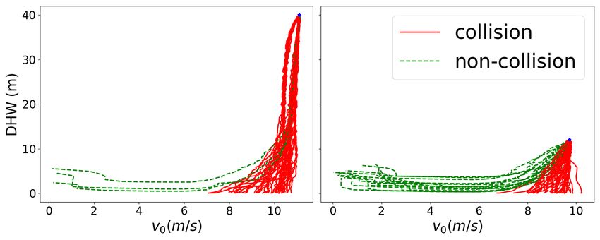
with a series of subplots on the (v0 , v1 ) domain, each is, the notion of “one vehicle being safer than the other”Fig. 3. Some δ-almost safe sets obtained for the car-following (a) ACC-AEB. (b) Openpilot.
case study with Openpilot for three different random seeds Fig. 4. The δ-almost safe sets ( = 0.01, β = 0.001) obtained for
can be problematic
( = as it is essentially a multi-dimensional
0.1, β = 0.001) ACC-AEB and Openpilot in a lead-obstacle scene where the
comparison. A similar point was also made by Weng lead-POV remains stationary for all time.
et al. (2021a) through observing real-world car-following
performance in the naturalistic driving environment. Such
a subtle safety characterization is difficult to obtain by
existing concrete scenario-based testing strategies such as
the NCAP AEB testing shown in Fig 6.
More detailed results regarding this case are listed in
Table 1. The “IoU” denotes the intersection-over-union
ratio of all obtained safe sets from different seeds w.r.t.
the same SV. It is clear that the higher the IoU value Fig. 5. The trajectories on the (v0 , d) domain of Openpilot tested
is, the more similar the obtained sets are among different in two standard NCAP Car-to-Car Rear moving scenarios.
For both scenarios, the lead POV remains at 20 km/h (5.56
seeds. Considering the studied decision-making modules in
m/s). All other parameters and environmental configurations
this section are both deterministic, the IoU value should remain identical among all test runs for the same initialization
converge to one for sufficiently small and β. This has condition. Within each subplot, Openpilot is enabled at the
been validated empirically by row 2, 4, 7, 9, and 10 in illustrated initialization state and both vehicles, unless specified
Table 1. We emphasize that even for the cases with IoU otherwise by the testing procedure, maintain at the steady-
values less than one, the results are not wrong, as the δ- state stage with zero acceleration.
almost safe set is simply not unique for the studied system. Openpilot in Carla, we use the Openpilot-Carla bridge
Also, note that if the set initialisation is not S0 but is provided by CommaAI as a foundation with added clus-
another set that is closer to the final almost safe set, one tered radar results for radar-camera fusion to enable the
should expect a smaller number of runs of scenarios and, ACC in Openpilot. The radar points clustering configu-
more importantly, a smaller number of runs of scenarios ration is identical to the work by Zhong et al. (2021).
with collisions, to converge to the desired outcome (e.g. The detailed implementation can be found at Zhu (2022).
comparing row 6 with row 7, and comparing row 9 with The state space S takes the configuration d ∈ [0, 30] m,
row 10 in Table 1). v0 ∈ [0, 15] m/s, and v1 ∈ [0, 15] m/s. The simulation of
Overall, the total number of runs of scenarios varies w.r.t. each run of scenario operates at 100 Hz with K = 500. The
the SV, the selected hyper-parameters (e.g. , β) and the free-traffic speed is 11.176 m/s (25 mph) if v0 (0) < 11.176
random seed, but remains below 2000 (i.e., less than 17- and v0 (0) otherwise, which is the default configuration of
hour (2000 runs of scenarios with at most 30 seconds for Openpilot.
each run) of actual scenario-running time excluding the Note that Openpilot is not designed for emergency col-
testing preparation and scenario restoration time). This is lision avoidance as suggested by CommaAI at Shihadeh
a slightly higher testing burden than the existing standards et al. (2018). It is primarily a car-following model. As
for the car-following regime but should still be considerred a result, an adversarial testing policy, such as the one
feasible in practice. One can improve the efficiency in com- adopted for the decision-making case, could lead to a very
puter simulations by executing multiple testing scenarios limited safe set. For example, as shown in Fig 4, if the
in parallel. Moreover, the testing effort may be further lead vehicle remains stationary (similar to the CCRs case
reduced for a smaller K, and the exploration regarding this by EuroNCAP (2019) and also included in Fig 6), the
direction is of future interest. More importantly, among Openpilot SV almost fails to avoid any rear-end collisions
the methods that are capable of providing similar theo- if v0 ≥ 4.5m/s. The Openpilot’s almost safe set is also
retical guarantees, the proposed solution appears to be significantly smaller than a regular almost safe set in cases
the most practical and is capable of capturing the subtle such as the one shown for ACC-AEB in Fig 4a. In this
differences among various SVs. For comparison, the impor- section, we admit the testing policy as π(s) = 0 m/s2 ,
tance sampling and Monte-Carlo sampling based methods which emulates the steady-state car-following situation.
reported by Zhao et al. (2017) require hundreds of millions
of test runs in simulation for safety evaluation with car- We execute Algorithm 1 for 5 times with 5 different
following maneuvers and only generate a risk estimate. random seeds. Some of the obtained almost safe sets for
= 0.1, β = 0.001 with three different seeds are illustrated
4.2 End-to-End Safety Evaluation in Fig 3. Other statistical properties are summarized
in the last row of Table 1. Note that the IoU rate in
For an end-to-end case study, we evaluate the CommaAI Table 1 is slightly smaller than the presented cases in
Openpilot’s safety performance in the car-following regime Section 4.1. This is mainly due to the fact that Openpilot
through simulation using the Carla simulator. To run the is fundamentally stochastic, as also illustrated by Fig 5Forkenbrock, G.J. and Snyder, A.S. (2015). NHTSA’s
2014 automatic emergency braking test track evalua-
tions. Technical report, National Highway Traffic Safety
Administration.
Rao, S.J., Forkenbrock, G.J., et al. (2019). Test procedures
traffic jam assist test development considerations. Tech-
nical report, United States. Department of Transporta-
tion. National Highway Traffic Safety Administration.
Shihadeh, A. et al. (2018). openpilot. https://github.
Fig. 6. The testing outcomes of all studied SVs in Section 4 with the com/commaai/openpilot.
standard NCAP car-to-car AEB testing procedure discussed Treiber, M. and Kesting, A. (2013). Traffic flow dynamics.
in EuroNCAP (2019). The procedure specifies 48 different Traffic Flow Dynamics: Data, Models and Simulation,
scenario configurations from three categories including the
Car-to-Car Rear stationary (CCRs), Car-to-Car Rear moving
Springer-Verlag Berlin Heidelberg.
(CCRm), and Car-to-Car Rear braking (CCRb), where the Wang, C., Xie, Y., Huang, H., and Liu, P. (2021). A re-
lower-case letter after CCR induces the lead-POV’s driving view of surrogate safety measures and their applications
behavior (staying stationary, moving at a constant velocity, or in connected and automated vehicles safety modeling.
braking to stop). Each deterministic decision-making module is Accident Analysis & Prevention, 157, 106157.
only tested once. The Openpilot enabled SV is tested with the Weng, B. (2021). A class of model predictive safety
same set of 48 scenarios for 10 times. The detailed parameters performance metrics for driving behavior evaluation.
related to the order of all testing cases can be found in In 2021 IEEE International Intelligent Transportation
“ncap bridge.py” at Zhu (2022). Systems Conference (ITSC), 180–187. doi:10.1109/
and Fig 6 where, starting from the same s0 , the Openpilot ITSC48978.2021.9565013.
enabled SV is shown capable of generating both safe and Weng, B. (2022). SDQ tools. https://gitlab.com/
collision outcomes. As a result, the almost safe set for Bobeye/sdq_tools.
Openpilot in the studied domain is fundamentally non- Weng, B., Capito, L., Ozguner, U., and Redmill, K.
unique, making it a particularly challenging case for many (2021a). A finite-sampling, operational domain specific,
existing scenario-based techniques and surrogate safety and provably unbiased connected and automated vehicle
metrics. As for the proposed method, the obtained safe set safety metric. arXiv preprint arXiv:2111.07769.
aligns with the claimed operational domain by CommaAI. Weng, B., Capito, L., Ozguner, U., and Redmill, K.
The SV remains safe with high probability when v0 ≥ v1 (2021b). A formal characterization of black-box sys-
regardless of the following distance. The size of the almost tem safety performance with scenario sampling. IEEE
safe set also increases as the headway value becomes larger. Robotics and Automation Letters. doi:10.1109/LRA.
2021.3122517.
Weng, B., Capito Ruiz, L.J., Ozguner, U., and Redmill,
5. CONCLUSION K. (2021c). Towards guaranteed safety assurance of
automated driving systems with scenario sampling: An
In this paper, we have presented a theoretically sound invariant set perspective. IEEE Transactions on Intel-
and sampling efficient scenario-sampling framework for the ligent Vehicles. doi:10.1109/TIV.2021.3117049.
safety performance evaluation of various car-following and Wishart, J., Como, S., Elli, M., Russo, B., Weast, J.,
rear-end collision avoidance systems. The performance of Altekar, N., James, E., and Chen, Y. (2020). Driving
the proposed method has been demonstrated empirically safety performance assessment metrics for ads-equipped
through a series of challenging cases. It is of future interest vehicles. SAE Technical Paper, 2(2020-01-1206).
to improve the completeness of the formulated scenario Zhao, D., Huang, X., Peng, H., Lam, H., and LeBlanc, D.J.
state space and develop more sampling-efficient safe set (2017). Accelerated evaluation of automated vehicles
quantification algorithms. The proposed method is also in car-following maneuvers. IEEE Transactions on
expected to generalize to the safety evaluation of other co- Intelligent Transportation Systems, 19(3), 733–744.
operative car-following systems and human drivers within Zhao, D., Lam, H., Peng, H., Bao, S., LeBlanc, D.J.,
the same operable domain. Nobukawa, K., and Pan, C.S. (2016). Accelerated evalu-
ation of automated vehicles safety in lane-change scenar-
REFERENCES ios based on importance sampling techniques. In IEEE
Transactions on Intelligent Transportation Systems, vol-
EuroNCAP (2019). European new car assessment pro- ume 18, 595–607. IEEE.
gramme (euro ncap) test protocol – AEB car-to-car Zhong, Z., Hu, Z., Guo, S., Zhang, X., Zhong, Z., and
systems. Technical report, The European New Car Ray, B. (2021). Detecting safety problems of multi-
Assessment Programme. sensor fusion in autonomous driving. arXiv preprint
Fan, C., Qi, B., Mitra, S., and Viswanathan, M. (2017). arXiv:2109.06404.
D ry vr: data-driven verification and compositional Zhu, M. (2022). Openpilot in Carla. https://github.
reasoning for automotive systems. In International com/pgchui/openpilot_in_carla.
Conference on Computer Aided Verification, 441–461.
Springer.
Feng, S., Feng, Y., Yan, X., Shen, S., Xu, S., and Liu, H.X.
(2020). Safety assessment of highly automated driving
systems in test tracks: a new framework. Accident
Analysis & Prevention, 144, 105664.You can also read