A least squares support vector regression for anisotropic diffusion filtering
←
→
Page content transcription
If your browser does not render page correctly, please read the page content below
A least squares support vector regression for
                                           anisotropic diffusion filtering

                                           Arsham Gholamzadeh Khoee · Kimia
                                           Mohammadi Mohammadi · Mostafa
                                           Jani · Kourosh Parand

                                           the date of receipt and acceptance should be inserted later
arXiv:2202.00595v1 [eess.SP] 30 Jan 2022

                                           Abstract Anisotropic diffusion filtering for signal smoothing as a low-pass fil-
                                           ter has the advantage of the edge-preserving, i.e., it does not affect the edges
                                           that contain more critical data than the other parts of the signal. In this
                                           paper, we present a numerical algorithm based on least squares support vec-
                                           tor regression by using Legendre orthogonal kernel with the discretization of
                                           the nonlinear diffusion problem in time by the Crank-Nicolson method. This
                                           method transforms the signal smoothing process into solving an optimization
                                           problem that can be solved by efficient numerical algorithms. In the final anal-
                                           ysis, we have reported some numerical experiments to show the effectiveness
                                           of the proposed machine learning based approach for signal smoothing.

                                           Keywords Anisotropic diffusion filtering · Least squares support vector
                                           regression · Signal smoothing · Crank-Nicolson · Nonlinear PDE.

                                           A. G. Khoee
                                           Department of Computer Science, School of Mathematics, Statistics, and Computer Science,
                                           University of Tehran, Tehran, Iran
                                           E-mail: arsham.khoee@ut.ac.ir
                                           K. M. Mohammadi
                                           Department of Computer Sciences, Shahid Beheshti University, G.C., Tehran, Iran
                                           E-mail: ki.mohammadimohammad@mail.sbu.ac.ir
                                           M. Jani
                                           Department of Computer Sciences, Shahid Beheshti University, G.C., Tehran, Iran
                                           E-mail: m jani@sbu.ac.ir
                                           K. Parand
                                           Department of Computer Sciences, Shahid Beheshti University, G.C., Tehran, Iran
                                           Department of Cognitive Modelling, Institute for Cognitive and Brain Sciences, Shahid
                                           Beheshti University, G.C, Tehran, Iran
                                           School of Computer Science, Institute for Research in Fundamental Sciences (IPM), Tehran,
                                           Iran
                                           E-mail: k parand@sbu.ac.ir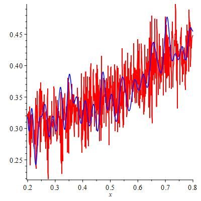
2                                                                 A. G. Khoee et al.

1 Introduction

Signal smoothing is generally about diminishing the high frequencies of a signal
in order to immediately discover the trend hidden in the signal and extract
some important features. It also makes the signal utilizable for further analysis.
For instance, the derivative of the signal may be required while the input signal
is not differentiable. In this situation, smoothing facilitates further analysis.
    Among various signal smoothing techniques, the anisotropic diffusion equa-
tion has found great importance, due to edge-preserving, denoising even the
smallest features of MR images, etc. in signal processing [1], as a fascinat-
ing technique in adaptive smoothing approaches. Adaptive smoothing meth-
ods are in contrast to the global smoothing methods, in which they do not
apply over smooth sharp edges and other valuable features of a signal [17].
Thus, anisotropic diffusion filtering has attracted considerable attention from
many researchers. At first, Witkin introduced the relation between the Gaus-
sian function and heat equation [31]. Later on, Perona and Malik found a
smoothing method based on a special nonlinear diffusion equation [21]. Also,
a time-fractional diffusion model is used for signal smoothing [12]. Moreover,
the diffusion filtering has been used for graph signals with an application in
recommendation systems [14]. It has also found applications for removing noise
in medical magnetic resonance images [13].
    Here, we present some preliminaries required in the rest of the paper.

1.1 The signal and the noise

In signal processing, noise is a destructive thing in analyzing, modifying, and
synthesizing signals. There are several techniques for omitting unwanted com-
ponents from a signal, but it is essential not to lose vital data after the smooth-
ing process and avoid reshaping. However, many of the existing techniques fail
to have this feature. We use anisotropic diffusion filtering, which is a well-
known technique for signal smoothing that performs better than other tech-
niques and preserves edges of the input signal.
    The quality of a signal is measured by the signal-to-noise ratio (SNR) that
represents the ratio of the signal power to the noise power, normally expressed
in decibels as:

                                               s2 (n)
                                           P
                                              n
                       SNR = 10 log P                   2
                                                          ,                     (1)
                                        n kf (n) − s(n)k

where s(n) is the smoothed signal and f (n) is the noisy signal.
    As a rule, a larger value of SNR means the power of the signal dominates
the power of noise. Note that the difference of the measures in decibel is equal
to the logarithm of the division.
    We demonstrate the isotropic and anisotropic diffusion equations in the
next section.
A LS-SVR for anisotropic diffusion filtering                                    3

1.2 Nonlinear diffusion equation and application in signal smoothing

Here, we describe the isotropic and anisotropic diffusion equation. The later,
also called the Perona–Malik equation, provides a technique to reduce noises
from a signal without dissolving edges and other significant features.
    The isotropic diffusion equation, as a heat equation, describes the temper-
ature changes in a material as time goes by. Isotropic diffusion equation, in
signal processing is equivalent to the heat equation as a partial differential
equation (PDE), given as:
                                  ∂u
                                      = k∇2 u,                              (2)
                                  ∂t
where u(x, t) represents the time evolution of a physical state such as the
temperature with the initial condition u(x, 0) as the input signal (with noise
added), and k controls the speed and spatial scale of changing the unit of
measure in time. In the heat equation, the coefficient depends on the thermal
conductivity of the material.
    Perona & Malik introduced anisotropic diffusion in which the heat flows
unevenly and force the diffusion process to contiguous homogeneous regions,
but not cross the region boundaries [20]. The formula is given as:
                              ∂u
                                 = ∇c · ∇u + c (x, t) ∆u,                     (3)
                              ∂t
where c refers to Perona-Malik coefficient which controls the rate of diffusion
and has been chosen as a function of the signal gradient so as to preserve
edges in the signal, Perona & Malik suggested two functions as the diffusion
coefficient:                                     2
                          c (k∇uk) = e−(k∇uk/K) ,                           (4)
and
                                                        1
                              c (k∇uk) =                      2 ,           (5)
                                                        k∇uk
                                               1+        K

in which the constant K adjusts the sensitivity to edges. Intuitively, a large
value of K leads back into an isotropic-like solution [21].
    Obviously, with a constant diffusion coefficient, the anisotropic diffusion is
reduced to the heat equation, which is referred to as isotropic diffusion, where
the heat flows evenly at all points of the material.
    The evolution of the noisy signal in the anisotropic diffusion process leads
to a smoothed signal.
    Now, we discuss the classical methods concerning signal smoothing.

1.3 Classic signal smoothing methods

Most of the classical smoothing algorithms are based on averaging, i.e. any
point of the signal is replaced by a weighted average of a subset of adjacent
points so providing a smooth result.
4                                                                       A. G. Khoee et al.

    The moving average algorithm is a fundamental smoothing algorithm, con-
verting an array of noisy data into an array of smoothed data. Assuming (yk )s
as a set of points of smoothed data set and n is the determined length of the
coefficient array, calculating points of the smoothed signal is done as follows:
                                             n
                                             X    yk+i
                                 (yk )s =              .                              (6)
                                            i=−n
                                                 2n +1

   In 1964, Savitzky and Golay [23] published a table of weighting coefficients,
derived by polynomial regression, in order to enhance edge-preserving. Their
work leads to another smoothing algorithm using a low degree polynomial.
Assuming (yk )s as a set of points of smoothed data set and Ai as a set of
particular weighting coefficients. The equation will be as follow:
                                     Pn
                                       i=−n Ai yk+i
                            (yk )s = P   n          .                        (7)
                                         i=−n Ai

Note that this technique is implemented on a nonsmooth-cure after a sampling
by function evaluation on some points.
     Another distinguished method is the Fourier Transform (FT) which manip-
ulates specific frequency components [10]. Any non-sinusoidal periodic signal
can be approximated to many discrete sinusoidal frequency elements. In fact,
by completely removing the high frequency elements, the smoothed signal will
be achieved. Despite some advantages, it is not computationally efficient.
     However, the most significant disadvantage of these classical methods is
still its weakness in preserving edges and peaks.
     We use a machine learning algorithm for numerical smoothing by nonlinear
diffusion equation which uses the Legendre polynomials as the kernel of LS-
SVR for our proposed approach. So we introduce Legendre polynomials in the
next section.

1.4 Legendre polynomials

Legendre polynomials are orthogonal polynomials with numerous applications,
e.g., in approximation theory and numerical integration [25]. They can be
generated recursively by the following relation [6]:

           (n + 1)Pn+1 (x) = (2n + 1)xPn (x) − nPn−1 (x),              n ≥ 1,         (8)

starting with
                               P0 (x) = 1,     P1 (x) = x.                            (9)
The next few Legendre polynomials are
                           1                           1
                P2 (x) =     (3x2 − 1),     P3 (x) =     (5x3 − 3x),   ....
                           2                           2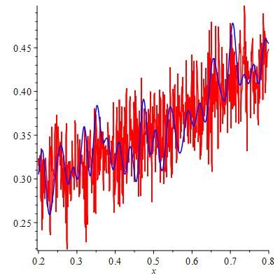
A LS-SVR for anisotropic diffusion filtering                                    5

   When used as a kernel of LS-SVR , the system of linear equations of the
LS-SVR has many properties including sparsity, low computational cost, and
some others, due to the orthogonality of this kernel.
   The Legendre polynomials are orthogonal over [−1, 1] with weight function
ω(x) = 1 as:

                       Z   1
                                                        2
                               Pn (x)Pm (x)ω(x)dx =          δmn ,          (10)
                         −1                           2n + 1

where δmn is the Kronecker delta.
   The symmetry contributes to the computational cost,

                    Pn (−x) = (−1)n Pn (x),      Pn (±1) = (±1)n .          (11)

Therefore, Pn (x) is an odd function, if n is odd. Furthermore, They are
bounded as:

                           |Pn (x)| ≤ 1,   ∀x ∈ [−1, 1], n ≥ 0,             (12)

      which avoids error propagation.
      These polynomials are the solution to Strum-Liouville differential equation
as:

                       ((1 − x2 )yn0 (x))0 + n(n + 1)yn (x) = 0,            (13)

with the solution yn (x) = Pn (x).
     The diffusion equation for smoothing is considered on the spatial domain
[0, 1], so we have used the shifted Legendre polynomials over [0, 1], given as:

                                   φn (x) = Pn (2x − 1)                     (14)

    In this paper, we present a numerical technique for signal smoothing based
on LS-SVR. We use the Legendre orthogonal polynomials as the kernel to re-
duce the computational complexity. To do so, first, a discretization in time
is carried out by implementing the Crank-Nicolson scheme. Then, the solu-
tion of the resulting boundary value problem is approximated in the LS-SVR
framework with two different approaches. The collocation points are used as
the training data.
    The rest of the paper is organized as follows. In section 2, we introduce
support vector machines, and least squares support vector regression (LS-
SVR). Section 3 is devoted to the main methodology and the explanation of
solving anisotropic diffusion equation with LS-SVR. Some numerical results
are reported in Section 4. The paper ends with some concluding remarks in
Section 5.
6                                                                 A. G. Khoee et al.

2 Support vector machines

Developing algorithms that lead to learning has long been an interdisciplinary
topic of research. It is proven that these algorithms can overcome many of the
weaknesses posed due to the deficiency of classic mathematical and statistical
approaches [3].
     Artificial Neural Networks (ANN) is known as one of the premier learning
approaches developed in the 1940s rest on the biological neuron system of
human brains. It found its widespread application almost four decades after
the invention of this method in pattern recognition ever since, due mainly
to its capability in extracting complex and non-linear relationships between
features of different systems. Though, over time it was determined that the
ANN could only perform accurately when a considerable amount of data is
available for training. It lacks generalization capacity in many instances, and
often a local optimal solution is given rather than a global most suitable result
[7].
     A new machine learning technique named support vector machines (SVM)
introduced by Vapnik [29] in the early 1990s as a non-linear solution for classi-
fication and regression problems. There are some reasons behind the authority
of the SVM in providing reliable outcomes. Main, its applicability is a subtle
issue that accounts for the name “support vector.” Not all training examples
are correspondingly relevant. Since the decision boundary only depends on
the training examples nearest to it, it suffices to define the underlying model
of SVM in terms of only those training examples. Those examples are called
support vectors [22]. It means that unlike the ANN, this method can give ac-
curate results with a limited number of available data. Also, unlike the ANN,
the probability of having a local optimal during the training process is highly
implausible when using the SVM due to having a quadratic programming
problem expressed in their mathematical model. Other, its robustness upon
the error of models. Unlike the ANN where the sum of squares error approach
is used to decrease the errors posed by outliers, the SVM considers the trade-off
parameter c and insensitivity parameter ε in the minimization problem which
is introduced in Section 2.1 in order to control the error of the classification or
the regression problem. Hence, the SVM can overthrow outliers by choosing
the proper values of depicted parameters in the minimization problem. Finally,
its computational performance and memory efficiency compared to the ANN
[30].
     A support vector machine seeks a precise hyperplane in a high dimensional
space that can be used for either classification or regression. Support vector
machines are supervised learning models used for linear and non-linear classi-
fication or regression analysis. The non-linear problem is performed using the
kernel-based function for mapping input into high dimensional feature space
[5].
     Their application can be found in pattern recognition [4], text classification
[27], anomaly detection [9], computational biology [24], speech recognition [8],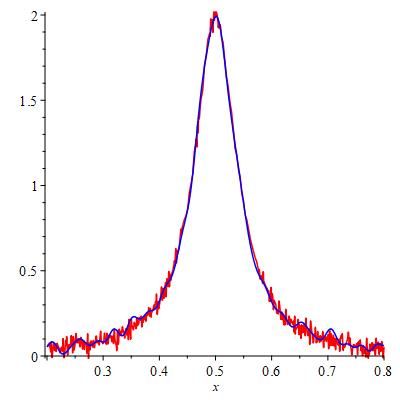
A LS-SVR for anisotropic diffusion filtering 7
adaptive NARMA-L2 controller for nonlinear systems [28], and several other
applications [18].
Least squares support vector machines (LS-SVM) are least-squares ver-
sions of SVM, were proposed by Suykens and Vandewalle [26]. In recent years
LS-SVM regression has been used for solving ordinary differential equations
[15] and partial differential equations [16] which is a notable approach in ap-
proximating differential equations which. Also, in recent studies, it has been
used to solve specific integral equations [19].
2.1 Support vector regression
The support vector regression (SVR) possesses all the fundamentals that spec-
ify maximum margin algorithm. It is posed to look for and optimize the gen-
eralization bounds given for regression.
For better illustration, we first discuss the linear SVR.
The following minimization problem is solved to get the separating hyper-
plane:
n
1 X
min∗ kwk2 + c (ξi + ξi∗ )
w,ξ,ξ 2
i=1
∗
yi − hw, xi i − b ≤ ε + ξi ,
s.t. hw, xi i + b − yi ≤ ε + ξi ,
ξi , ξi∗ ≥ 0, i = 1, . . . , n
where xi are the training data and yi are the target values.
8 A. G. Khoee et al.
The solution for nonlinear SVR is to use a polynomial kernel function to
transform data into a higher dimensional feature space for the purpose of
making it possible to behave the same as linear SVR. In this situation, it is
just needed to use a polynomial P (xi ) instead of the identity function xi . So
the minimization problem is introduced as below:
n
1 X
min∗ kwk2 + c (ξi + ξi∗ )
w,ξ,ξ 2 i=1
∗
yi − hw, φ(xi )i − b ≤ ε + ξi ,
s.t. hw, φ(xi )i + b − yi ≤ ε + ξi ,
ξi , ξi∗ ≥ 0, i = 1, . . . , n
where φ refers to the polynomial kernel function.
SVR operates linear regression in high-dimension feature space using ε−intensive
loss and simultaneously attempts to cut down the model complexity by min-
imizing kwk2 . Slack variables (ξi , ξi∗ ) are also added to the above constraints
to measure the deviation of training samples outside ε−insensitive region.
It is clear that SVR estimation accuracy is determined by meta-parameters
such as c and ε, which will be tuned experimentally.
2.2 Least squares support vector regression
The main point of least squares support vector machine (LS-SVM) is to apply
minimization of squared errors to the objective function in a SVM framework.
It is used for either classification or regression. As mentioned earlier, in this
case, we use the LS-SVM regression (LS-SVR), which solves a set of linear
equations instead of solving a quadratic programming problem like the Vap-
nik’s model.
The regression model for a dataset (xi , yi ), i = 1, . . . , n is obtained by
solving the following minimization problem:
1 1
min kwk2 + γ kek2
w,e 2 2
s.t. hw, xi i + b − yi = ε + ei , i = 1, . . . , n
where w = [w1 , . . . , wn ]T , e = [e1 , . . . , en ]T , xi and yi as the training data
and target values, respectively.
The solution for nonlinear LS-SVR is to use a polynomial kernel to trans-
form data into a higher dimensional feature space for the purpose of making
it possible to behave the same as linear LS-SVR. In this situation, it is just
needed to substitute the polynomial function P (xi ) instead of the identity
function xi . So the minimization problem is introduced as below:
1 1
min kwk2 + γ kek2
w,e 2 2
A LS-SVR for anisotropic diffusion filtering                                    9

                   s.t. hw, φi (x)i + b − yi = ε + ei , i = 1, . . . , n
    where φ refers to the polynomial kernel function.

3 Methodology

In this section, we advance our approach for solving an anisotropic diffusion
using LS-SVR and generating sample data to test our approach for smoothing
signals. Also, the related results are mentioned in Section 5.

3.1 Crank-Nicolson method

The Crank-Nicolson scheme is used in the finite difference method for solving
the heat equation and similar PDEs like anisotropic diffusion equation to avoid
the instability in the numerical results. This method is based on the trapezoidal
rule, offering second-order convergence in time. It is clear that we use this
method to reduce the computational cost. Suppose the PDE is written as:

                               ∂u               ∂u ∂ 2 u
                                  = F (u, x, t,   ,      ).                  (15)
                               ∂t               ∂x ∂x2
   Considering u(i∆x, n∆t) = uni and Fin = F |(xi ,tn ) , the Crank-Nicolson
scheme would be as follows:
   un+1 − uni  θ                ∂u ∂ 2 u                       ∂u ∂ 2 u
    i
              = Fin+1 (u, x, t,   , 2 ) + (1 − θ)Fin (u, x, t,   ,      ),   (16)
      ∆t       2                ∂x ∂x                          ∂x ∂x2
in our presentation we use θ = 12 . Starting with u0 as given by the initial
condition, at each time step the only unknown function is un+1 that is obtained
by the method described below.
   For the purpose of reducing the computational cost, we have implemented
the Crank-Nicolson time discretization for reducing the dimension.

3.2 Solving anisotropic diffusion equation with LS-SVR

In order to solve this PDE approximately with LS-SVR we should expand the
Legendre series of the next value of time in u, as it follows:
                                           N
                                           X
                                  un+1 =         wi φi (x).                  (17)
                                           i=0

Whereas the main function u depends on both x values and time parameter (t),
it should be written as a function of two parameters, instead we use Crank-
Nicolson method to discretize the time values in order to consider it as a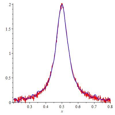
10                                                                            A. G. Khoee et al.

function of one parameter (x), so the Legendre series of it would be what we
have written above.
   By doing some manipulation, the Equation (16) can be written as:

                               ∂u ∂ 2 u                             ∂u ∂ 2 u

          ∆t                                   ∆t
 un+1 −            F n+1 (u, x, t,, 2 ) = un +      Fin+1 (u, x, t,   , 2) .
          2                    ∂x ∂x           2                    ∂x ∂x
                                                                             (18)
    To save the writing we name the left side of the above equation (18) as
Lun+1 (x) that is unknown and we should find it approximately later and the
left side of it as f n (x) which is defined.
    The following minimization problem must be solved in order to solve the
anisotropic diffusion equation by using the LS-SVR:

                                           1         1
                                     min     kwk2 + γ kek2
                                     w,e   2         2

                       s.t. Lun+1 (xi ) = f n (xi ) + ei , i = 1, . . . , n

   where xi are the training points that are selected over [0, 1]. We call the
above method, ”Collocation LS-SVR”.
   An alternative idea is to apply the orthogonality of the kernel to change
the minimization problem as it follows:

                                           1         1
                                     min     kwk2 + γ kek2
                                     w,e   2         2

               s.t. hLun+1 (x), φi (x)i = hf n (x), φi (x)i, i = 1, . . . , n

where
R      xi are the training points which is selected in Ω = [0, 1] and hf (x), g(x)i =
 Ω
   f (x)g(x)dx.  We call the above method, ”Galerkin LS-SVR”.
                                                            PN
Remark 1 The orthogonality of the kernel gives hu, ui = i=0 wi2 , so the en-
ergy of the signal in the objective function, computed by the weights, facilitates
the smoothing, i.e., the term kwk2 in minimization problem of Collocation LS-
SVR or Galerkin LS-SVR that is related to Thikonov regularization plays an
important role in signal smoothing.

Remark 2 The boundedness property (12) provides a control in error propa-
gation and the symmetric property (11) reduces the computational cost in the
method of LS-SVR.

     The training points may be chosen either by:
 • Selecting equidistance points or,
 • Selecting these point as the roots of Legendre polynomials.
A LS-SVR for anisotropic diffusion filtering 11
A good choice may be done by a meta-heuristic algorithm to take into
account the oscillations in the current state of the signal.
Both minimization problems of Collocation LS-SVR and Galerkin LS-SVR
can be reduced to a system of algebraic equations by using Lagrange multi-
pliers method [2] that is solved by a nonlinear solver such as the Newton
method. An alternative approach is to use nonlinear optimization methods
like line-search or trust-region algorithms.
We solve the anisotropic diffusion equation by using nonlinear LS-SVR
with Legendre polynomial function as its kernel (2.2) with particular boundary
conditions as its constraints, expressed as:
• un+1 (0) = un (0), (n = 0)
• un+1 (1) = un (1), (n = 0)
• u0 (x) = f (x), (input (noisy) signal)
By the evolution of a noisy signal in this process, it will lead to a smoothed
signal.
3.3 Overall algorithm
To sum up the proposed approach, the following algorithm is presented:
Algorithm 1: pseudo code
f (x) ←the initial signal;
u0 ← f (x);
du0 ← first derivative of u0 ;
ddu0 ← second derivative of u0 ;
c ← Perona-Malik coefficient (4) or (5);
∆t ← time step value (3.1);
for n ← 0 to M do
PN
un+1 ← i=0 wi φi (x) (17);
dun+1 ← first derivative of u1 ;
ddun+1 ← second derivative of u1 ;
for i ← 0 to N do
ei ← Lun+1 (xi ) − f n (xi ) 3.2;
end
Solving the specific minimization problem as described in the
Section 3.2;
end
4 Numerical results and discussion
In this section, two illustrative numerical examples will be provided to clarify
the efficiency of the proposed approach. First, we introduce the data gener-
ation method, which is used for our computational experiments. Next, these
examples are reported in the rest of the paper in detail.12 A. G. Khoee et al.
4.1 Data generation
Normally, we can simulate a noisy signal by adding white noise to the spectral
peak which can be defined as Gaussian peaks, Lorentzian peaks, and their
combinations.
Due to the fact that Pearson VII function is equivalent to another param-
eterization of the Student-t distribution function, it can generate the afore-
mentioned peaks as well [11] which is defined as below:
A
g(x) = (19)
x−µ 2 1
[1 + 4 σ 2q − 1 ]
where A, µ, and σ are related to the height, position, and width of the peak,
respectively. As a rule, when the parameter q is equal to 1, the function is a
Lorentzian peak. As the value of parameter q increases, the function converts
to the Gaussian peak.
As we mentioned above, we need to add white noise to these peaks to
generate the required data, which the white noise can be created by generating
random numbers in a particular range by ”GenerateGaussian” function in
Maple and using cubic spline to connect these points to get a continuous
function.
4.2 Numerical observations
Here, we reported the numerical results by implementing our approach using
Maple 2018 on a laptop with configuration: Intel(R) core(TM) i7-4720HQ CPU
@ 2.60 GHz and 12GB of RAM.
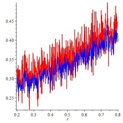
As a convention in all test cases, the red plot is the noisy signal and the
blue one is the smoothed signal.
For the first test case, we have used the data generation method we dis-
cussed in the previous section (4.1). With the particular parameters as ex-
pressed here:
1 1 1
A = 2, q= , σ= , µ= (20)
5 2 2
By the evolution of the first test case generated data as an input signal
in the algorithm 1 it will lead to smoothed signal as it is noticeable in the
following plots:A LS-SVR for anisotropic diffusion filtering 13 (a) After 0.1 seconds, SNR = 14.49373. (b) After 0.2 seconds, SNR = 16.68975. (c) After 0.3 seconds, SNR = 22.23075. (d) After 0.4 seconds, SNR = 26.67823. Fig. 1: Displaying the evolution of the first test case over [0.2, 0.8], the elapsed evolution time and calculated SNR are labeled below of each plot. As can be perceived from the SNR values of the first test case shown in Figure 1, the input signal has been smoothed well. Furthermore, to prove the strength of our presented approach, we have made a comparison between our proposed method and the Savitzky-Golay method here. We have done the Savitzky-Golay quadratic smoothing method with the filter width of 9; it can be noted that this size of filter width resembles more effective than other sizes, empirically.
14                                                             A. G. Khoee et al.

     For this purpose, the following plot and report are provided:

Fig. 2: Savitzky-Golay quadratic smoothing for the first test case with the
filter width of 9, SNR = -2.40262.

     As it is obvious, our proposed method has smoothed the noisy signal more
efficient than the Savitzky-Golay method without demolishing the peak, while
the Savitzky-Golay method has destroyed the peak without omitting all un-
wanted features well, according to the SNR values.
    Note that, since the classical signal smoothing methods, which are based
on moving average concept same like the Savitzky-Golay method, destroys
the beginning and the end of the signal, and because usually, the critical data
does not exist at the beginning and the end of a signal, we have reported the
information over [0.2, 0.8], in order to gain a fair comparison.
   For the second test case, we have done the same method as the first test
case in order to generate data by modifying some parameters, as stated here:

                   A = 2,      q = 2,     σ = 1.5,     µ=3                  (21)

    By the evolution of the second test case generated data as an input signal
in the algorithm 1 it will lead to smoothed signal as it is noticeable in the
following plots:
A LS-SVR for anisotropic diffusion filtering 15
(a) After 0.1 seconds, SNR = 29.58323. (b) After 0.2 seconds, SNR = 31.53024.
(c) After 0.3 seconds, SNR = 36.64582. (d) After 0.4 seconds, SNR = 40.18162.
Fig. 3: Displaying the evolution of the second test case over [0.2, 0.8], the
elapsed evolution time and calculated SNR are labeled below of each plot.
As can be perceived from the SNR values of the second test case shown in
Figure 3, the input signal has been smoothed well.
As in the first test case, we made a comparison with Savitzky-Golay method,
for the second test case, we have the following plot and report to address a
comparison with our proposed method.16 A. G. Khoee et al.
Fig. 4: Savitzky-Golay quadratic smoothing for the second test case with the
filter width of 9, SNR = 14.36374.
As reported from the SNR values show in the second test case, our pro-
posed method performs better than the Savitzky-Golay method in the signal
smoothing process.
According to numerical results, it is clear that the signal smoothing is done
successfully by the presented approach:
the 1st test case the 2nd test case
after 0.1 seconds 14.49373 29.58323
after 0.2 seconds 16.68975 31.53024
after 0.3 seconds 22.23075 36.64582
after 0.4 seconds 26.67823 40.18162
Table 1: The SNR values of test cases over time elapsed
Consequently, as time goes by, it becomes smoother as the SNR value
increases. In other words, higher SNR value in a test case means it has less
noise.
One of the advantages of this method is that we can smooth the signal as
far as we need by altering the hyperparameters. It is essential to mention that
the cease of the elapsed time of the input signal evolution to become smooth,
should be done by monitoring the SNR value.A LS-SVR for anisotropic diffusion filtering 17
5 conclusion
The proposed approach for signal smoothing based on anisotropic diffusion is
presented in a machine learning framework by using the LS-SVR with orthog-
onal kernel is proved to be highly competent for signal smoothing. In order to
optimize our method’s computational cost, we have used the Crank-Nicolson
method for discretization in time besides using orthogonal polynomials as the
LS-SVR kernel. It is clear that our approach is based on evolution in time; this
is important because, in this method, the smoothing rate can be controlled.
Numerical experiments confirm the validity and efficiency of our presented ap-
proach. It is seen that the method does not destroy edges rather preserving it.
We can consider it as a capable algorithm and could be used as an adaptive
signal smoothing method.
Conflict of interest
The authors declare that they have no conflict of interest.
References
1. Abdallah, M.B., Malek, J., Azar, A.T., Belmabrouk, H., Monreal, J.E., Krissian, K.:
Adaptive noise-reducing anisotropic diffusion filter. Neural Computing and Applications
27(5), 1273–1300 (2016)
2. Belytschko, T., Lu, Y.Y., Gu, L.: Element-free galerkin methods. International journal
for numerical methods in engineering 37(2), 229–256 (1994)
3. Bishop, C.M.: Pattern recognition and machine learning. springer (2006)
4. Byun, H., Lee, S.W.: Applications of support vector machines for pattern recognition: A
survey. In: International Workshop on Support Vector Machines, pp. 213–236. Springer
(2002)
5. Cristianini, N., Shawe-Taylor, J., et al.: An introduction to support vector machines
and other kernel-based learning methods. Cambridge university press (2000)
6. Delkhosh, M., Parand, K., Hadian-Rasanan, A.H.: A development of Lagrange interpo-
lation, part i: Theory. arXiv preprint arXiv:1904.12145 (2019)
7. Duda, R.O., Hart, P.E., Stork, D.G.: Pattern classification. John Wiley & Sons (2012)
8. Ganapathiraju, A., Hamaker, J., Picone, J.: Applications of support vector machines to
speech recognition. IEEE Transactions on Signal Processing 52(8), 2348–2355 (2004)
9. He, H., Ghodsi, A.: Rare class classification by support vector machine. In: 2010 20th
International Conference on Pattern Recognition, pp. 548–551. IEEE (2010)
10. Hieftje, G., Holder, B., Maddux, A., Lim, R.: Digital smoothing of electroanalytical
data based on the fourier transformation. Analytical Chemistry 45(2), 277–284 (1973)
11. Li, Y., Jiang, M.: Spatial-fractional order diffusion filtering. Journal of Mathematical
Chemistry 56(1), 257–267 (2018)
12. Li, Y., Liu, F., Turner, I.W., Li, T.: Time-fractional diffusion equation for signal smooth-
ing. Applied Mathematics and Computation 326, 108–116 (2018)
13. Lysaker, M., Lundervold, A., Tai, X.C.: Noise removal using fourth-order partial differ-
ential equation with applications to medical magnetic resonance images in space and
time. IEEE Transactions on Image Processing 12(12), 1579–1590 (2003)
14. Ma, J., Huang, W., Segarra, S., Ribeiro, A.: Diffusion filtering of graph signals and its
use in recommendation systems. In: 2016 IEEE International Conference on Acoustics,
Speech and Signal Processing, pp. 4563–4567. IEEE (2016)18 A. G. Khoee et al.
15. Mehrkanoon, S., Falck, T., Suykens, J.A.: Approximate solutions to ordinary differential
equations using least squares support vector machines. IEEE Transactions on Neural
Networks and Learning Systems 23(9), 1356–1367 (2012)
16. Mehrkanoon, S., Suykens, J.A.: Learning solutions to partial differential equations using
ls-svm. Neurocomputing 159, 105–116 (2015)
17. Meyer-Baese, A., Schmid, V.J.: Pattern recognition and signal analysis in medical imag-
ing. Elsevier (2014)
18. Osuna, E.E.: Support vector machines: Training and applications. Ph.D. thesis, Mas-
sachusetts Institute of Technology (1998)
19. Parand, K., Aghaei, A., Jani, M., Ghodsi, A.: A new approach to the numerical solution
of fredholm integral equations using least squares-support vector regression. Mathemat-
ics and Computers in Simulation 180, 114–128 (2021)
20. Parand, K., Nikarya, M.: A numerical method to solve the 1D and the 2D reaction
diffusion equation based on Bessel functions and Jacobian free Newton-Krylov subspace
methods. The European Physical Journal Plus 132(11), 496 (2017)
21. Perona, P., Malik, J.: Scale-space and edge detection using anisotropic diffusion. IEEE
Transactions on pattern analysis and machine intelligence 12(7), 629–639 (1990)
22. Raghavan, V.V., Gudivada, V.N., Govindaraju, V., Rao, C.R.: Cognitive computing:
Theory and applications. Elsevier (2016)
23. Schafer, R.W., et al.: What is a savitzky-golay filter. IEEE Signal Processing Magazine
28(4), 111–117 (2011)
24. Schölkopf, B., Tsuda, K., Vert, J.P.: Support vector machine applications in computa-
tional biology. MIT press (2004)
25. Shen, J., Tang, T., Wang, L.L.: Spectral methods: algorithms, analysis and applications,
vol. 41. Springer Science & Business Media (2011)
26. Suykens, J.A., Vandewalle, J.: Least squares support vector machine classifiers. Neural
processing letters 9(3), 293–300 (1999)
27. Tong, S., Koller, D.: Support vector machine active learning with applications to text
classification. Journal of machine learning research 2(Nov), 45–66 (2001)
28. Uçak K, G.G.: Online support vector regression based adaptive narma-l2 controller for
nonlinear systems. Neural Processing Letters 53(1), 405–428 (2021)
29. Vapnik, V.: The nature of statistical learning theory. Springer science & business media
(2013)
30. Wang, L.: Support vector machines: theory and applications, vol. 177. Springer Science
& Business Media (2005)
31. Witkin, A.P.: Scale-space filtering. In: Readings in Computer Vision, pp. 329–332.
Elsevier (1987)You can also read