Randomized Trees for Real-Time Keypoint Recognition
←
→
Page content transcription
If your browser does not render page correctly, please read the page content below
Randomized Trees for Real-Time Keypoint Recognition

                           Vincent Lepetit        Pascal Lagger       Pascal Fua
                                         Computer Vision Laboratory
             École Polytechnique Fédérale de Lausanne (EPFL) 1015 Lausanne, Switzerland
                       Email: {Vincent.Lepetit, Pascal.Lagger, Pascal.Fua}@epfl.ch

                        Abstract                                of views of individual keypoints. If the object can be as-
   In earlier work, we proposed treating wide baseline          sumed to be locally planar, this is done by simply warp-
matching of feature points as a classification problem, in      ing image patches around the points under affine or ho-
which each class corresponds to the set of all possible views   mographic deformations. Otherwise, given the 3D model,
of such a point. We used a K-mean plus Nearest Neighbor         we use standard Computer Graphics texture-mapping tech-
classifier to validate our approach, mostly because it was      niques. This second approach relaxes the planarity assump-
simple to implement. It has proved effective but still too      tions. At run-time, we can then use a powerful and fast
slow for real-time use.                                         classification technique to decide to which view set, if any,
   In this paper, we advocate instead the use of randomized     an observed feature belongs. This method is as effective
trees as the classification technique. It is both fast enough   and much faster than the usual way of computing local de-
for real-time performance and more robust. It also gives us     scriptors and comparing their responses. Once potential
a principled way not only to match keypoints but to select      correspondences have been established between the inter-
during a training phase those that are the most recogniz-       est points of the input image and those lying on the object,
able ones. This results in a real-time system able to detect    we apply a standard RANSAC-based method to estimate
and position in 3D planar, non-planar, and even deformable      the 3D pose.
objects. It is robust to illuminations changes, scale changes
and occlusions.                                                    In previous work [8], we used a K-mean plus Nearest
                                                                Neighbor classifier to validate our approach, mostly be-
                                                                cause it was simple to implement. It has proved effective
1. Introduction                                                 but still too slow for real-time use. Here, we advocate in-
Wide baseline keypoint matching has proved to be an effec-      stead the use of randomized trees [9] as the classification
tive tool for applications ranging from camera registration     technique. It is both faster and more robust, at the possi-
to object detection. Since the pioneering work by Schmid        ble expense of additional training time. Furthermore, it also
and Mohr [1], the algorithms have become ever more robust       gives us a principled way, not only to recognize keypoints,
to scale, viewpoint, illumination changes and partial occlu-    but also to select during the training phase those that yield
sions [2, 3, 4, 5, 6, 7].                                       the best recognition rate. As a result, even though we use
   These wide baseline matching methods, however, are           a monoscale algorithm for keypoint extraction [10], we can
typically designed to match two images but do not take ad-      achieve scale-invariance across a range of scales by using
vantage of the fact that, for object detection and pose esti-   training images at different resolutions and retaining only
mation purposes, both a 3D object model and several train-      those keypoints that are stable within the range.
ing images may be available. As shown in Figs 1 and 2,
our goal is to incorporate this additional information into        In short, the contribution of this paper is not only a faster
a keypoint recognizer that is both robust and fast enough       algorithm but also one that is more robust through the ap-
for real-time object detection, whether or not the object is    propriate selection of keypoints to be recognized.
planar.
   The key ingredient of our approach is to treat wide base-       In the remainder of the paper, we first discuss related
line matching of feature points as a classification problem,    work and recall how wide baseline matching can be stated
in which each class corresponds to the set of all possible      as a classification problem. We then present the proposed
views of such a point. During training, given at least one      keypoint selection method, detail our new classification
image of the target object, we synthesize a large number        method based on randomized trees, and comment the re-
                                                                sults.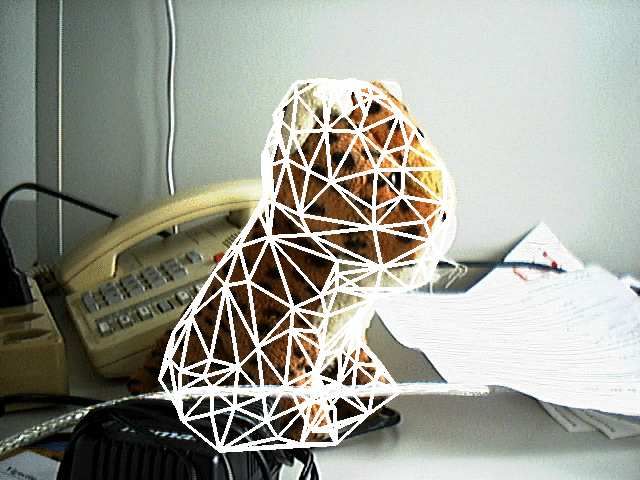
Figure 1. Detection of a book in a video sequence: The book is detected independently and suc-
cessfully in all subsequent frames at 25Hz in 640×480 images on a standard PC, in spite of partial
occlusion, cluttered background, motion blur, large illumination and pose changes. In the last two
frames, we add the inevitable virtual teapot to show we also recover 3D pose. A video sequence is
available at http://cvlab.epfl.ch/research/augm/detect.html
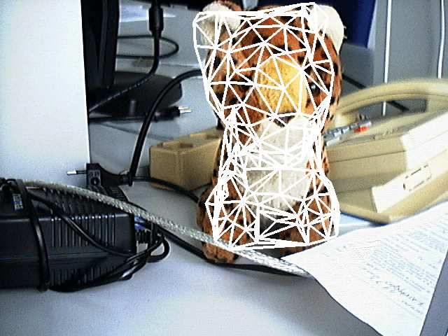
Figure 2. The method is just as effective for 3D objects. In this experiment, we detected the teddy
tiger using a 3D model reconstructed from several views such as the two first images on the left.
2. Related Work proaches to be effective, feature point extraction and char-
acterization should be insensitive to viewpoint and illumi-
In the area of automated 3D object detection, we can distin- nation changes. Scale-invariant feature extraction can be
guish between “Global” and “Local” approaches. achieved by using Harris detector [13] at several Gaussian
Global ones use statistical classification techniques to derivative scales, or by considering local optima of pyrami-
compare an input image to several training images of an dal difference-of-Gaussian filters in scale-space [7]. Miko-
object of interest and decide whether or not it appears in lajczyck et al. [4] have also defined an affine invariant point
this input image. The methods used range from relatively detector to handle larger viewpoint changes, that has been
simple methods such as Principal Component Analysis and used for 3D object recognition [14], but it relies on an iter-
Nearest Neighbor search [11] to more sophisticated ones ative estimation that would be too slow for our purposes.
such as AdaBoost and classifiers cascade to achieve real- Given the extracted feature points, various local descrip-
time detection of human faces at varying scales [12]. Such tors have been proposed: Schmid and Mohr [1] compute
approaches, however, are not particularly good at handling rotation invariant descriptors as functions of relatively high
occlusions, cluttered backgrounds, or the fact that the pose order image derivatives to achieve orientation invariance.
of the target object may be very different from those in the Baumberg [3] uses a variant of the Fourier-Mellin transfor-
training set. Furthermore, these global methods cannot pro- mation to achieve rotation invariance. He also gives an al-
vide accurate 3D pose estimation. gorithm to remove stretch and skew and obtain an affine
By contrast, local approaches use simple 2D features invariant characterization. Allezard et al. [15] represent
such as corners or edges, which makes them resistant to the keypoint neighborhood by a hierarchical sampling, and
partial occlusions and cluttered backgrounds: Even if some rotation invariance is obtained by starting the circular sam-
features are missing, the object can still be detected as pling with respect to the gradient direction. Tuytelaars and
long as enough are found and matched. Spurious matches al. [2] fit an ellipse to the texture around local intensity ex-
can be removed by enforcing geometric constraints, such trema to obtain correspondences remarkably robust to view-
as epipolar constraints between different views or full 3D point changes. Lowe [7] introduces a descriptor called SIFT
constraints if an object model is available. For local ap- based on several orientation histograms, that is not fully
2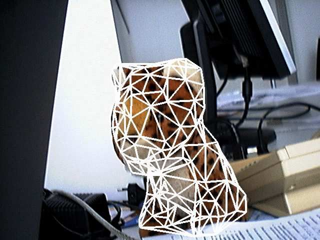
affine invariant but tolerates significant local deformations.
Most of these methods are too slow for real-time processing,
except for [5] that introduces Maximally Stable Extremal
Regions to achieve near frame rate matching of stable re-
gions. By contrast, our classification-based method runs
easily at frame rate, because it shifts much of the compu-
tational burden to a training phase and, as a result, reduces
the cost of online matching while increasing its robustness.
   Classification as a technique for wide baseline matching
has also been explored by [16] in parallel to our previous
work. In this approach, the training set is iteratively built
from incoming frames, and kernel PCA is used for classi-                   Figure 3. The most stable keypoints selected
fication. While this is interesting for applications when a                by our method on the book cover and the
training stage is not possible, our own method allows to de-               teddy tiger.
tect the object under unseen positions since we synthesize
new views. The classification method described in this pa-
per also has a lower complexity than their approach.

3. Keypoint Matching as Classification                                     Figure 4. An example of generated views for
                                                                           the book cover and the teddy tiger, and the
Let us first recall how matching keypoints found in an in-                 extracted keypoints for these views.
put image against keypoints on a target object O can be
naturally formulated as a classification problem [8]. Dur-
ing training, we construct a set K = {k1 . . . kN } of N
                                                                        4. Building the Training Set
prominent keypoints lying on the object. At runtime, given              In [8], we built the view sets by first extracting the keypoints
an input patch p(kinput ) centered at a keypoint kinput ex-             ki in the given original images then generating new views
tracted in the input image, we want to decide whether or                of each keypoint independently. As depicted in Fig.4, it is
not it can be an view of one of the N keypoints ki . In other           more effective to generate new views of the whole object,
words, we want to assign to p a class label Y (p) ∈ C =                 and extract keypoints in these views. This approach allows
{−1, 1, 2, . . . , N }, where the −1 label denotes all the points       us to solve in a simple way several fundamental problems
that do not belong to the object. Y cannot be directly ob-              at no additional computation cost at run-time: We can eas-
served and we aim at constructing a classifier Ŷ such as               ily determine stable keypoints under noise and perspective
P (Y 6= Ŷ ) is small.                                                  distortion, which helps making the matching robust to noise
   In other recognition tasks, such as face or character                and cluttered background.
recognition, large training sets of labeled data are usually
available. However, for automated pose estimation, it would             4.1. Local Planarity Assumptions
be impractical to require a very large number of sample im-             If the object can be assumed to be locally planar, a new
ages. Instead, to achieve robustness with respect to pose               view can be synthesized by warping a training image of the
and complex illumination changes, we use a small number                 object using an affine transformation that approximates the
of images and synthesize many new views of the object us-               actual homography. The affine transformations can be de-
ing simple rendering techniques to train our classifier: This           composed as: A = Rθ R−1     φ SRφ , where Rθ and Rφ are
approach gives us a virtually infinite training set to perform          two rotation matrices respectively parameterized by the an-
the classification.                                                     gles θ and φ, and S = diag [λ1 , λ2 ] is a scaling matrix. In
    For each keypoint, we can then constitute a sampling of             this paper, we use a random sampling of the affine trans-
its view set, that is the set of all its possible appearances           formations space, the angles θ and φ varying in the range
under different viewing conditions. This sampling allows                [−π; +π], and the scales λ1 and λ2 varying in the range
us to use statistical classification techniques to learn them           [0.2; 1.8]. Those ranges are much larger than the ones used
during an offline stage, and, finally, to perform the actual            in our earlier work, and can be handled because we now de-
classification at run-time. This gives us a set of matches              termine the most stable points and thanks to our new classi-
that lets us estimate the pose.                                         fication method.

                                                                    3
4.2. Relaxing the Planarity Assumptions
One advantage of our approach is that we can exploit the
knowledge of a 3D model if available. Such a model is
very useful to capture complex appearance changes due to
changes in the pose of a non convex 3D object, including
occlusions and non-affine warping. Given the 3D model,
we use standard Computer Graphics texture-mapping tech-
niques to generate new views under perspective transforma-
tions.
   In the case of the teddy tiger of Fig.2, we used Image
Modeler1 to reconstruct its 3D model. An automated recon-
struction method could also have been used, another alter-
native would have been to use image-based rendering tech-
                                                                                  Figure 5. First row: Patches centered at
niques to generate the new views.
                                                                                  a keypoint extracted in several new views,
                                                                                  synthesized using random affine transfor-
4.3. Keypoint Selection                                                           mations and white noise addition. Second
We are looking for a set of keypoints K = {ki } lying on                          row: Same patches after orientation correc-
the object to detect, and expressed in a reference system                         tion and Gaussian smoothing. These prepro-
related to this object. We should retain the keypoints with a                     cessed patches are used to train the keypoint
good probability P (k) to be extracted in the input views at                      classifier. Third and fourth rows: Same as be-
run-time.                                                                         fore for another keypoint located on the bor-
                                                                                  der of the book.
4.3.1. Finding Stable Keypoints
Let T denote the geometric transformation used to generate
a new view, and k e a keypoint extracted in this view. T is
an affine transformation, or a projection if the 3D model is
available. By applying T −1 to k,e we can recover its corre-
sponding keypoint k in the reference system. Thus, P (k)
can be estimated for keypoints lying on the objects from                          Figure 6. In the case of the teddy tiger, we
several generated views. The set K is then constructed by                         restricted the range of acceptable poses and
retaining keypoints ki with a high P (ki ). In our experi-                        the orientation correction was not used.
ments, we retain the 200 first keypoints according to this
measure. Fig. 3 shows the keypoints selected on the book                       generated views. To simulate a cluttered background, the
cover and the teddy tiger.                                                     new object view is rendered over a complex random back-
   The training set for keypoint ki is then built by collecting                ground. That way, the system is trained with images similar
the neighborhood p of the corresponding k   e in the generated                 to those at run-time.
images, as shown in Figs. 5 and 6.
                                                                               5. Keypoint Recognition
4.3.2. Robustness to Image Noise
                                                                               In [8], we used a K-mean plus Nearest Neighbor classifier
When a keypoint is detected in two different images, its pre-                  to validate our approach, because it is simple to implement
cise location may shift a bit due to image noise or viewpoint                  and it gives good results. Nevertheless, such classifier is
changes. In practice, such a positional shift results in large                 known to be one of the less efficient classification meth-
errors of direct cross-correlation measures. One solution is                   ods. We show in this section that randomized trees are bet-
to iteratively refine the point localization [4], which can be                 ter suited to our keypoint recognition problem, because they
costly.                                                                        allow very fast recognition and they naturally handle multi-
    In our method, this problem is directly handled by the                     class problems.
                                   e in the synthesized views:
fact that we extract the keypoints k
These images should be as close as possible to actual im-                      5.1. Randomized Trees
ages captured from a camera, and we add white noise to the
                                                                               Randomized trees are simple but powerful tools for clas-
   1 ImageModeler   is a commercial product fromRealviz(tm)  that allows       sification, introduced and applied to recognition of hand-
3D reconstruction from several views with manual intervention.                 written digits in [9]. [17] also applied them to recognition

                                                                           4
of 3–D objects. We quickly recall here the principles of                                            m
randomized trees for the unfamiliar reader. As depicted by
                                                                                          <                        >
Fig. 7, each non-terminal node of a tree contains a simple                                              ~
test that splits the image space. In our experiments, we use
tests of the type: “Is this pixel brighter than this one ?”.                      m                 m                  m

Each leaf contains an estimate based on training data of the
conditional distribution over the classes given that an image
reaches that leaf. A new image is classified by dropping it
down the tree, and, in the one tree case, attributing it the
class with the maximal conditional probability stored in the
leaf it reaches.
    We construct the trees in the classical, top-down man-
ner, where the tests are chosen by a greedy algorithm to                  Figure 7. Type of tree used for keypoint recog-
best separate the given examples, according to the expected               nition. The nodes contain tests comparing
gain of information. The process of selecting a test is re-               two pixels in the keypoint neighborhood; the
peated for each non-terminal descendant node, using only                  leaves contain the dl posterior distributions.
the training examples falling in that node. The recursion is
stopped when the node receives too few examples, or when               5.3. Node Tests
it reaches a given depth.                                              In practice, we use ternary tests based on the difference of
    Since the numbers of classes, training examples and pos-           intensities of two pixels taken in the neighborhood of the
sible tests are large in our case, building the optimal tree be-       keypoint:
comes quickly intractable. Instead we grow multiple, ran-                  If I(p, m1 ) − I(p, m2 )         < −τ   go to child 1;
domized trees: For each tree, we retain a small random sub-                If |I(p, m1 ) − I(p, m2 )|       ≤ +τ   go to child 2;
set of training examples and only a limited random sample                  If I(p, m1 ) − I(p, m2 )         > +τ   go to child 3.
of tests at each node, to obtain weak dependency between
the trees. More details about the trees construction can be            I(p, m) is the intensity of patch p after the preprocessing
found in [10].                                                         step described in Section 5.2, at pixel location m. m1 and
                                                                       m2 are two pixel locations chosen to optimize the expected
                                                                       gain of information as described above. τ is a threshold de-
5.2. Preprocessing                                                     ciding in which range two intensities should be considered
In order to make the classification task easier, the patches p         as similar. In the results presented in this paper, we take τ
                                                                       to be equal to 10.
of the training set or at run-time are preprocessed to remove
                                                                           This test is very simple and requires only pixel intensi-
some variations within the classes attributable to perspec-
tive and noise.                                                        ties comparisons. Nevertheless, because of the efficiency
                                                                       of randomized trees, it yields reliable classification results.
    The generated views are first smoothed using a Gaussian
                                                                       We tried other tests based on weighted sums of intensities
filter. We also use the method of [7] to attribute a 2D ori-
                                                                       a la Adaboost, on gradients or on Haar wavelets without
entation to the keypoints and achieve some normalization.
                                                                       significant improvements on the classification rate.
The orientation is estimated from the histogram of gradient
directions in a patch centered at the keypoint. Note that we           5.4. Run Time Keypoint Recognition
do not require a particularly stable method, since the same
method is used for training and run-time recognition. We               Once the randomized trees T1 , . . . , TL are built, the pos-
just want it to be reliable enough to reduce the variability           terior distributions P (Y = c|T = Tl , reached leaf = η)
within the same class. Once the orientation of an extracted            can be estimated for each terminal node η from the train-
keypoint is estimated, its neighborhood is rectified as shown          ing set. At runtime, the patches p centered at the keypoints
Fig. 5.                                                                extracted in the input image are preprocessed and dropped
                                                                       down the trees. Following [9], if dl (p) denotes the posterior
    Illumination changes are usually handled by normaliz-
                                                                       distribution in the node of tree Tl reached by a patch p, p is
ing the views intensities in some way, for example by nor-
                                                                       classified considering the average of the distributions dl (p):
malizing by the L2 norm of the intensities. We show be-
low that our randomized trees allow to skip this step. The                                                       1 X
                                                                             Ŷ (p) = argmax dc (p) = argmax               dl (p)
classification indeed relies on tests comparing intensities of                            c                 c    L
                                                                                                                   l=1...L
pixels. This avoids the use of an arbitrary normalization
                                                                           c
method and makes the classification very robust to illumi-                d (p) is the average of the posterior probabilities of class
nation changes.                                                        c and constitutes a good measure of the match confidence.

                                                                   5
100
                                                            inliers %age using tree depth = 5
                                                          inliers %age using tree depth = 10
                                                          inliers %age using tree depth = 15

                       80
   Inlier percentage

                       60

                                                                                                            Figure 9. Re-usability of the set of trees: A
                       40
                                                                                                            new object is presented to the system, and
                                                                                                            the posterior probabilities are updated. The
                       20                                                                                   new object can then be detected.

                        0
                             0      5      10        15             20               25         30
                                                Tree Number

   Figure 8. Percentage of correctly classified
   views with respect to the number of trees,
   using trees of depth 5, 10, and 15.

We can estimate during training a threshold Dc to decide if
the match is correct or not with a given confidence s:

                             P (Y (p) = c|Ŷ (p) = c, dc (p) > Dc ) > s

   In practice we take s = 90%. Keypoints giving dc (p)
lower than Dc are considered as keypoints detected on the
background, or misclassified keypoints, and are therefore                                                   Figure 10. Comparison with SIFT. When too
rejected. It leaves a small number of outlier matches, and                                                  much perspective distorts the object image,
the pose of the object is found by RANSAC after few itera-                                                  the SIFT approach gives only few matches
tions.                                                                                                      (left), while our approach is not perturbed
                                                                                                            (right).
5.5. Performance
The correct classification rate P (Ŷ (p) = c|Y (p) = c)
                                                                                                         lished in real-time. The estimated pose is then accurate and
of our classifier can then be measured using new random
                                                                                                         stable enough for Augmented Reality as shown Fig. 1.
views. The graph of Fig. 8 represents the percentage of
                                                                                                             We compared our results with those obtained using the
keypoints correctly classified, with respect to the number
                                                                                                         executable that implements the SIFT method [7] kindly pro-
of trees, for several maximal depths for the trees. The graph
                                                                                                         vided by David Lowe. As shown in Fig. 10, when too much
shows no real differences between taking trees of depth 10
                                                                                                         perspective distorts the object view, this method gives only
or 15, so we can use trees with limited depth. It also shows
                                                                                                         few matches, while ours is not perturbed. Ours is also much
that 20 trees are enough to reach a recognition rate of 80%.
                                                                                                         faster. For a fair comparison, remember that we take advan-
Growing 20 trees of depth 10 takes about 15 minutes on a
                                                                                                         tage of a training stage possible in object detection applica-
standard PC.
                                                                                                         tions, while the SIFT method can also be used to match two
    Since the classifier works by combining the responses
                                                                                                         given images. Another difference is that we cannot handle
of sub-optimal trees, we tried to re-use trees grown for a
first object for another object, as shown Fig. 9: We updated
the posterior probabilities in the terminal nodes, but kept
the same tests in the non-terminal nodes. We experienced
a slight drop of performance, but not enough to prevent the
system from recognizing the new object. In this case, the
time required for training drops to less than one minute.

6. Results
6.1. Planar Objects                                                                                         Figure 11. Detection of the book: Inlier
We first tried our algorithm on planar objects. Fig. 11 shows                                               matches established in real-time under sev-
matches between the training image and input images estab-                                                  eral poses.

                                                                                                     6
References
                                                                     [1] C. Schmid and R. Mohr, “Local Grayvalue Invariants for Image Re-
                                                                         trieval,” IEEE Transactions on Pattern Analysis and Machine Intel-
                                                                         ligence, vol. 19, no. 5, pp. 530–534, May 1997.
                                                                     [2] T. Tuytelaars and L. VanGool, “Wide Baseline Stereo Matching
                                                                         based on Local, Affinely Invariant Regions,” in British Machine Vi-
                                                                         sion Conference, 2000, pp. 412–422.
                                                                     [3] A. Baumberg, “Reliable Feature Matching across Widely Separated
   Figure 12. Deformable objects: the object is                          Views,” in Conference on Computer Vision and Pattern Recognition,
   detected and its deformation estimated, us-                           2000, pp. 774–781.
   ing the method described in [18].                                 [4] K. Mikolajczyk and C. Schmid, “An Affine Invariant Interest Point
                                                                         Detector,” in European Conference on Computer Vision. 2002, pp.
                                                                         128–142, Springer, Copenhagen.
as much scale changes as SIFT because we do not use (yet)            [5] J. Matas, O. Chum, U. Martin, and T. Pajdla, “Robust Wide Base-
a multi-scale keypoint detection.                                        line Stereo from Maximally Stable Extremal Regions,” in British
                                                                         Machine Vision Conference, London, UK, September 2002, pp. 384–
                                                                         393.
6.2. Detecting a 3D Object                                           [6] F. Schaffalitzky and A. Zisserman, “Multi-View Matching for Un-
                                                                         ordered Image Sets, or ”How Do I Organize My holiday Snaps?”,”
Fig. 2 shows results of the detection of a teddy tiger. As               in Proceedings of European Conference on Computer Vision, 2002,
mentioned above, its 3D textured model was reconstructed                 pp. 414–431.
from several views with the help of ImageModeler. It can             [7] D.G. Lowe, “Distinctive Image Features from Scale-Invariant Key-
                                                                         points,” International Journal of Computer Vision, vol. 20, no. 2, pp.
be detected from different sides, and front and up views.                91–110, 2004.
                                                                     [8] V. Lepetit, J. Pilet, and P. Fua, “Point Matching as a Classification
                                                                         Problem for Fast and Robust Object Pose Estimation,” in Conference
6.3. Detecting Deformable Objects                                        on Computer Vision and Pattern Recognition, Washington, DC, June
                                                                         2004.
Our method is also used in [18] to detect deformable objects
                                                                     [9] Y. Amit and D. Geman, “Shape Quantization and Recognition with
and estimate their deformation in real-time. The matches                 Randomized Trees,” Neural Computation, vol. 9, no. 7, pp. 1545–
are used not only to detect but also to compute a precise                1588, 1997.
mapping from a model image to the input image as shown              [10] V. Lepetit and P. Fua, “Towards Recognizing Feature Points using
Fig. 12.                                                                 Classification Trees ,” Technical Report IC/2004/74, EPFL, 2004.
                                                                    [11] S. K. Nayar, S. A. Nene, and H. Murase, “Real-Time 100 Object
                                                                         Recognition System,” IEEE Transactions on Pattern Analysis and
7. Conclusion and Perspectives                                           Machine Intelligence, vol. 18, no. 12, pp. 1186–1198, 1996.
                                                                    [12] P. Viola and M. Jones, “Rapid Object Detection using a Boosted
We proposed an approach to keypoint matching for object                  Cascade of Simple Features,” in Conference on Computer Vision
                                                                         and Pattern Recognition, 2001, pp. 511–518.
pose estimation based on classification. We showed that
                                                                    [13] C.G. Harris and M.J. Stephens, “A Combined Corner and Edge De-
using randomized trees yields a powerful matching method                 tector,” in Fourth Alvey Vision Conference, Manchester, 1988.
well adapted to object detection.                                   [14] F. Rothganger, S. Lazebnik, C. Schmid, and J. Ponce, “3D Object
   Our current approach to keypoint recognition relies on                Modeling and Recognition using Affine-Invariant Patches and Multi-
comparing pixel values in small neighborhoods around                     View Spatial Constraints,” in Conference on Computer Vision and
                                                                         Pattern Recognition, June 2003.
these keypoints. It works very well for textured objects,
                                                                    [15] N. Allezard, M. Dhome, and F. Jurie, “Recognition of 3D Textured
but loses its effectiveness in the absence of texture. To in-
                                                                         Objects by Mixing View-Based and Model-Based Representations,”
crease the range of applicability of our approach, we will               in International Conference on Pattern Recognition, Barcelona,
investigate the use of other additional image features, such             Spain, Sep 2000, pp. 960–963.
as spread gradient [19]. We believe our randomized tree ap-         [16] J. Meltzer, M.-H. Yang, R. Gupta, and S. Soatto, “Multiple View Fea-
proach to keypoint matching to be ideal to find out those                ture Descriptors from Image Sequences via Kernel Principal Com-
                                                                         ponent Analysis,” in Proceedings of European Conference on Com-
that are most informative in any given situation and, thus,              puter Vision, may 2004, pp. 215–227.
to allow us to mix different image features in a natural way.
                                                                    [17] B. Jedynak and F. Fleuret, “Reconnaissance d’objets 3D à l’aide
                                                                         d’arbres de classification,” in Proceedings of Image’Com, 1996.
                                                                    [18] J. Pilet, V. Lepetit, and P. Fua, “Real-Time Non-Rigid Surface Detec-
                                                                         tion,” in Conference on Computer Vision and Pattern Recognition,
Acknowledgements                                                         San Diego, CA, June 2005.
The authors would like to thank François Fleuret for sug-          [19] Y. Amit, D. Geman, and X. Fan, “A coarse-to-fine strategy for multi-
gesting to use randomized trees and for his insightful com-              class shape detection,” IEEE Transactions on Pattern Analysis and
                                                                         Machine Intelligence, 2004.
ments.

                                                                7


You can also read