A New BEM Modeling Algorithm for Size-Dependent Thermopiezoelectric Problems in Smart Nanostructures
←
→
Page content transcription
If your browser does not render page correctly, please read the page content below
Computers, Materials & Continua                                                             Tech Science Press
DOI:10.32604/cmc.2021.018191
Article

    A New BEM Modeling Algorithm for Size-Dependent Thermopiezoelectric
                   Problems in Smart Nanostructures
                                     Mohamed Abdelsabour Fahmy1,2, *

        1
         Department of Mathematics, Jamoum University College, Umm Al-Qura University, Alshohdaa, 25371,
                                            Jamoum, Makkah, Saudi Arabia
     2
       Department of Basic Sciences, Faculty of Computers and Informatics, Suez Canal University, New Campus,
                                                 Ismailia, 41522, Egypt
                *
                  Corresponding Author: Mohamed Abdelsabour Fahmy. Email: maselim@uqu.edu.sa
                                 Received: 28 February 2021; Accepted: 09 April 2021

                 Abstract: The main objective of this paper is to introduce a new theory
                 called size-dependent thermopiezoelectricity for smart nanostructures. The
                 proposed theory includes the combination of thermoelastic and piezoelectric
                 influences which enable us to describe the deformation and mechanical behav-
                 iors of smart nanostructures subjected to thermal, and piezoelectric loadings.
                 Because of difficulty of experimental research problems associated with the
                 proposed theory. Therefore, we propose a new boundary element method
                 (BEM) formulation and algorithm for the solution of such problems, which
                 involve temperatures, normal heat fluxes, displacements, couple-tractions,
                 rotations, force-tractions, electric displacement, and normal electric displace-
                 ment as primary variables within the BEM formulation. The computational
                 performance of the proposed methodology has been demonstrated by using
                 the generalized modified shift-splitting (GMSS) iteration method to solve
                 the linear systems resulting from the BEM discretization. GMSS advantages
                 are investigated and compared with other iterative methods. The numerical
                 results are depicted graphically to show the size-dependent effects of ther-
                 mopiezoelectricity, thermoelasticity, piezoelectricity, and elasticity theories
                 of nanostructures. The numerical results also show the effects of the size-
                 dependent and piezoelectric on the displacement components. The validity,
                 efficiency and accuracy of the proposed BEM formulation and algorithm
                 have been demonstrated. The findings of the current study contribute to the
                 further development of technological and industrial applications of smart
                 nanostructures.

                 Keywords: Boundary element method; size-dependent thermopiezoelectricity;
                 smart nanostructures

1 Introduction
    Nanoscience is that science through which atoms can be moved and manipulated in order to
obtain the properties we need in a specific field of life, as for nanotechnology, it is concerned with

                     This work is licensed under a Creative Commons Attribution 4.0 International License,
                     which permits unrestricted use, distribution, and reproduction in any medium, provided
                     the original work is properly cited.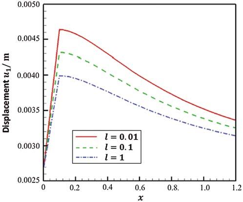
932                                                                          CMC, 2021, vol.69, no.1

manufacturing devices that can be used to study the properties of nanomaterials [1,2]. Nanostruc-
tures are one of the main products of nanotechnology. A nanostructure is a structure that has at
least one dimension equal or less than 100 nanometers. Understanding the mechanical behaviour
of deformed nanostructures is of great importance due to their applications in all fields such as
industry, medicine, renewable energy, military and civil and architecture Engineering. In the field
of industry, certain nanoparticles can be used in the manufacture of filters to purify and desalinate
water more efficiently than other types of filters, and they are also used as a heat insulator with
high efficiency. Some nanomaterials such as tungsten carbide and silicon carbide are distinguished
by their high strength compared to ordinary materials, so they are used in the manufacture of
some tools Cutting and drilling. Dust and water-repellent paints, clothing, and glass can also be
made [3]. Recent developments in nanoscale electronics and photonics might lead to new applica-
tions such as high-density memory, high-speed transistors and high-resolution lithography [4–6]. In
the medical field, certain nanoparticles can be used as drug-carrying materials, as these materials
have a special sensitivity to the place to which the drug is intended to be sent, so when they
reach it inside the human body, they release the drug accurately, in addition to promising research
confirming the possibility of using nanomaterials as a treatment for cancer. Gold nanoparticles are
also used in home testing devices to detect pregnancy. Nanowires are used as nanoscale biosensors
to detect a large number of diseases in their early stages [7,8]. In the field of renewable energy,
nanomaterials are involved in the manufacture of solar cells that are used in the production of
electrical energy, where materials such as cobalt oxide or semi-conductive materials in general
such as silicon and germanium are deposited on glass sheets or silica plates and because these
materials have a nanoscale size, the surface area that is exposed to sunlight is greater, and thus
we ensure that we absorb the largest amount of sunlight in a single cell. The panel usually
consists of hundreds of solar cells that are connected through an electrical circuit that converts
solar energy into electrical energy. In the military field, nanomaterials enter into the manufacture
of nanoscale cylinders that are characterized by strength and rigidity, in addition to a storage
capacity a million times greater than regular computers, the manufacture of military clothing
that has the ability to absorb radar waves in order to stealth and infiltrate, and the manufacture
of nanosatellites [9–11]. In the field of building and construction, some nanomaterials such as
titanium dioxide TiO2, carbon nanotubes CNTs and silica nanoparticles are added to concrete
to increase the durability and hardness of the concrete in addition to increasing its resistance to
water penetration. Size-dependent porothermoelastic [12–15] interactions play a significant role in
many areas of nanotechnology applications. Because of computational complexity in solving size-
dependent thermopiezoelectric problems not having any general analytical solution [16], therefore,
numerical methods should be developed to solve such problems. Among these numerical methods
is the boundary element method (BEM) that has been used for engineering models [17], bioheat
transfer models [18], and nanostructures [19]. The main feature of BEM [20] over the domain type
methods [21] is that only boundary of the considered domain needs to be discretized. This feature
is of great importance for solving complex nanoscience and nanotechnology problems with fewer
elements, and requires less computational cost, less preparation of input data, and therefore easier
to use.
     In the present paper, we introduce a new theory called size-dependent thermopiezoelectricity
for smart nanostructures to describe the mechanical behaviors of deformed nanostructures sub-
jected to various types of mechanical, thermal, and piezoelectric loadings. Also, we develop a new
boundary element formulation for solving the deformation problems associated with the proposed
theory. The numerical results illustrate the size-dependent effects on the thermo-piezoelectric,
thermoelastic, piezoelectric, and elastic smart nanostructures. The numerical results also show the
CMC, 2021, vol.69, no.1                                                                              933

effects of the length scale parameter and piezoelectric coefficient on the displacement components,
and confirm the validity, efficiency and accuracy of the proposed BEM formulation and algorithm.

2 Formulation of the Problem
     Consider a size-dependent thermopiezoelectric nanostructure occupies the cylindrical region
V (cross section of the nanostructure in the x1 x2 -plane) that bounded by S, such that x3-axis
parallel to the cylinder axis, as shown in Fig. 1. We take nα to be the outward unit vector that
is perpendicular to the boundary surface S as follows
           dxβ
nα = εαβ                                                                                              (1)
            ds
where εαβ (ε12 = −ε21 = 1, ε11 = ε22 = 0) is the two-dimensional permutation symbol.

                 Figure 1: Size-dependent thermopiezoelectric nanostructure definition

    In the two-dimensional plane, all quantities are independent of x3 . The deformation is
described by the displacement vector u = (u1 , u2 ), and the electric effect is specified by the electric
potential φ
    The rotation component is
            1              1
ω = ω3 =       u2, 1 − u1,2 = εαβ uβ, α                                                               (2)
            2                2
where
    The electric field components are
Eα = −φ, α                                                                                            (3)

    The strain tensor and the mean curvature vector
      1
eαβ = uα,β + uβ, α                                                                                    (4)
      2
               1
kα = εαβ k3β = εαβ ω, β                                                                               (5)
               2

where      kα k1 = k32 = 12 ω, 2 , k2 = −k31 = − 12 ω, 1   is the        mean      curvature      vector,

                   1
kαβ k3α = −kα3 = ω, α is the pseudo mean curvature tensor.
                   2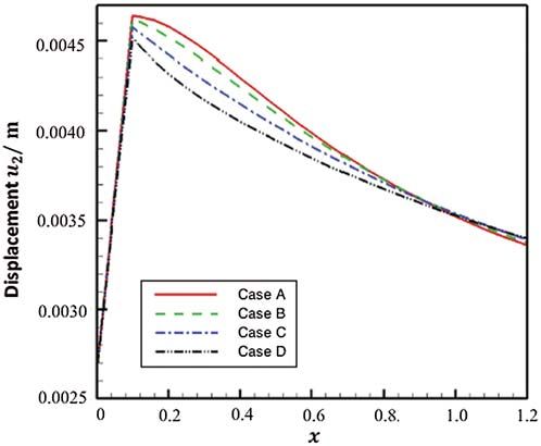
934                                                                           CMC, 2021, vol.69, no.1

   The true couple-stress vector Mi can be expressed in terms of pseudo couple-stress tensor
Mkj as
    1
Mi = εijk Mkj                                                                                      (6)
    2
where the true couple-stress vector Mi satisfies Mα = εαβ M3β , M1 = −M23 , M2 = M13 , M3 =
M21 = 0, and Mij = −Mji , and εijk is the three-dimensional Levi–Civita permutation symbol.
       The force-stress tensor can be decomposed into the following two parts
σαβ = σ(αβ) + σ[αβ]                                                                                (7)
where σαβ (σ3α = σα3 = 0) is the force-stress tensor, σ(αβ) is the symmetric force-stress tensor and
σ[αβ] is the skew-symmetric force-stress tensor.
   The electric field and mechanical deformation can induce polarization Pα in the piezoelectric
material. The electric displacement Dα is given as
Dα = ε0 Eα + Pα                                                                                    (8)
where ε0 is the vacuum permittivity, Eα is the electric field, Pα is the polarization of piezoelectric
material.
    The governing equations of size-dependent thermopiezoelectric problems in smart nanos-
tructures subjected to various types of mechanical, thermal and piezoelectric loadings can be
expressed as
       The entropy balance equation
−qα, α + Q = 0                                                                                     (9)
where qα is the heat flux vector.
       The force equilibrium equation
σβα, β + Fα = 0                                                                                   (10)
where Fα is the body force vector.
       The moment equilibrium equation
σ[βα] = −M[α, β] ,         σ[21] = −σ[12] = −M[1,2]                                               (11)

       The Gauss’s law for electric field can be expressed as
Dα, α = ρE                                                                                        (12)
where ρE is the volume electric charge density.
       Substitution of Eqs. (12) and (17) into force equilibrium Eq. (16) leads to

    σ(βα) − M[α, β]   ,β
                           + Fα = 0                                                               (13)

    The constitutive relations of size-dependent thermopiezoelectric nanostructures can be writ-
ten as:
       The heat flux vector equation
qα = −kT, α                                                                                       (14)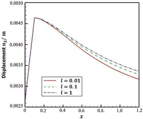
CMC, 2021, vol.69, no.1                                                                       935

     The symmetric force-stress equation
σ(αβ) = λeγ γ δαβ + 2μeαβ − (3λ + 2μ) αTδαβ                                                   (15)
where α is the coefficient of thermal expansion, δαβ is the Kronecker delta function
     the couple-stress equation
Mα = −8μl 2 kα + 2fEα                                                                         (16)
the electric displacement equation
Dα = εEα + 4fkα                                                                               (17)

    Also, the force-traction vector tα , couple-traction m, and normal electric displacement d can
be written as follows
tα = σβα nβ                                                                                   (18)
m = εβα Mα nβ = M2 n1 − M1 n2                                                                 (19)
d = Dα nα                                                                                     (20)
where f is the piezoelectric coefficient.
     The Lamé elastic constants λ ad μ for an isotropic material, can be related to the Poisson
ratio v and Young’s modulus E as
                              v
E = 2μ (1 + v) ,   λ = 2μ                                                                     (21)
                            1 − 2v
where v is the Poisson ratio, E is the Young’s modulus,
     The electric permittivity of the material can be defined as
ε = εr ε0                                                                                     (22)
where εr is relative permittivity.
     The material length scale parameter used in couple stress theories can be written as
     η
l2 =                                                                                          (23)
     μ
where η is the couple-stress parameter.
     Now, the total force-stress tensor σβα can be expressed as
                                                E
σβα = λeγ γ δαβ + 2μeαβ + 2μl 2 εαβ ∇ 2 ω −          αTδαβ                                    (24)
                                              1 − 2ν
     Hence, the governing Eqs. (9), (10) and (12) can be written as
k∇ 2 T + Q = 0                                                                                (25)
where k is the thermal conductivity, T is the temperature and Q is an external heat source.
                                                 E
 λ + μ 1 + l 2 ∇ 2 uβ, βα + μ 1 − l 2 ∇ 2 ∇ 2 uα −        αT, α + Fα = 0                    (26)
                                                   1 − 2ν
ε∇ 2 φ + ρE = 0                                                                               (27)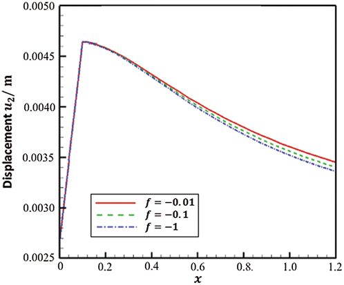
936                                                                                                          CMC, 2021, vol.69, no.1

    Now, the normal heat flux q, force-traction vector tα , couple-traction m, and normal electric
displacement d can be written as follows
              ∂T
q = qα nα = −k                                                                                                                  (28)
               ∂n

                                                                       E
tα = σβα nβ = λeγ γ δαβ + 2μeαβ + 2μl 2 εαβ ∇ 2 ω −                         αTδαβ nβ                                            (29)
                                                                     1 − 2ν
                   ∂ω       ∂φ
m = εβα μα nβ = 4μl 2  − 2f                                                                                                     (30)
                    ∂n      ∂s
               ∂φ      ∂ω
d = Dα nα = −ε    + 2f                                                                                                          (31)
               ∂n      ∂s

3 Boundary Conditions
     The considered boundary conditions may specify either temperature change T or normal heat
flux q
T=T       on ST                                                                                                                 (32)
q=q       on Sq ,    ST ∪ Sq = S,        ST ∩ Sq = ∅                                                                            (33)

      Displacements uα or force-tractions tα
uα = uα     on Su                                                                                                               (34)
tα = tα    on St ,       Su ∪ St = S,     Su ∩ St = ∅                                                                           (35)

      Rotation ω or couple-traction m
ω=ω       on Sω                                                                                                                 (36)
m=m        on Sm ,       Sω ∪ Sm = S,       Sω ∩ Sm = ∅                                                                         (37)
and electric potential φ or normal electric displacement d
φ=φ       on Sφ                                                                                                                 (38)

d = d on Sd ,        Sφ ∪ Sd = S,       Sφ ∩ Sd = ∅                                                                             (39)
where ST , Sq , Su , St , Sω , Sm , Sφ and Sd are the boundary parts at which the boundary values for
the temperature change T, the normal heat flux q, the displacement vector uα , the force-traction
vector tα , the rotation ω, the couple-traction m, the electric potential φ and the normal electric
displacement d are specified.

4 Boundary Element Implementation
    Now, we can write the boundary integral equations for temperature, displacements, rotation,
and potential as follows
  ∗                        ∗                                         ∗                                   ∗
cQ (ξ ) T (ξ ) −         qQ (x, ξ ) T (x) dS (x) = −            T Q (x, ξ ) q (x) dS (x) +           T Q (x, ξ ) Q (x) dV (x)   (40)
                     S                                      S                                    V
                           ∗                                     ∗                                   ∗
cαβ (ξ ) uα (ξ ) +       tFαβ (x, ξ ) uα (x) dS (x) +       mFβ (x, ξ ) ω (x) dS (x) +           hFβ (x, ξ ) T (x) dS (x)
                     S                                  S                                    S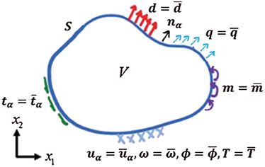
CMC, 2021, vol.69, no.1                                                                                                                    937

                 ∗                                        ∗                                         ∗
   +        dβF (x, ξ ) φ (x) dS (x) =               uFαβ (x, ξ ) tα (x) dS (x) +              ωβF (x, ξ ) m (x) dS (x)
       S                                         S                                         S
                 ∗                                    ∗                                        ∗
   +        uFαβ (x, ξ ) Fα (x) dV +             fβF (x, ξ ) q (x) dS (x) −                fβF (x, ξ ) Q (x) dV                            (41)
       V                                     S                                         V
                              ∗                                            ∗                                       ∗
cω (ξ ) ω (ξ ) +         tC
                          α (x, ξ ) uα (x) dS (x) +                   mC (x, ξ ) ω (x) dS (x) +                 d C (x, ξ ) φ (x) dS (x)
                     S                                            S                                         S
                 ∗                                            ∗                                         ∗
   =        uC
             α (x, ξ ) tα (x) dS (x) +               ωC (x, ξ ) m (x) dS (x) +                     uC
                                                                                                    α (x, ξ ) Fα (x) dV                    (42)
        S                                        S                                          V
                                  ∗                                        ∗
cφ (ξ ) φ (ξ ) +         mR (x, ξ ) ω (x) dS (x) +                    d R (x, ξ ) φ (x) dS (x)
                     S                                            S
                 ∗                                        ∗
   =        φ R (x, ξ ) d (x) dS (x) −               φ R (x, ξ ) ρE (x) dV                                                                 (43)
        S                                        V

where the superscripts Q∗ , F ∗ , C ∗ and R∗ are chosen to be kernel functions associated with
point heat source, point force, point couple and point electrical source infinite space fundamen-
tal solutions, respectively, and denotes the Cauchy principal value symbol. denotes the Cauchy
principal value symbol. The full details for the derivations of the fundamental solutions used in
the current formulation are given in [22–24].
    The integral Eqs. (40)–(43) in absence of body forces and volume charge density can be
written in matrix form as follows
⎡ ∗              ⎤    ⎡ Q∗                                          ⎤⎡       ⎤
 cQ (ξ ) T (ξ )         −q     0            0           0              T (x)
⎢                ⎥    ⎢ ∗                                           ⎥⎢       ⎥
⎢cαβ (ξ ) uα (ξ )⎥    ⎢hF      tFαβ (x, ξ ) mFβ (x, ξ ) dβF (x, ξ ) ⎥
                                  ∗            ∗           ∗
                                                                       uα (x)⎥
⎢                ⎥    ⎢ β                                           ⎥⎢⎢      ⎥ dS (x)
⎢ ω              ⎥+ ⎢                                               ⎥⎢       ⎥
⎢c (ξ ) ω (ξ ) ⎥    S ⎢0
                                   ∗            ∗           ∗
                               tα (x, ξ ) m (x, ξ ) d (x, ξ )⎦ ⎣
                                 C            C           C         ⎥  ω (x) ⎦
⎣                ⎦    ⎣
                                                                           ∗            ∗
  cφ (ξ ) φ (ξ )          0                   0                       mR (x, ξ )     d R (x, ξ )   φ (x)
         ⎡ Q∗                                                                      ⎤⎡        ⎤
           −ϑ         0                          0                     0               q (x)
         ⎢ ∗                                                                       ⎥⎢
         ⎢f F (x, ξ ) uF ∗ (x, ξ )                   F∗
                                                 ωβ (x, ξ )            0           ⎥ ⎢tα (x)⎥⎥
         ⎢β             αβ                                                         ⎥⎢        ⎥ dS (x)
   = ⎢                                                                             ⎥⎢                                                      (44)
         ⎢               ∗                           C∗                            ⎥ ⎣m (x) ⎥
       s 0
         ⎣            uCα (x, ξ )                ω        (x, ξ ) 0                ⎦         ⎦
                                                                               ∗
             0                        0          0                     φ R (x, ξ )     d (x)

     Now, it is convenient to rewrite Eq. (44) in compact index-notation form as

cIJ (ξ ) uI (ξ ) +           t∗IJ (x, ξ ) uI (x) dS (x) =             u∗IJ (x, ξ ) tI (x) dS (x)                                           (45)
                         S                                        s

where the generalized displacements uI in (45) include temperature T, displacement uα , rotation
ω and electric potential φ, respectively. Similarly, the generalized tractions tI include normal flux
q, force-tractions tα , couple-traction m and normal electric displacement d, respectively.
     This leads to the following linear algebraic equations system
Tu = Ut                                                                                                                                    (46)
938 CMC, 2021, vol.69, no.1
where T and U are dense matrices related with the left and right hand sides of Eq. (44),
respectively, and u represents the nodal boundary temperature, displacement, rotation and elec-
tric potential, respectively, while, t represents the nodal boundary normal flux, force-tractions,
couple-tractions and normal electric displacement, respectively.
which can be written as
AX = B (47)
where A is the non-symmetric dense matrix, B is the known boundary values vector and X is the
unknown boundary vector of unknown boundary values vector.
5 Numerical Results and Discussion
To illustrate the numerical calculations computed by the proposed methodology, we consider
the thermopiezoelectric nanoplate with free boundary conditions on the sides, as shown in Fig. 2.
A variable temperature field in the x2 -direction is generated by applying Tb and Tt to the bottom
and top surfaces, respectively. Also, a uniform electric field in the x2 -direction is generated by
applying constant electric potentials φb and φt to the bottom and top surfaces, respectively. Under
thermal and piezoelectric loadings, the plate deforms and becomes electrically polarized. As a
result, the thermal effect is specified by the thermal expansion coefficient α, the size dependent
effect is specified by one characteristic length scale parameter l, and the piezoelectric effect is
specified by one piezoelectric coefficient f .
Figure 2: Geometry of the free piezo-thermo-elastic nanoplate
The solid line represents the Case A that corresponds to the size-dependent thermo-
piezoelectric plates (α = 1, f = −1) . The dashed line represents the Case B which corresponds
to size-dependent thermoelastic plates (α = 1, f = 0). The dash-dot line represents the Case C
that corresponds to size-dependent piezoelectric plates (α = 0, f = −1). The dash-two dot line
represents the Case D which corresponds to size-dependent elastic plates (α = 0, f = 0).
Figs. 3 and 4 show the variation of the displacements u1 and u2 along x-axis for different
size-dependent theories. It can be seen from these figures that the differences between size-
dependent thermopiezoelectricity, size-dependent thermoelasticity, size-dependent piezoelectricity,
and size-dependent elasticity theories are very pronounced.
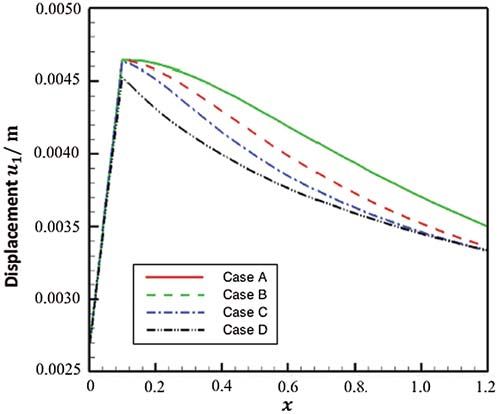
Figs. 5 and 6 show the variation of the displacements u1 and u2 along x-axis for different
values of length scale parameter l. It can be seen from these figures that the displacement u1
decreases with the increase of the length scale parameter l, while, the displacement u2 increases
with the increase of the length scale parameter l.CMC, 2021, vol.69, no.1 939
Figure 3: Variation of the displacement u1 along x-axis for different size-dependent theories
Figure 4: Variation of the displacement u2 along x-axis for different size-dependent theories
Figs. 7 and 8 show the variation of the displacements u1 and u2 along x-axis for different
values of piezoelectric coefficient f . It can be seen from these figures that the displacements u1
and u2 increase with the increase of piezoelectric coefficient f .
The efficiency of our proposed methodology has been demonstrated through the use of the
GMSS iteration method [25], which reduces the memory requirements and Processing time [26,27].
During our treatment of the considered problem, we implemented symmetric successive over relax-
ation (SSOR) [28], and preconditioned generalized shift-splitting (PGSS) iteration methods [29]
to solve the linear systems resulting from the BEM discretization. Tab. 1 illustrates the iterations
number (Iter.), processor time (CPU time), relative residual (Rr), and error (Err.) of the considered940 CMC, 2021, vol.69, no.1
methods computed for various length scale parameter values (l = 0.01, 0.1 and 1.0). It is shown
from Tab. 1 that the GMSS needs the lowest IT and CPU times, which implies that GMSS
method has better performance than SSOR and PGSS.
Figure 5: Variation of the displacement u1 along x-axis for different values of length scale
parameter l
Figure 6: Variation of the displacement u2 along x-axis for different values of length scale
parameter l
Tab. 2 summarizes the resulting numerical solutions for horizontal displacements u1 at points
A and B for different values of length scale parameter l (l = 0.01, 0.1 and 1.0). This table also
includes the finite element method (FEM) results of Sladek et al. [30], as well as the analyticalCMC, 2021, vol.69, no.1 941 solution of Yu et al. [31], it can be shown from Tab. 2 that the BEM results are in very good agreement with the FDM and analytical results. Thus, the validity and accuracy of the proposed BEM have been demonstrated. Figure 7: Variation of the displacement u1 along x-axis for different values of piezoelectric coefficient f Figure 8: Variation of the displacement u2 along x-axis for different values of piezoelectric coefficient f
942                                                                                CMC, 2021, vol.69, no.1

                       Table 1: Numerical results for the tested iteration methods
l                   Method            Iter.            CPU time              Rr                 Err.
0.01                GMSS              20               0.0115                1.94e−07           1.46e−09
                    SSOR              50               0.0559                5.47e−07           1.69e−07
                    PGSS              60               0.0725                6.99e−07           2.48e−06
0.1                 GMSS              30               0.0534                0.17e−06           2.03e−08
                    SSOR              80               0.2235                1.69e−05           4.49e−06
                    PGSS              100              0.3759                1.13e−04           0.55e−05
1.0                 GMSS              50               0.1754                2.19e−05           1.78e−07
                    SSOR              250              0.7936                1.78e−04           3.59e−05
                    PGSS              270              0.8947                1.19e−03           4.56e−04

              Table 2: Numerical values for horizontal displacement at points A and B
l          BEM                                FEM                              Analytical
           (u1 )A            (u1 )B           (u1 )A            (u1 )B         (u1 )A         (u1 )B
0.01       1.67878122        0.17597343       1.67878017        0.17597329     1.67878120     0.17597340
0.1        0.27564102        0.01015923       0.27564089        0.01015898     0.27564099     0.01015919
1.0        0.04096853        0.00281463       0.04096849        0.00281456     0.04096851     0.00281462

6 Conclusion
     —A new theory called size-dependent thermopiezoelectricity for smart nanostructures is
introduced.
    —Because of the benefits of the BEM such as dealing with more complicated shapes of
nanostructures and not requiring the discretization of the internal domain, also, it has low CPU
time and memory. Therefore, it is versatile and efficient method for modeling of size-dependent
thermopiezoelectric problems in smart nanostructures.
    —A new BEM formulation is developed for solving the problems associated with the proposed
theory, which involves temperatures, normal heat fluxes, displacements, couple-tractions, rotations,
force-tractions, electric displacement, and normal electric displacement as primary variables within
the BEM formulation.
    —The BEM is accelerated by using the GMSS, which reduces the total CPU time and number
of iterations.
    —The proposed theory includes the combination of thermoelastic and piezoelectric influences
which enable us to explain the differences between size-dependent thermopiezoelectricity, size-
dependent thermoelasticity, size-dependent piezoelectricity and size-dependent elasticity theories of
nanostructures.
    —Numerical findings are presented graphically to show the effects of the size-dependent and
piezoelectric on the displacement components.
       —The computational performance of the proposed methodology has been demonstrated.
CMC, 2021, vol.69, no.1 943
—The validity and accuracy of the proposed BEM technique have been demonstrated.
—From the proposed model that has been carried out using BEM formulation, it is possible
to conclude that our proposed technique is more convenient, cost-effective, highly accurate, and
has superiority over FDM or FEM.
—The proposed technique can be applied to study a wide variety of size-dependent problems
in smart nanostructures subjected to mechanical, thermal and piezoelectric loadings.
—It can be concluded that our study has a wide variety of applications in numerous
fields, such as electronics, chemistry, physics, biology, material science, optics, photonics, industry,
military, and even medicine.
—Current numerical results for the proposed theory and its related problems, may pro-
vide interesting information for nanophysicists, nanochemists, nanobiologists, nanotechnology
engineers, and nanoscience mathematicians as well as for computer scientists specializing in
nanotechnology.
Funding Statement: The author received no specific funding for this study.
Conflicts of Interest: The author declares that he has no conflicts of interest to report regarding
the present study.
References
[1] J. Ghanbari and R. Naghdabadi, “Multiscale nonlinear constitutive modeling of carbon nanostructures
based on interatomic potentials,” Computers, Materials & Continua, vol. 10, no. 1, pp. 41–64, 2009.
[2] A. Chakrabarty and T. Çağin, “Computational studies on mechanical and thermal properties of carbon
nanotube based nanostructures,” Computers, Materials & Continua, vol. 7, no. 3, pp. 167–190, 2008.
[3] S. N. Cha, J. S. Seo, S. M. Kim, H. J. Kim, Y. J. Park et al., “Sound-driven piezoelectric nanowire-based
nanogenerators,” Advanced Materials, vol. 22, no. 42, pp. 4726–4730, 2010.
[4] I. Voiculescu and A. N. Nordin, “Acoustic wave based MEMS devices for biosensing applications,”
Biosensors and Bioelectronics, vol. 33, no. 1, pp. 1–9, 2012.
[5] D. Shin, Y. Urzhumov, Y. Jung, G. Kang, S. Baek et al., “Broadband electromagnetic cloaking with
smart metamaterials,” Nature Communications, vol. 3, no. 11, pp. 1213, 2012.
[6] S. Zhang, B. Gu, H. Zhang, X. Q. Feng, R. Pan et al., “Propagation of love waves with surface effects
in an electrically-shorted piezoelectric nano film on a half-space elastic substrate,” Ultrasonics, vol. 66,
no. 3, pp. 65–71, 2016.
[7] I. F. Akyildiz and J. M. Jornet, “Electromagnetic wireless nanosensor networks,” Nano Communication
Networks, vol. 1, no. 1, pp. 3–19, 2010.
[8] J. He, X. Qi, Y. Miao, H. L. Wu, N. He et al., “Application of smart nanostructures in medicine,”
Nanomedicine, vol. 5, no. 7, pp. 1129–1138, 2010.
[9] A. Y. Al-Hossain, F. A. Farhoud and M. Ibrahim, “The mathematical model of reflection and refrac-
tion of plane quasi-vertical transverse waves at interface nanocomposite smart material,” Journal of
Computational and Theoretical Nanoscience, vol. 8, no. 7, pp. 1193–1202, 2011.
[10] L. L. Zhu and X. J. Zheng, “Stress field effects on phonon properties in spatially confined semicon-
ductor nanostructures,” Computers, Materials & Continua, vol. 18, no. 3, pp. 301–320, 2010.
[11] Y. Danlee, I. Huynen and C. Bailly, “Thin smart multilayer microwave absorber based on hybrid
structure of polymer and carbon nanotubes,” Applied Physics Letters, vol. 100, no. 21, pp. 213105, 2012.
[12] M. A. Ezzat, “State space approach to unsteady two-dimensional free convection flow through a porous
medium,” Canadian Journal of Physics, vol. 72, no. 5–6, pp. 311–317, 1994.944 CMC, 2021, vol.69, no.1
[13] M. Ezzat, M. Zakaria, O. Shaker and F. Barakat, “State space formulation to viscoelastic fluid flow of
magnetohydrodynamic free convection through a porous medium,” Acta Mechanica, vol. 119, no. 1–4,
pp. 147–164, 1996.
[14] M. A. Ezzat, “Free convection effects on perfectly conducting fluid,” International Journal of Engineering
Science, vol. 39, no. 7, pp. 799–819, 2001.
[15] M. A. Ezzat, “State space approach to solids and fluids,” Canadian Journal of Physics, vol. 86, no. 11,
pp. 1241–1250, 2008.
[16] A. R. Hadjesfandiari, “Size-dependent piezoelectricity,” International Journal of Solids and Structures,
vol. 50, no. 18, pp. 2781–2791, 2013.
[17] M. A. Fahmy, “Boundary element algorithm for nonlinear modeling and simulation of three tem-
perature anisotropic generalized micropolar piezothermoelasticity with memory-dependent derivative,”
International Journal of Applied Mechanics, vol. 12, no. 3, pp. 2050027, 2020.
[18] M. A. Fahmy, “A new boundary element algorithm for modeling and simulation of nonlinear thermal
stresses in micropolar FGA composites with temperature-dependent properties,” Advanced Modeling and
Simulation in Engineering Sciences, vol. 8, no. 6, pp. 1–23, 2021.
[19] M. A. Fahmy, “A new boundary element formulation for modeling and simulation of three-temperature
distributions in carbon nanotube fiber-reinforced composites with inclusions,” Mathematical Methods in
the Applied Science, (In Press), 2021.
[20] M. A. Fahmy, “A new boundary element algorithm for a general solution of nonlinear space-time
fractional dual-phase-lag bio-heat transfer problems during electromagnetic radiation,” Case Studies in
Thermal Engineering, vol. 25, no. 100918, pp. 1–11, 2021.
[21] B. T. Darrall, A. R. Hadjesfandiari and G. F. Dargush, “Size-dependent piezoelectricity: A 2D finite
element formulation for electric field-mean curvature coupling in dielectrics,” European Journal of
Mechanics-A/Solids, vol. 49, no. 1–2, pp. 308–320, 2015.
[22] A. R. Hadjesfandiari and G. F. Dargush, “Fundamental solutions for isotropic size-dependent couple
stress elasticity,” International Journal of Solids and Structures, vol. 50, no. 9, pp. 1253–1265, 2013.
[23] A. Hajesfandiari, A. R. Hadjesfandiari and G. F. Dargush, “Boundary element formulation for plane
problems in size-dependent piezoelectricity,” International Journal for Numerical Methods in Engineering,
vol. 108, no. 7, pp. 667–694, 2016.
[24] A. Hajesfandiari, A. R. Hadjesfandiari and G. F. Dargush, “Boundary element formulation for steady
state plane problems in size-dependent thermoelasticity,” Engineering Analysis with Boundary Elements,
vol. 82, no. 9, pp. 210–226, 2017.
[25] Z. G. Huang, L. G. Wang, Z. Xu and J. J. Cui, “The generalized modified shift-splitting preconditioners
for nonsymmetric saddle point problems,” Applied Mathematics and Computation, vol. 299, no. 4, pp. 95–
118, 2017.
[26] M. A. Fahmy, “A new BEM for fractional nonlinear generalized porothermoelastic wave propagation
problems,” Computers, Materials & Continua, vol. 68, no. 1, pp. 59–76, 2021.
[27] M. A. Fahmy, “A novel BEM for modeling and simulation of 3T nonlinear generalized anisotropic
micropolar-thermoelasticity theory with memory dependent derivative,” Computer Modeling in Engineer-
ing & Sciences, vol. 126, no. 1, pp. 175–199, 2021.
[28] T. S. Siahkolaei and D. K. Salkuyeh, “A preconditioned SSOR iteration method for solving complex
symmetric system of linear equations,” American Institute of Mathematical Sciences, vol. 9, no. 4,
pp. 483–492, 2019.
[29] Y. Xiao, Q. Wu and Y. Zhang, “Newton-PGSS and its improvement method for solving nonlinear
systems with saddle point Jacobian matrices,” Journal of Mathematics, vol. 2021, no. 636943, pp. 1–
18, 2021.
[30] J. Sladek, V. Sladek, M. Repka and C. L. Tan, “Size dependent thermo-piezoelectricity for in-plane
cracks,” Key Engineering Materials, vol. 827, no. 1, pp. 147–152, 2019.
[31] Y. J. Yu, X. G. Tian and X. R. Liu, “Size-dependent generalized thermoelasticity using Eringen’s
nonlocal model,” European Journal of Mechanics A/Solids, vol. 51, no. 5–6, pp. 96–106, 2015.You can also read