A new statistical graph model to systematically study associations between multivariate exposome data and multivariate metabolomics data - ISGlobal

A new statistical graph model to systematically
study associations between multivariate exposome
    data and multivariate metabolomics data

                       Qiong Wu

  Co-authors: Drs. Shuo Chen, Charles Ma, Donald Milton

                       April, 2021

   Q. Wu               ISGlobal (2021)          April, 2021   1 / 19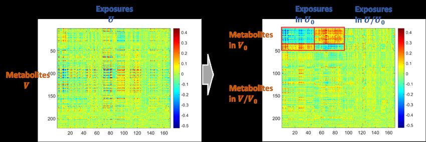

Outline

1   Introduction

2   Methods

3   Data Results

4   Summary

5   Github Files

         Q. Wu     ISGlobal (2021)   April, 2021   2 / 19

Introduction

   Association studies in multi-omics data
       Discover the systematic association patterns between a set(s) of
       multivariate correlated exposure variables and a set(s) of
       multivariate metabolomics (or gene/protein expression data);
       Study human responses to a mixture of environmental exposures:
       Multivariate predictors and multivariate outcomes.

      Q. Wu                  ISGlobal (2021)               April, 2021    3 / 19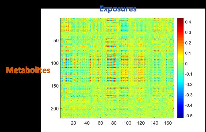

Goal

   Goal : parsimonious multivariate-multivariate association pattern
   detection, to select a set(s) of exposures and a set(s) of accordingly
   affected outcomes.
   Challenges:
        Univariate methods (a bag of pairwise associations)
        - false positive and negative associations can disrupt revealing the
        underlying systematic association patterns;
        Dimension reduction methods (e.g., principal component analysis or
        canonical correlation analysis)
        - limited to identify specific exposome and metabolome variables in
        the correlated components;
        Biclustering algorithms
        - miss the patterns by equally assigning variables to clusters.

       Q. Wu                   ISGlobal (2021)               April, 2021   4 / 19

Graph model setup

   We characterize the relationship as a Bipartite Graph
   G = (U, V, E, W ).
   Nodes U : all exposures; nodes V : all metabolites; and weighted
   edges W the marginal association measures (|U | × |V |).
   We focus on the subgraph G[U0 , V0 ], U0 ⊂ U and V0 ⊂ V of
   significant exposures-metabolites associations concentrated.

   Figure 1: A demonstration of the bipartite graph with subgraph G[U0 , V0 ].
   The right subfigure indicates G[U0 , V0 ] in G with nodes reordered.

       Q. Wu                      ISGlobal (2021)                  April, 2021   5 / 19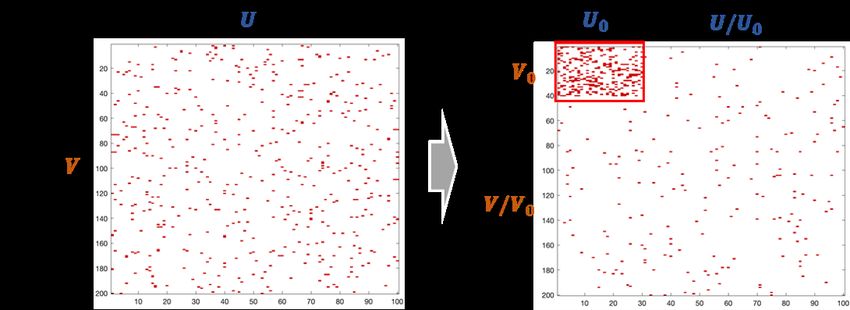

Association Patterns

   Figure 2: A demonstration of the bipartite graph with subgraph G[U0 , V0 ].
   The right subfigure indicates G[U0 , V0 ] in G with nodes reordered.

       Q. Wu                      ISGlobal (2021)                  April, 2021   6 / 19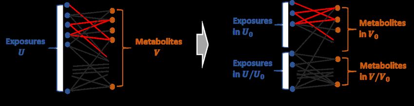

A false positive association edge is likely, but not
the systematic pattern
    Based on graph combinatorics, the probability that a non-trivial
    set of exposures are highly correlated with a non-trivial set of
    metabolitics converges to Zero under the null.

Lemma (Under null hypothesis/random graph)
Suppose G is observed from a random bipartite graph G(m, n, π).
G[Sγ , Tγ ] is a γ-quasi biclique with γ ∈ (π, 1). Let
m0 , n0 = Ω(max{m , n }) for some 0 <  < 1. Then for sufficiently
large m, n with c(π, γ)m0 ≥ 8 log n and c(π, γ)n0 ≥ 8 log m, we have
                                                              
                                                    1
        P (|Sγ | ≥ m0 , |Tγ | ≥ n0 ) ≤ 2mn · exp − c(γ, π)m0 n0 ,
                                                    4
                  n                         o−1
                        1             1
where c(a, b) =       (a−b)2
                               +   3(a−b)         .

        Q. Wu                           ISGlobal (2021)   April, 2021   7 / 19

Search for the systematic pattern by a generalized
density metric

   To detect a subgraph maximized edge density and subgraph size,
   we propose a generalized density metric:

                                        |W [S, T ]|
                         dλ (S, T ) =               ,                   (1)
                                         (|S||T |)λ

   with λ ∈ (0, 1).
   We output the subgraph as:

                      (S̃λ , T̃λ ) = arg max dλ (S, T )
                                        S,T

      Q. Wu                  ISGlobal (2021)              April, 2021   8 / 19

Likelihood-based method for λ estimation
   The likelihood of the bipartite graph with dense subgraph has
   form:
                                           aij
                                Y
                                                        1−aij
         L(π1 , π0 ; S, T, A) =   i∈S,j∈T π1 (1 − π1 )
                                                  a
                                        Y
                                ×                π0 ij (1 − π0 )1−aij ,
                                        i∈U/S or j∈V /T

   Therefore,
                      λ̂ = arg max Lλ (π1 , π0 ; S̃λ , T̃λ , A).
                               λ
   For weighted adjacency matrix, we binarize as
   Aij = {W (r)}ij = I(Wij > r).
   Consider the threshold r has a support {r1 , ...., rm } and
   corresponding probability {g(r1 ), ..., g(rm )}, we integrate r out:
                                      Z                             
       Lλ (π1 , π0 ; S̃λ , T̃λ , W ) = Lλ π1 , π0 ; S̃λ , T̃λ , W (r) g(r)dr.

       Q. Wu                       ISGlobal (2021)                 April, 2021   9 / 19

Greedy algorithm with given λ
Algorithm 1 Greedy algorithm with given λ
 1: procedure Algorithm
 2:      for c ∈ {c1 , c2 , ..., cL } do
 3:           S1 ← U , T1 ← V
 4:           for k=1 to n + m − 1 do
 5:                 let i ∈ Sk with: i = arg mini0 ∈Sk degX (i0 ; Sk , Tk );
 6:                 let j ∈ Tk with: j = arg minj 0 ∈Tk degY (j 0 ; Sk , Tk );
                        √
 7:                 if c degX (i; Sk , Tk ) ≤ √1c degY (j; Sk , Tk ) then
 8:                      Sk+1 ← Sk /{i} and Tk+1 ← Tk ;
 9:                 else
10:                      Sk+1 ← Sk and Tk+1 ← Tk /{j};
11:                 end if
12:           end for
13:           Output G[S c , T c ] that maximizes the density metric among
      G[S1 , T1 ], ..., G[Sn+m−1 , Tn+m1 ];
14:      end for
15:      Output G[S c∗ , T c∗ ] with largest density G[S c1 , T c1 ], ..., G[S cL , T cL ];
16:   end procedure
           Q. Wu                       ISGlobal (2021)                   April, 2021   10 / 19

Data results
   169 numeric exposure variables and 221 metabolites variables for
   1192 subjects;
   We observe the association matrix as pairwise correlation
   coefficients, although other metrics can be used (e.g., -log(p)
   values of regression coefficients).

     Figure 3: Association matrix between exposome and metabolites

       Q. Wu                  ISGlobal (2021)            April, 2021   11 / 19

Data results

   Figure 4: Detecting the systematic association patterns between multiple
   exposure variables and metabolomics

      Q. Wu                   ISGlobal (2021)              April, 2021   12 / 19

Data results

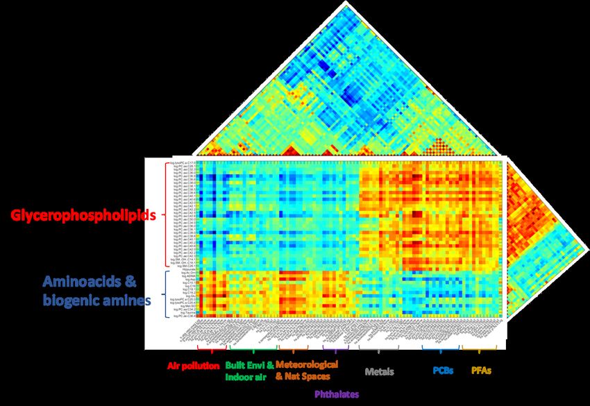
   Figure 5: Zoomed association patterns between multiple exposure
   variables and metabolomics
      Q. Wu                   ISGlobal (2021)             April, 2021   13 / 19

Data results

   Figure 6: Zoomed association patterns between multiple exposure
   variables and metabolomics

      Q. Wu                   ISGlobal (2021)             April, 2021   14 / 19

Selected metabolites can better explained by our
selected exposomes than all exposomes
   Full models:
                                     X
                    yv ∼ Xv βv =           xuv βuv ,   ∀v ∈ T̃λ̂
                                     u∈U

   where U represents the set of all exposures, T̃λ̂ is the set of
   metabolites within the detected subgraph.
   Reduced models:
                                   X
                yv ∼ Xvsub βvsub =     xuv βuv , ∀v ∈ T̃λ̂
                                      u∈S̃λ̂

   where S̃λ̂ is the set of exposures selected in the subgraph.
                               Number of predictors       R2
              Full models      169                        0.317 (0.080)
              Reduced models   92                         0.261 (0.085)

      Q. Wu                    ISGlobal (2021)                     April, 2021   15 / 19

Cross-validation performance

       Evaluate the performance using cross-validation (5-folds):
         - 80% data are used to fit the model (estimates β̂train );
         - 20% are testing data to predict ŷtest = Xtest β̂train
         - Predictive R2 , RMSE and MAE are calculated based on ŷtest and
           ytest
                              Predictive R2     RMSE   1
                                                                MAE   2

             Full models      0.116 (0.028)     0.373 (0.015)   0.295 (0.012)
             Reduced models   0.146 (0.033)     0.356 (0.013)   0.281 (0.010)

  1
      RMSE: Root Mean Squared Error
  2
      MAE: Mean Absolute Error
          Q. Wu                   ISGlobal (2021)                  April, 2021   16 / 19

Summary

  Identify systematic associations between multivariate exposome
  and multivariate metabolome variables, which can be generalized
  to other multi-omics data;
  Parsimonious multivariate-multivariate association pattern
  extraction via detecting subgraphs in a bipartite graph with
  concentrated association pairs via a computationally efficient
  algorithm;
  Distinguish systematic negative and positive association blocks;
  Exposures within the detected subgraph can explain the
  population variance of selected metabolites comparing to the
  whole set of exposures.

     Q. Wu                  ISGlobal (2021)            April, 2021   17 / 19

Github Files

   Matlab functions:
     - greedy bipar.m (maximize the density metric)
     - greedy lik fun.m (select the tunning parameter via likelihood)
     - NICE.m (refine the association pattern)
   Data analysis:
     -    prepare data.R
     -    code.m
     -    Output figures.m
     -    compare models.R
   Data results:
     -    meta merge.mat
     -    expos merge.mat
     -    expos meta res.mat
     -    Output figures.html (with a full list of variable names)

         Q. Wu                   ISGlobal (2021)               April, 2021   18 / 19

Thank you for your attention!

Q. Wu             ISGlobal (2021)       April, 2021   19 / 19