A Rotation Scheme for Accurately Computing Meteoroid Flux - SIAM
←
→
Page content transcription
If your browser does not render page correctly, please read the page content below
A Rotation Scheme for Accurately Computing
                                                     Meteoroid Flux

                                                                                             Anita Thomas1
                                                                                 Advisors: Martin Ratliff2 and Shuwang Li3

                          Abstract. Accurately estimating meteoroid flux helps analyze the risk of collisions while
                      spacecraft move in interplanetary space. Currently, NASA uses the Meteoroid Engineering
                      Model (MEM) to estimate meteoroid flux and the Bumper-ii code to evaluate damage to a
                      spacecraft structure. To help the Bumper algorithm evaluate potential damage, we develop
                      a rotation scheme that converts meteoroid flux information from the reference frame used
                      in the Meteoroid Engineering Model to Bumper’s reference frame as a spacecraft rotates in
                      space. Using randomly generated data, we show our average accuracy can be at least 98.6%.

                                 Key words. Meteoroid flux, quaternion rotation, solid angle bins.

                      1             Introduction
                      On February 15, 2013, a meteor explosion in Russia threatened many lives. The meteor
                      fractured 12 to 15 miles above Earth’s surface [7]. Broken windows sent shards of glass
                      flying through the air, thus injuring about 1200 people and causing $30 million in damages.
                      Because the object was coming from the general direction of the sun, telescopes were unable
                      to detect it in the sun’s glare [6]. Videos and news coverage of the distressing event under-
                      score the importance of continued research into meteoroid detection and risk analysis.

                      While the Russian meteor is a rare example of the threat posed by meteoroids, spacecraft
                      flying through interplanetary space frequently experience more commonplace collisions with
                      particle-sized meteoroids. Here we report on research that helps analyze that meteoroid risk.
                      Currently, NASA uses its Meteoroid Engineering Model (MEM) to estimate meteoroid flux
                      at a given point in space and the NASA Bumper-ii algorithm to evaluate potential dam-
                      age to a spacecraft structure. Output from MEM is fed into Bumper as input. Because
                      MEM is coded according to a reference frame derived from the spacecraft trajectory and
                      Bumper uses a reference frame fixed to the body of the spacecraft, this process only pro-
                      duces accurate results when the spacecraft maintains a constant orientation [1, 3]. In this
                      paper we develop an algorithm that rotates meteoroid flux information from MEM’s refer-
                      ence frame to Bumper’s reference frame as a spacecraft rotates in interplanetary space. This
                             1
                               Department of Applied Mathematics, Illinois Institute of Technology, Chicago. thomas1894@gmail.com
                             2
                               Reliability Engineering Office, NASA Jet Propulsion Laboratory, Caltech, J.M.Ratliff@jpl.nasa.gov
                             3
                               Department of Applied Mathematics, Illinois Institute of Technology, Chicago. sli@math.iit.edu

Copyright © SIAM
Unauthorized reproduction of this article is prohibited.This Contribution was produced by a member (or members) of the Jet Propulsion Laboratory, California Institute of
Technology, and is considered a work-for-hire. In accordance with the contract between the California Institute of Technology and the National Aeronautics and Space
Administration, the United States Government, and others acting on its behalf, shall have, for Governmental purposes, a royalty-free, nonexclusive, irrevocable, worldwide              263
license to publish, distribute, copy, exhibit and perform the work, in whole or in part, to authorize others to do so, to reproduce the final published and/or electronic form of the
Contribution, to include the work on the NASA/JPL Technical Reports Server web site, and to prepare derivative works including, but not limited to, abstracts, lectures, lecture
notes, press releases, reviews, textbooks, reprint books, and translations .
algorithm tracks the change in flux to a given area of the spacecraft, as the spacecraft rotates.
The idea is to visualize a sphere divided into solid-angle bins surrounding a spacecraft. The
use of a sphere represents the possibility of a meteoroid collision with a spacecraft from any
direction [1]. Each solid-angle bin is assigned its respective meteoroid flux (in pseudo-units
of particles per m2 per second per bin solid angle) [3]. When a spacecraft rotates, the bins
in MEM’s sphere no longer align with the bins in Bumper’s sphere. To recalculate the flux
in the spacecraft bins, we start by using MEM output to define spacecraft bins in spherical
coordinates (θ, φ, r). We fill each bin with dots and apportion a fraction of the bin flux to
each dot. A rotation then moves the dots to new bins. The fluxes of the new set of dots in
each spacecraft bin are summed to determine the new total flux in each bin.
This paper is organized as follows. In section 2, we describe the computing scheme. In
section 3, we show examples on accuracy measurement. In section 4, we give concluding
remarks and discuss future work.
2 Description of the Scheme
2.1 Quaternion Rotation Matrix
We use quaternion formalism to determine the dots’ new locations after a rotation. An in-
troduction to quaternions can be found in Kuipers [5]. Quaternions rotate coordinate frames
in 3-D using rotation information stored in a 4-D vector. The use of quaternions avoids at
least some of the singularities and modulus ambiguities that appear in the more commonly
used Euler angle representation of a rotation [9].
Quaternions consist of four elements: q1 , q2 , q3 and q4 . Although they provide no clear visual
representation, these four quaternion components together represent a rotation around some
axis through some angle of rotation. The quaternion vector that represents a spacecraft
rotation about the vector e is defined as
q1 e1 s
q2 e2 s
q = = , (1)
q3 e3 s
q4 c
where e is the axis of rotation, s is the value of sin( 2θ ), c is the value of cos( 2θ ), and θ is equal
to the angle of rotation [9]. The axes of rotation, in this case, correspond to the x, y, and
z axes. Note that in cases where the axis of rotation is not one of the coordinate axes, find
the eigenvector with eigenvalue equal to zero; by definition this eigenvector lies on the vector
264that remains the same before and after rotation (axis of rotation) [9].
Each rotation about the x, y, and z axes is represented by its own quaternion vector: qx , qy ,
and qz , respectively. These quaternion vectors can be used to find one rotation matrix that
represents a collective rotation about the x, y, and z axes. To do so, we first calculate the
quaternions representing a collective rotation around the x and y axes
q40 q30 −q20 q10
−q30 q40 q10 q20
qxyRot = q , (2)
q20 −q10 q40 q30 x
−q10 −q20 −q30 q40
where qx is the quaternion rotation vector representing a rotation around the x-axis and
q10 , q20 , q30 , q40 represent the quaternion components of qy [9].
We then calculate the quaternions corresponding to a collective rotation around the x, y,
and z axes, respectively,
q400 q300 −q200 q100
−q300 q400 q100 q200
qxyzRot = q , (3)
q200 −q100 q400 q300 xyRot
−q100 −q200 −q300 q400
where q100 , q200 , q300 , q400 represent the quaternion components of qz [9].
When used in this direction cosine matrix
q12 − q22 − q32 − q42 2(q1 q2 + q3 q4 ) 2(q1 q3 − q2 q4 )
A = 2(q1 q2 − q3 q4 ) −q12 + q22 − q32 + q42 2(q2 q3 + q1 q4 ) , (4)
2(q1 q3 + q2 q4 ) 2(q2 q3 − q1 q4 ) −q12 − q22 + q32 + q42
the quaternion components of qxyzRot form a 3 × 3 rotation matrix equal to its corresponding
Euler rotation matrix [9].
2652.2 Defining Spacecraft Bins
In this section, we provide an explanation of MEM’s outputs and discuss how that output is
reformatted for use in our rotation scheme. Figure 2.1 shows the top half of the solid angle
bin pattern corresponding to MEM output [1].
Figure 2.1: MEM output: solid angle bin pattern
In Figure 2.1, the angle φ refers to the elevation of a spacecraft bin and ranges from − π2 to
π
2
. The angle θ shows how far around the sphere a bin is located and ranges from zero to
2π [1].
Table 2.1 is a subset of MEM output.
A B C D E F G
1 1 1 -90 -85 0 120
2 1 2 -90 -85 120 240
3 1 3 -90 -85 240 360
4 2 1 -85 -80 0 40
5 2 2 -85 -80 40 80
6 2 3 -85 -80 80 120
7 2 4 -85 -80 120 160
8 2 5 -85 -80 160 200
9 2 6 -85 -80 200 240
10 2 7 -85 -80 240 280
11 2 8 -85 -80 280 320
12 2 9 -85 -80 320 360
Table 2.1: MEM output (subset)
266Column A defines a numbering scheme for the bins. Column B dentoes the row that a bin
lies in, and the column C indicates a bin’s location within its respective row. Columns D,
E, F, G of the MEM output represent the start and end φ and θ of every spacecraft bin. In
order to define the MEM angles in terms of standard spherical coordinates, the algorithm
employs the following procedure:
1. Change all angles from degrees to radians.
2. Switch the columns MEM calls θ and φ so that θ represents elevation and φ represents
the azimuth angle.
3. Flip the θ start and θ end vectors top to bottom to define bin one at the top of the
sphere.
4. Interchange the θ start and θ end vectors.
5. Subtract all angles in the θ start and θ end vectors from π2 , so that θ ranges from 0 to
π.
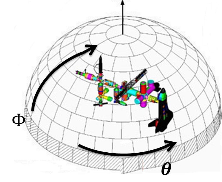
As an example, Figure 2.2 shows an arbitrary bin after the above modifications have been
implemented and Table 2.2 shows the θ and φ bounds of the twelve bins at the “top” of the
sphere after the above modifications have been implemented.
Figure 2.2: MEM output: solid angle bin example
267θstart θend φstart φend
0 0.0873 0 2.0944
0 0.0873 2.0944 4.1888
0 0.0873 4.1888 6.2832
0.0873 0.1745 0 0.6981
0.0873 0.1745 0.6981 1.3963
0.0873 0.1745 1.3963 2.0944
0.0873 0.1745 2.0944 2.7925
0.0873 0.1745 2.7925 3.4907
0.0873 0.1745 3.4907 4.1888
0.0873 0.1745 4.1888 4.8869
0.0873 0.1745 4.8869 5.5851
0.0873 0.1745 5.5851 6.2832
Table 2.2: MEM output modification: subset of bin θ and φ bounds
2.3 Defining Dots on Sphere
In this section, we explain one successful and three less successful means of defining dots
on the sphere. The successful method is described below and is immediately followed by
descriptions of the three less successful attempts.
When a spacecraft rotates, the bins on the MEM and Bumper spheres become unaligned.
To recalculate the flux in the spacecraft bins after rotation, the fraction of each MEM bin
that rotates into a spacecraft bin is determined and the corresponding flux in each of those
fractions is summed to define the new total flux in that spacecraft bin. In order to find the
fraction of each MEM bin that rotates into a spacecraft bin, each bin is filled with dots and
the fraction of dots that rotate into different spacecraft bins reveal the fraction of each MEM
bin that rotates into a spacecraft bin.
Each bin has an associated meteoroid flux (in pseudo-units of particles per m2 per second
per bin solid angle) [3]. Each dot in a bin represents a fraction of that flux. Since each dot
in a bin is assigned the same fraction of total flux per bin, it is important to distribute the
dots so that they also represent the same fraction of surface area within a bin. Because the
surface area of a bin varies with θ, more dots are assigned to areas of a bin with θ values
closer to the equator. To accomplish this skewed distribution, the algorithm divides each
bin into ten levels, as shown in Figure 2.3.
268Figure 2.3: Bin shapes
The triangle represents the bins at the poles and the trapezoid represents all other bins. Note
that bins on the bottom of the sphere are inverted. We will refer to the total number of dots
per bin and the total surface area per bin as N and S, respectively. We will refer to the total
number of dots per level and the total surface area per level as n and s, respectively. The
surface area in steradians of each level, s, within each bin is calculated and then multiplied by
the number of dots per steradian–calculated by dividing a user-defined value for the number
of dots per bin, N , by the surface area of each bin, S. The resulting number, rounded to
the nearest whole number, represents the number of randomly generated dots per level, n,
in each bin, or more compactly
(s)(N )
n= . (5)
S
This approach creates a fairly constant spatial distribution of dots within a bin, which results
in an even distribution of flux across the bin when each dot is assigned the same flux per
dot within the bin. Flux per dot is determined by dividing the flux per bin by the number
of dots in the bin.
Before implementing the distribution described above, we tested three other distributions.
The corresponding accuracies are summarized and explained in section 3 of this paper. These
distributions include
• Constant Step Size
Using a constant step size, we defined each dots’ θ coordinate from 0 to π and φ
coordinate from 0 to 2π. Each row of dots has an equal number of dots and each
column has an equal number of dots.
• Uniform Distribution
The agorithm generates uniformly distributed random numbers between 0 and π for θ
and between 0 and 2π for φ.
We attributed the less than acceptable accuracy of the above two distributions to the in-
creasing surface area of a sphere as θ nears the equator. As a result, we sought to implement
a distribution that accounts for this change in surface area by placing an increasing number
of dots in the bins as they neared the equator; this idea led to a Chebyshev distribution.
269• Chebyshev Nodes
Chebyshev polynomials of the first kind contain roots, or nodes, that interpolate poly-
nomials in the interval [−1, 1]. In this case, −1 represents the bottom of the sphere and
1 represents the top of the sphere. Chebyshev distributes points more heavily at the
poles, which is the opposite of what we needed. To adjust, we created two intervals,
shifted them π2 up and down, and used half of each interval [4]. We refer to the total
number of dots on the sphere as M .
The formulas we used to determine the θ part of the coordinates are
2k + 1
xk = cos π , (6)
2n + 2
π π
θk = (xk + 1) ± , (7)
2 2
where k = 1, 2, .., M [4].
To determine the corresponding φ part of the coordinates, we subtracted θk − θk−1 and
assigned that value as the step size for φ. So, φk ranges from 0 to 2π with stepsize
θk − θk−1 .
In total, we tested four distributions. The first three distributions refer to the first three we
coded–the less successful distributions. The fourth distribution refers to the final, successful
distribution.
2.4 Rotating Dots
In this section, we present the formulas used to rotate the dots on the sphere. To rotate the
dots through any angle about any axis, the dots’ coordinates are first changed from spherical
to Cartesian and then multiplied by a rotation matrix. The rotated Cartesian coordinates
are then transferred back into spherical coordinates.
The formulas
x = r sin(θ) cos(φ), (8)
y = r sin(θ) sin(φ), (9)
z = r cos(θ), (10)
change the dots from spherical to Cartesian points where r = 1 on a unit sphere [8].
270The formula
2
q1 − q22 − q32 − q42 2(q1 q2 + q3 q4 ) 2(q1 q3 − q2 q4 ) xi
qR = 2(q1 q2 − q3 q4 ) −q12 + q22 − q32 + q42 2(q2 q3 + q1 q4 ) yi , (11)
2(q1 q3 + q2 q4 ) 2(q2 q3 − q1 q4 ) −q12 − q22 + q32 + q42 zi
where q1 , q2 , q3 , and q4 are the quanternion components of qxyzRot and xi , yi , and zi are the
Cartesian components of each dot, rotates all the dots [9].
To convert the rotated dots from Cartesian to spherical, use the following formulas
z
θ = cos−1 , (12)
r
y
φ = tan−1 , (13)
x
with r = 1 [8].
Because the range of arctan spans π2 to − π2 , the algorithm checks the x and y components of
each rotated dot to determine which quadrant φ was supposed to end up in. If x is negative
and y is positive, π is added to φ. If x is negative and y is negative, π is also added to φ.
Finally, if x is positive and y is negative, 2π is added to φ.
2.5 Calculating New Flux
To identify the bin each dot rotates into, the spherical coordinates of each dot are compared
to the start and end spherical coordinates of each bin. The fluxes of the dots in each bin are
summed to determine the new flux in each spacecraft bin. The flux is then flipped from top
to bottom to adhere to the bin numbering system used by Bumper. The overall algorithm
is in Algorithm 1.
271Algorithm 1 Numerical algorithm
Input: rotation angles (x, y, and z axes)
1: Compute quaternion rotation matrix
2: Load/Read in MEM output
3: Define spacecraft bin start/end
4: Define dots within bounds of each bin
5: Assign flux to each dot
6: (θ, φ, r) → (x, y, z)
7: Rotate dots
8: (x, y, z) → (θ, φ, r)
9: Classify rotated dots into to spacecraft bins
10: for all bins do
11: if rotated θ and φ ≥ starting θ and φ of a bin and
rotated θ and φ < ending θ and φ of a bin then
12: Dot is in this bin
13: end if
14: Sum fluxes of dots in this spacecraft bin
15: end for
16: Output–new flux for each spacecraft bin
3 Results of Accuracy Measurement
As mentioned, we tested three distributions prior to finding one that produced desirable
accuracy. To determine accuracy, we needed to compare the algorithm’s answers for post-
rotation flux per bin with the true post-rotation flux per bin. Because the surface area of
each bin remains constant before and after rotation, we were able to use the surface area of
each bin as simulated flux data. The percent accuracy of the flux, or in this case surface area,
in each bin is computed by comparing surface area before and after rotation. We deonote
the percent accuracy with A and compute the percentage using
S − S0
A = 100 − 100 , (14)
S
where S is the surface area of a bin before rotation and S 0 is the surface area of a bin after
rotation [2].
To test the accuracy of each distribution, we ran a series of trials consisting of randomly
generated x, y, and z angles between 0 and 2π. The surface area of each bin was assigned as
flux per bin. We computed the average accuracy of the flux in each bin over all the trials, as
well as the maximum percent error shown in at least one bin in each of the trials. The first
three distributions we tried, assigned about 800,000 dots total on a sphere. Results showed
several spikes in the average accuracy of each bin. For example, 25 bins in a row may have
272an average accuracy between 93-99% and then the next bin may drop down to 62% average
accuracy. The maximum percent error per trial for these three distributions ranged from
about 15% to 62% for the constant step size distribution, about 37.3% to 38.8% for the
uniform distribution, and about 125.6% for the Chebyshev distribution.
We found that the source of the spikes in average accuracy involved the uneven distributon
of flux throughout a bin–especially in the bins near the poles. This discovery led to the
fourth and final dot distribution explained in the beginning of section 2.3 of this paper. To
test this distribution, we ran 50 trials of randomly generated x, y, and z angles between 0
and 2π. Each bin was assigned 2500 dots. The following graphs show the average accuracy
of each bin over 50 trials with the bin number on the x axis and the average percent accuracy
on the y axis. While MEM divides a sphere into 1652 bins, the plots show only a quarter
of the bins at a time for easier viewing. Every bin operates at an average of at least 98.6%
accuracy.
The plots in Figure 3.1 illustrate average accuracy. The lowest average accuracy of the
fourth distribution (≈ 98.6%) is significantly improved from the spikes in average accuracy
of the first three distributions, which dropped as low as about 91% in the constant step
size distribution, about 62% in the uniform distribution, and about −25% in the Chebyshev
distribution.
273Figure 3.1: Results: Average Accuracy
274Figure 3.2 shows the maximum percent error shown in at least one bin in each of the 50
trials. At any time, any bin can show as little as about 3.7% error or as much as about 5.7%
error.
Figure 3.2: maximum percent error
The highest error per trial using the fourth distribution (≈ 5.7%) is significantly improved
from the highest errors per trial associated with the first three distributions, which were
as high as about 62% in the constant step size distribution, about 38.8% in the uniform
distribution, and about 125.6% in the Chebyshev distribution.
4 Conclusion
The improvement in accuracy from the first three dot distributions to the fourth dot dis-
tribution is significant. This increase is largely due to alleviating the overcrowding at the
poles of the sphere where the bins are shaped like triangles. Of all the bins on the sphere,
the surface area increases most rapidly in the first three bins as θ increases, and the surface
area decreases most rapidly in the last three bins as θ decreases. The dots closest to the
poles were assigned flux values much too large for the actual flux they represented, and
therefore, misconstrued the new flux in the bins they rotated to. Without the adjustments
made in the fourth distribution, tightly clustered dots were assigned the same flux as the
more loosely clustered dots, which led to errors in the post-rotation flux even though the
dots were rotating correctly and were classified into bins correctly.
Given the accuracy of the fourth distribution’s results, this algorithm is an acceptable rota-
tion scheme for computing meteoroid flux and could be implemented as a direct feed from
275MEM to Bumper. For spacecraft that vary their orientation as they travel through space,
implementation of this flux rotation algorithm will provide a simpler, more accurate means
of determining the threat of meteoroid impact.
5 Future Work
• Implement this algorithm as a direct feed from MEM to Bumper, adjusting inputs and
outputs as needed.
• Make the algorithm more time efficient if necessary (current runtime: about 24 min-
utes).
• Adjust accuracy as needed by increasing/decreasing number of dots per bin.
6 Acknowledgements
I began this research as a summer intern at NASA Jet Propulsion Laboratory/Caltech under
the guidance of Martin Ratliff, who has earned my first thank you. He took time out of each
day to help guide me in the right direction. He genuinely cared that I had a fun and educa-
tional experience in California. I’d also like to thank Martin for submitting recommendation
letters that helped me obtain another summer internship with NASA and a fellowship to
OSU’s Geodetic Science Masters Program. I’d like to thank Dr. Shuwang Li for agreeing
to advise me throughout the Spring 2013 semester. He’s proposed many great ideas, taught
me to always remain positive and smile, and also helped me obtain a summer internship and
fellowship for my graduate studies.
From my time at JPL, I’d like to thank Dr. Randall Swimm for acting as my unofficial mentor
and showing patience when explaining the math I needed to know for my project. Thank you
to John Campbell who always took an interest in my future and offered me helpful advice.
Thank you to Eliza O’Reilly for offering helpful suggestions as I completed this research and
thank you to Katelyn Kufahl for livening up my office experience. I’d like to thank everyone
who works in JPL’s building 122 for making my experience more valuable than I could
have imagined. Thank you to all the people working to make NASA’s MUST (Motivating
Undergraduates in Science and Technology) and MSP (Minority Students Program) summer
programs successful. Finally, thank you to our reviewers for their helpful comments.
References
[1] Christiansen, Eric L. Meteoroid/Debris Shielding. http://ntrs.nasa.gov/search.
jsp?R=20030068423, NASA, Aug. 2003. Accessed on June 7, 2012.
276[2] Imaging the Universe. http://astro.physics.uiowa.edu/ITU/glossary/
percent-error-formula/, University of Iowa, 2012. Accessed on August 3,
2012.
[3] Jones, J. Meteoroid Engineering Model-Final Report. http://see.msfc.nasa.gov/
mod/SEECR-2004-400_MOD_MEM.pdf, NASA Marshall Space Flight Center, June 2004.
Accessed on June 26, 2014.
[4] Kincaid, David and Ward Cheney, Numerical Analysis: Mathematics of Scientific Com-
puting. Brooks/Cole, Pacific Grove, California, 3rd edition, 2002.
[5] Kuipers, Jack, Quaternions and Rotation Sequences. Princeton University Press,
Princeton, New Jersey, 1999.
[6] Kuzmin, Andrey. Meteorite explodes over Russia, more
than 1,000 injured. www.reuters.com/article/2013/02/15/
us-russia-meteorite-idUSBRE91E05Z20130215, Reuters, Feb. 2013. Accessed
on May 1, 2013.
[7] Phillips, Tony. What Exploded over Russia?. science.nasa.gov/science-news/
science-at-nasa/2013/26feb_russianmeteor/, NASA, Feb. 2013. Accessed on May
1, 2013.
[8] Review B: Coordinate Systems. web.mit.edu/8.02t/www/materials/modules/
ReviewB.pdf, MIT. Accessed on June 15, 2012.
[9] Edited by James Wertz. Spacecraft Attitude Determination and Control, D. Reidel
Publishing Company, Dordrecht, Holland, 1978.
277You can also read