A Stochastic Modelling Approach to Forecast Real-time Ice Jam Flood Severity Along the Transborder (New Brunswick/Maine) Saint John River of North ...
←
→
Page content transcription
If your browser does not render page correctly, please read the page content below
A Stochastic Modelling Approach to Forecast Real-time
Ice Jam Flood Severity Along the Transborder (New
Brunswick/Maine) Saint John River of North America
Apurba Das ( apurba.das@usask.ca )
University of Saskatchewan School of Environment and Sustainability https://orcid.org/0000-0002-4431-8593
Sujata Budhathoki
University of Saskatchewan
Karl-Erich Lindenschmidt
University of Saskatchewan
Research Article
Keywords: ice jam, flood forecasting, stochastic approach, flood outlook
Posted Date: September 2nd, 2021
DOI: https://doi.org/10.21203/rs.3.rs-748153/v1
License: This work is licensed under a Creative Commons Attribution 4.0 International License. Read Full
License
Page 1/19
Abstract
Ice jam floods (IJF) are a major concern for many riverine communities, government and non-government
authorities and companies in the higher latitudes of the northern hemisphere. Ice jam related flooding can result in
millions of dollars of property damages, loss of human life and adverse impacts on ecology. Ice jam flood
forecasting is challenging as its formation mechanism is chaotic and depends on numerous unpredictable
hydraulic and river ice factors. In this study, Modélisation environnementale communautaire – surface hydrology
(MESH), a semi-distributed physically-based land-surface hydrological modelling system was used to acquire a 10-
day flow forecast, an important boundary condition for any modelling of river ice-jam flood forecasting. A
stochastic modelling approach was then applied to simulate hundreds of possible ice-jam scenarios using the
hydrodynamic river ice model RIVICE within a Monte-Carlo Analysis (MOCA) framework for the Saint John River
from Fort Kent to Grand Falls. First, a 10-day outlook was simulated to provide insight on the severity of ice jam
flooding during spring breakup. Then, 3-day forecasts were modelled to provide longitudinal profiles of exceedance
probabilities of ice jam flood staging along the river during the ice-cover breakup. Overall, results show that the
stochastic approach performed well to estimate maximum probable ice-jam backwater level elevations for the
spring 2021 breakup season.

1. Introduction
Ice jam related floods are a key concern for many riverside communities during freeze-up and spring breakup in
Canada. Ice jam floods can be more devastating than open-water floods, as their occurrence can be extremely
rapid and suddenly, allowing very little time to implement an emergency measure. Ice related floods can cause
millions of dollars of property and businesses losses, damaging homes and infrastructure, death of human life
and various detrimental impacts on the aquatic environment (e.g. fish mortality).

The Saint John River is one of the ice-jam prone rivers in Canada. The majority of flood damages in the province
occur due to ice-jam flooding within the Saint John River basin (Humes and Dublin, 1988). Some studies indicate
that the severity of the flooding would continue to rise due to climate change (Beltaos, 2002, 2004). Flow
forecasting is carried out by the Hydrology Centre at the Environment Department of the New Brunswick
Government using a hydrological model. However, the model is based on an open-water case and cannot consider
the ice effects on the river staging. Therefore, this forecasting cannot reflect the actual severity of flooding, as ice
jams can significantly increase river stages above those during open-water floods. To reduce this limitation,
Beltaos et al. (2012) attempted to forecast ice-jam water levels along the Saint John River from Dickey to Grand
Falls using the HEC-RAS model in steady-state mode in an operational context. The results show that the
calibrated model could simulate probable ice jam scenarios and associated flooding severity. However, this type of
forecasting greatly depends on real-time data availability and a clear understanding of the dynamic behaviour of
ice cover during spring breakup. Moreover, there is still no publicly available model that could predict the timing
and locations of ice jam formation.

In recent years, a stochastic modelling approach has been applied to several Canadian rivers (e.g. Athabasca,
Peace and Red rivers) to predict ice jam water elevations (Lindenschmidt et al., 2019; Rokaya et al., 2019; Williams
et al., 2021). In this approach, many probable scenarios of ice jams are simulated using a set of randomly selected
variables to predict the potential severity of flooding (Lindenschmidt, 2020; Das, 2021). One of the advantages of
this approach is it can provide a range of maximum and minimum values to select modelling parameters instead
of a specific or single parameter value. Therefore, different distributions of modelling parameters and boundary
                                                       Page 2/19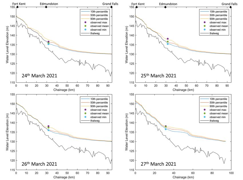
conditions can be used to simulate hundreds of probable ice jam scenarios. For example, as the location of ice
jams are difficult to predict during spring breakup, a range of ice jam locations can be used as model input.
Lindenschmidt et al. (2019) applied this approach in an operational flood forecasting context to predict maximum
probable ice jam water level elevations along the Athabasca River at Fort McMurray, Canada.
The main purpose of this study is to develop a stochastic modelling framework for an operational real-time ice-jam
flood forecasting system along the Saint John River, Canada. The specific objectives are i) to provide an ice-jam
flood outlook for spring ice-cover breakup and ii) to forecast probable maximum ice-jam backwater level
elevations.
2. Methodology
2.1 Study Area
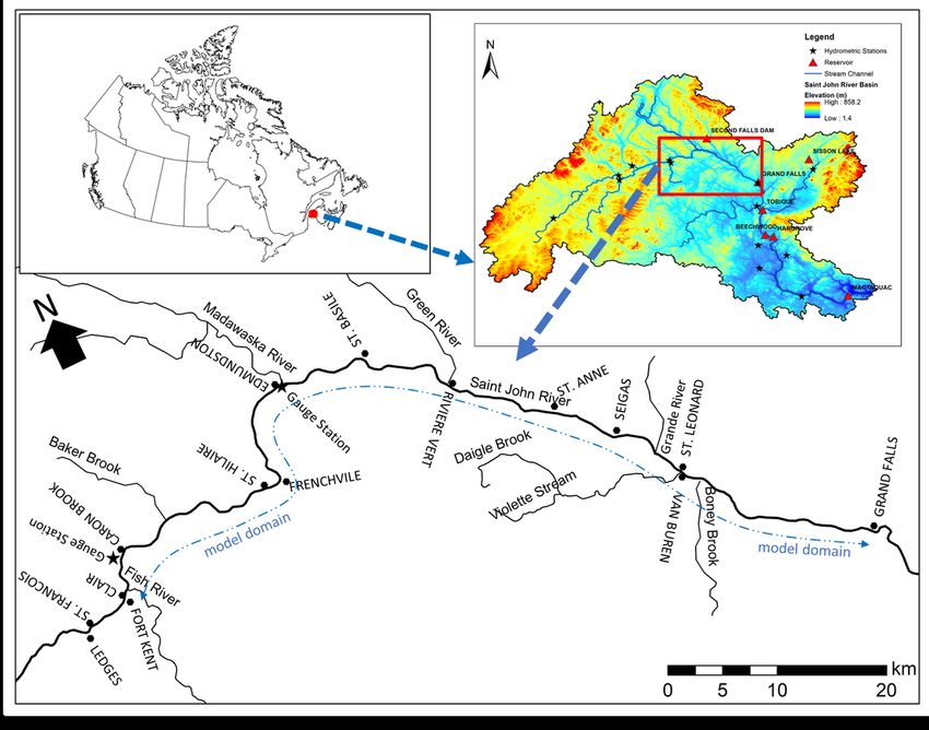
The hydrological model setup to simulate flows along the Saint John River extends across the Saint John River
Basin. This basin is situated in northeastern North America (Fig. 1), covering more than 55,000 km2 across the
United States and Canada. While a major portion of the basin is located in Canada (51% and 13% in the provinces
of New Brunswick and Quebec, respectively), the remaining portion (36%) is situated in the State of Maine, USA
(Kidd et al., 2011). The Saint John River is more than 700 km long, flows from northern Maine, USA to western New
Brunswick, Canada, before draining into the Bay of Fundy at Saint John, Canada. The total elevation drop of the
river is about 480 m (Beltaos et al., 2012).
The Saint John River basin has mixed humid continental and maritime climates (Kidd, Curry and Munkittrick,
2011). The average annual precipitation is measured to be 1100 mm, in which 30% is snowfall (Beltaos et al.,
2012). The mean annual discharge is approximately 1100 m3/s with a peak flow condition in later spring. The soil
type in the basin is dominated by “forest soil” - humo-ferric podzols and gray luvisols. The land cover mostly
consists of forests (70%), with some patches of cropland (6%) and wetlands (6%). There are three large
hydroelectric reservoirs in the basin, impounded by the Grand Falls, Beechwood and Mactaquac dams. Since there
is currently no active hydrometric station in the main river channel downstream of Fredericton hence the outlet
station for the hydrological model of the basin was taken to be at the Mactaquac Dam, which reduces the
hydrological model domain area to 41,000 km2.
The hydraulic model domain extends from Fort Kent to Grand Falls, an approximate 94 km long river reach. This
portion of the river is prone to ice jam formation during spring breakup due to its geomorphological settings. The
reach from Fort Kent to Edmundston is relatively steep with a series of rapids. The strech from Edmundston to
Grand Falls has a relatively milder slope, shallow riverbed, and many islands and sandbars that splits the main
river channels into multiple sub-channels.
Some hydraulic gauge stations record daily river flows and water levels along the study site. The United States
Geological Survey (USGS) operates the gauging stations at Dickey and Fort Kent, ECCC’s Water Survey of Canada
operate the gauge at Edmundston and New Brunswick Power own the gauge at Grand Falls. The hydrological
model is calibrated and validated using streamflow records from Dickey and Grand Falls. Since the hydraulic
model was calibrated and validated using the water levels recorded at the Edmundston gauge station and the
model simulates ice jam backwater level profiles, the model framework was developed to forecast the severity of
ice jams downstream of Edmundston.
Page 3/19
2.2 MESH hydrological model
MESH is a physically-based hydrological land-surface model from Environment and Climate Change Canada
(ECCC) (Pietroniro et al., 2007) and has been widely used in different parts of Canada, from small to large
catchments (Mengistu & Spence, 2016; Haghnegahdar et al., 2017; Yassin et al., 2017; Lindenschmidt et al., 2019;
Budhathoki et al., 2020; Rokaya et al., 2020). MESH uses a grouped response unit (GRU) approach to capture basin
heterogeneity. It has a grid-based modelling system which is composed of three major components (i) a vertical
exchange of water within a grid cell between the land surface and the atmosphere (ii) the routing of lateral fluxes
and (iii) the generation of surface and sub-surface runoff. MESH uses the Canadian Land Surface Scheme
(CLASS) (Verseghy, 1991) for the vertical generation and exchange of lateral fluxes. WATROF (Soulis et al., 2000)
and PDMROF (Mekonnen et al., 2014) are the two scheme used to account for lateral fluxes. The routing of surface
and subsurface runoff is performed using WATROUTE (Kouwen, 2016).
2.3 Meteorological Input for MESH
MESH requires seven meteorological forcing inputs: precipitation, wind speed, air temperature, specific humidity,
incoming longwave radiation, barometric pressure and incoming shortwave radiation. For model calibration and
validation, all inputs except precipitation were taken from combined gridded datasets of Global Environmental
Multiscale (GEM) model (Côté et al., 1998; Yeh et al., 2002) which is available at an hourly temporal resolution and
at the spatial resolution of 15 km. The precipitation inputs were taken from the Canadian Precipitation Analysis
(CaPA) (Mahfouf et al., 2007) datasets which are available at 6 hour time intervals at a spatial resolution of 10 km.
CaPA is found to be a reliable precipitation product for the Canadian domain (Boluwade et al., 2018).

For streamflow forecasting, all the meteorological forcing data were retrieved from Global Deterministic Prediction
System (GDPS). GDPS is an operational forecasting system, based on the GEM model from ECCC which provides
deterministic predictions of atmospheric variables with a 10-day lead time (Bélair et al., 2009; Charron et al., 2012).
The forecasts are produced two times a day (00 UTC and 12 UTC) at 3-hourly temporal resolution and has an
approximate 25 km spatial resolution.
2.4 MESH set up and calibration
“The topographic data for SJRB were obtained from the hydrologically adjusted elevation of MERIT Hydro which is
at a resolution of 3 arc-second resolution (~ 90 m at the equator) (http://hydro.iis.u-
tokyo.ac.jp/~yamadai/MERIT_Hydro/) (Yamazaki et al., 2019).The landcover data were derived from the
Commission for Environmental Cooperation (CEC) land cover database in 30 m resolution
(http://www.cec.org/north-american-environmental-atlas/land-cover-2010-landsat-30m/). The vegetation
parameters were obtained from literature (Kidd et al., 2011) and the CLASS manual (Verseghy, 2009) and the soil
texture information was obtained from the Unified North American Soil Map (UNASM) (LIU et al., 2014) for
different soil depths.” (Budhathoki et al., submitted). Six vertical soil profile layers of 10 cm, 35 cm, 120 cm, 260
cm, 310 cm and 410 cm were defined from the surface boundary in MESH. The model was built with a grid
resolution of 0.125 deg. (approx. 10 km), resulting in 373 grid cells. Nine GRUs were created based on the
landcover variability in the basin. The preprocessing of the spatial data was conducted using ECCC’s Green Kenue
software (EnSim Hydrologic, 2014) to generate drainage networks and other topographically driven basin
characteristics such as slope and channel length. The discharge data were retrieved from ECCC’s database HYDAT
and the reservoir inflows and outflows were retrieved from the New Brunswick Power company.
                                                       Page 4/19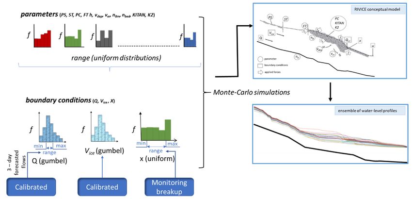
The calibration was performed using parallel DDS algorithm in OSTRICH (Matott, 2005) with the Nash Sutcliffe
Efficiency (NSE) as the objective function. The sensitive parameters were selected based on Haghnegahdar et al.
(2017) and ten parameters of six dominant GRU’s were calibrated. The model was calibrated for the period 2002–
2010 considering the first year (Oct 2002 - Oct 2003) as the model spin-up period. The validation was then
performed using the subsequent six years (2011–2018).

2.5 Streamflow Forecast
Forecasting the basin’s streamflow involves a two-step process, first running the MESH model in hindcast mode,
which saves the state variables until the previous day (yesterday) of the forecast period and then performing the
flow forecast for the next 10 days (from today) with the saved state variables. It is important to save and update
the basin state variables and hydrologic conditions everyday so that the initial hydrologic conditions for running
the model are always accurate. Figure 2 shows the schematic view of the MESH operational forecasting setup for
the SJRB.

In the hindcasting mode, the forcing data for precipitation were obtained from CaPA and other meteorological
forcing data were retrieved from the GEM system. In the forecasting mode, all the meteorological forcing data were
retrieved from the GDPS system. MESH was run at an hourly time step in the hindcasting mode and 3-hourly in the
forecasting mode to match the temporal resolution of the meteorological data.

2.6 RIVICE hydraulic model
RIVICE is a one-dimensional hydrodynamic model that simulates various river ice phenomena, including the
formations of frazil ice, border ice, solid ice covers and ice jams. RIVICE solves the Saint Venant equations for
transient flows and water levels using an implicit finite difference scheme. A user usually calibrates the time steps
and appropriate lengths of the simulation based on specific sites and purposes. Surveyed cross-sections are the
primary inputs to set up the model structure along a river. Moreover, the model requires various hydraulic and river
ice parameters and boundary condition inputs to simulate these processes. A conceptual diagram of ice jam
simulations and their require variables is shown in Fig. 3. Some of these parameters and boundary conditions are
user-defined or calibrated based on historical events along the model domain. Table I briefly describes all of the
parameters and boundary conditions. For further details about the RIVICE the reader may refer to the online
manual (http://giws.usask.ca/rivice/Manual/RIVICE_Manual_2013-01-11.pdf) and to Lindenschmidt (2017).

Table I Description of RIVICE parameters and boundary conditions

                                                      Page 5/19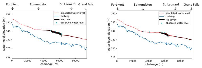
Inputs                  Description                             Units

                     Boundary Conditions

                     Q                       Upstream river discharge                m3/s

                     W                       Downstream water level                  m a.s.l

                     Vice                    Inflowing volume of ice                 m3

                     x                       Toe of the ice-jam location             none

                     Parameters

                     PC                      Porosity of ice-cover                   none

                     FT                      Thickness of ice-cover                  m

                     PS                      Porosity of slush pans                  none

                     ST                      Thickness of slush pans                 m

                     vdep                    ice deposition velocity                 m/s

                     ver                     ice erosion velocity                    m/s

                     nbed                    Riverbed roughness                      s/m⅓

                     n8m                     ice roughness                           s/m⅓

                     K1                      Longitudinal to lateral force ratio     none

                     K2                      longitudinal to vertical force ratio    none

                     h                       Thickness of ice downstream of jam      m

2.7 Stochastic framework for forecasting
In the stochastic framework (Fig. 4), the RIVICE hydrodynamic model is placed within a Monte-Carlo Analysis
(MOCA) framework to simulate hundreds of ice jam scenarios using randomly selected sets of parameters and
boundary conditions. To select random values of the parameters and boundary conditions, minimum and
maximum values of the inputs were extracted from gauge records and the calibration data of previous studies
along the model domain. While the uniform distribution of most of the parameters and toe of ice jam location are
used to select the random values for the MOCA, an extreme value distribution (Gumbel) was implemented for two
important boundary conditions – river discharge and the inflowing volume of ice.

An extreme value distribution was developed for river discharge using observed flows recorded at the Fort Kent
gauging station during spring breakup. The location and scale parameters of the distribution were then used to
select the random values from the maximum and minimum range of forecasted flows. The 3-day probable
streamflow data from the MESH hydrological model was used to select the maximum and minimum range of the
flows. The lateral flow inputs from various major tributaries along the model domain were also estimated by
establishing linear relationships between the Fort Kent discharge and tributary flows.

                                                    Page 6/19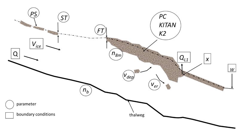
The observed flow frequency distribution during spring breakup was used as an input in the MOCA framework. The
volume-of-ice frequency distribution was then calibrated by comparing (i) the frequency distribution of the
ensemble of stages simulated at Edmundston and (ii) the frequency distribution of the water level elevations
recorded at the Edmundston gauge during ice-jam events. If the two distributions did not coincide, the volume-of-
ice frequency distribution was adjusted and the MOCA repeated to yield a new “simulated” frequency distribution
of stages at Edmundston for comparison, again, with the “observed” frequency distribution of the water level
elevations recorded at Edmundston. The process is repeated until the “simulated” and “observed” frequency
distributions of the volume of ice consistently coincided. A more detailed description of this process can be
obtained from Lindenschmidt (2020; p. 181–183).

Once all the parameters and boundary conditions distributions were established, the framework was used to
produce a seasonal outlook (before the breakup initiation along the model domain) of the severity of ice jam from
22 March 2021. The 3-day forecasting simulation began on 24 March 2021. Additional information was updated
using the New Brunswick government’s daily interactive map of ice observation, especially important to track the
toe of ice jam location.

3. Result And Discussion
3.1 MESH calibration and validation
The results of the MESH calibration and validation for the gauging station 01AF002 (Saint John River at Grand
Falls) is shown in Fig. 5. The observed and simulated flows are in good agreement with each other. The NSE value
of 0.89 and log (NSE) value of 0.84 were achieved for the calibration period whereas for the validation period,
values of NSE = 0.88 and log(NSE) = 0.85 were obtained.
3.2 MESH 10-day flow forecasts
10-day flow forecasts were simulated using MESH. Figure 6 shows the flow forecast at the Fort Kent station during
the spring of 2021. MESH was able to forecast the timing of the rise in the flows with a Pbias of + 15 % (based on
the average of a seven-day daily forecast). The forecasted flow data from these events are used as an important
boundary condition to assist parallel ice-jam forecasting.

3.4 RIVICE calibration and validation
The RIVICE model is calibrated and validated using historical ice jam events in 1991 and 2008 along the Saint
John River. Observed water level and related data of these events were obtained from the study by Beltaos et al.
(2012). First hydraulic and river ice parameters were calibrated until good agreement was obtained between
simulated and observed water level profiles. Figure 7 (left panel) shows the RIVICE calibration result for the ice jam
event of 1991 that occurred upstream of St. Leonard. To validate the model, the same calibration data were used
to simulate the ice jam that occurred in 2009. Figure 7 (right panel) shows a good agreement between observed
and simulated water levels of the 2009 ice jam event.

3.5 Ice cover breakup in spring 2021

                                                      Page 7/19
Spring ice cover breakup in 2021 was triggered by consistent warm air temperatures (above 0ºC) from 20 to 25
March 2021. During this period, river discharge increased significantly from 124 to 1241 m3/s due to rapid
snowmelt (Fig. 8). By 24 March 2021, ice covers began to crack and melt out forming open-water leads in the ice
cover. On 25 March 2021, a long open-water section with intermittent fragmented ice was observed from
downstream of Frenchville to Grand Isle. The ice cover from Fort Kent to Edmundston completely broke up with ice
moving downstream of Edmundston by 26 March 2021. On 27 March 2021, an ice jam formed immediately
upstream of Sainte-Anne-de-Madawaska, which extended upstream for more than 20 km by 28 March 2021. On
this day, the water level elevation at Edmundston gauge station increased to the season maximum of 138.126 m
a.s.l.

3.6 Ice jam flood outlook for spring 2021
The main goal of the ice jam flood outlook is to provide a preliminary forecast for the breakup period. Since MESH
usually simulates 10-day flow forecasts, the outlook results present the potential maximum ice-jam water level
profiles for the next 10 days. Figure 9 shows the ice-jam flood outlook from 22 to 31 March 2021. The outlook
predicted the maximum water level elevation due to ice jam formation to be lower than the flood level (140.5 m
a.s.l according to the New Brunswick Government river watch website). The comparison between observed water
level and simulated water level profiles shows that the simulated outlook (90th percentile) was fairly accurate to
predict maximum water level elevations.
3.7 Ice jam flood forecasting during spring 2021
The 3-day ice jam flood forecasts began on 24 March 2021. Each day a total of 250 ice jam scenarios were
simulated in the stochastic modelling framework to predict the severity of ice jam flooding along the study site.
Figure 10 shows the forecasting results from 24 to 27 March 2021, indicating the 10th, 50th, and 90th percentiles
of the ice jam water level profiles. As the ice cover was still intact on 24 March, the simulations slightly
overestimated the water level elevations along the river. The forecasting results started to improve when the ice
cover broke up from 25 to 27 March 2021. The ice jam flood forecast from 27 March 2021compares well with the
observed water level elevations at the Edmundston gauge. The results show that the mean and maximum
observed water level elevations at Edmundston were within the 50th and 90th percentiles of the forecasted water
level profiles. Overall, the 3-day flood forecasting was effective to estimate the backwater level conditions during
breakup.

4. Potential Sources Of Error
Although the stochastic approach for ice jam flood forecasting provides a reasonable outcome to predict the
severity of flooding, there are still some limitations and uncertainties associated with the assumptions and
parameter selection.

- the volume of inflowing ice has been calibrated and selected as an independent parameter, which may not always
be the case, as this variable depends on streamflow conditions. For example, low spring flow conditions may result
in thermal breakup and significant ice melt, leading to relatively small ice volumes to form ice jams. The opposite
is true for the high spring flows, however in this stochastic approach the model simulation can be incorporated
with high flows with low volumes to mimic under-developed ice jams. Moreover, these uncertainties can also be
associated with the errors in the selected parameter distributions.

                                                      Page 8/19
- the toe of the ice-jam location is not always uniformly distributed along the river and there are some preferred ice-
lodgment sites. Although the study was used observed ice breakup and potential ice jam toe locations, there are
still some discrepancies between forecasting setup and observed information. Hence the incorrect selection of toe
location range can create an additional error in the forecasting results.
- tribuatary inflows in the model domain were considered as a mean flow, which may not reflect the actual river
flow condition. Since the hydrological model forecasting setup only provides the upstream flow conditions of the
main model domain, providing tributary flows dynamically would not decrease the overall error.
- the study considered the peak breakup water level due to ice-jam formation along the river stretch downstream of
Edmundston; therefore the results were only validated using the observed water level recorded at the Edmundston
gauge station. Therefore, there are maybe some biases that should be considered to assess the forecasting
results.
5. Conclusion
A stochastic modelling framework was developed to forecast the severity of ice jam flooding along the Saint John
River from Fort Kent to Grand Falls. The framework loosely coupled a hydrological land-surface model MESH with
a hydrodynamic river ice model RIVICE to simulate hundreds of probable ice jam scenarios using a Monte-Carlo
analysis.
Within this stochastic framework, an outlook was provided at the beginning of the breakup to assess the 10-day
ice jam severity along the study site. This is one of the novelties in the field of ice jam flood forecasting. This
outlook may help to provide early warning and extra preparation time to improve mitigation strategies. The 3-day
ice jam flood forecasting was also able to simulate maximum water levels more accurately. Overall, the framework
can be used in real-time mode for operations ice-jam flood forecasting and mitigation management and planning.
6. Declarations
Ethical Approval
Not Applicable
Consent to Participate
Not Applicable
Consent to Publish
Not Applicable
Authors Contributions
AD carried out all the data analyses and wrote most of the sections of the manuscript. SB provided hydrological
model results and wrote some sections of the manuscript. KEL conceptually helped to develop the paper and
reviewed the manuscript throughout the process.
Funding
Page 9/19Global Water Future, Global Institute for Water Security, University of Saskatchewan
Competing Interests
None
Data Availability Statement
The historical hydrometric and meteorological data are available from Environment and Climate Change Canada
and Unites State Geological Survey (USGS). The model simulated data and code are available from the
corresponding author upon reasonable request.
Conflict of Interest
None
Acknowledgement
The authors thank the University of Saskatchewan’s Global Water Future program at the Global Institute for Water
Security for their funding support of this research. Thanks also go to New Brunswick Power for the water levels
and flows recorded at Grand Falls.
7. References
1. Beltaos, S. (2002). Effects of climate on mid‐winter ice jams. Hydrological Processes, 16(4), 789-804.
2. Beltaos, S. (2004). Climate impacts on the ice regime of an Atlantic river. Hydrology Research, 35(2), 81-99.
3. Bélair, S., Roch, M., Leduc, A.-M., Vaillancourt, P. A., Laroche, S., & Mailhot, J. (2009). Medium-range
quantitative precipitation forecasts from Canada’s new 33-km deterministic global operational system.
Weather and forecasting, 24(3), 690-708.
4. Beltaos, S., Tang, P., & Rowsell, R. (2012). Ice jam modelling and field data collection for flood forecasting in
the Saint John River, Canada. Hydrological Processes, 26(17), 2535-2545.
5. Boluwade, A., Zhao, K.-Y., Stadnyk, T. A., & Rasmussen, P. (2018). Towards validation of the Canadian
precipitation analysis (CaPA) for hydrologic modeling applications in the Canadian Prairies. Journal of
Hydrology, 556, 1244-1255.
6. Budhathoki, S., Rokaya, P., & Lindenschmidt, K.-E. (2020). Improved modelling of a Prairie catchment using a
progressive two-stage calibration strategy with in situ soil moisture and streamflow data. Hydrology Research,
51(3), 505-520.
7. Charron, M., Polavarapu, S., Buehner, M., Vaillancourt, P., Charette, C., Roch, M., . . . MacPherson, S. (2012). The
stratospheric extension of the Canadian global deterministic medium-range weather forecasting system and
its impact on tropospheric forecasts. Monthly Weather Review, 140(6), 1924-1944.
8. Côté, J., Gravel, S., Méthot, A., Patoine, A., Roch, M., & Staniforth, A. (1998). The operational CMC–MRB global
environmental multiscale (GEM) model. Part I: Design considerations and formulation. Monthly Weather
Review, 126(6), 1373-1395.
9. Das, A. (2021). Stochastic modelling approach to improve ice-jam flood risk management (Doctoral
dissertation, University of Saskatchewan).
Page 10/1910. Doyle, P. F. (2009). Beltaos, Spyros (Editor). 2008. River Ice Breakup. Canadian Water Resources Journal, 34(1),
95-97.
11. Haghnegahdar, A., Razavi, S., Yassin, F., & Wheater, H. (2017). Multicriteria sensitivity analysis as a diagnostic
tool for understanding model behaviour and characterizing model uncertainty. Hydrological Processes, 31(25),
4462-4476.
12. Humes, T. M., & Dublin, J. (1988). A comparison of the 1976 and the 1987 St. John River ice jam flooding with
emphasis on antecedent conditions. In Proceedings of the Workshop on Hydraulics of River Ice/Ice Jams (pp.
43-62).
13. Kidd, S D, R A Curry, and K R Munkittrick. The Saint John River: A State of the Environment Report. Fredericton,
New Brunswick, Canada: Canadian River Institute - University of New
Brunswick,2011. https://www.unb.ca/research/institutes/cri/_resources/pdfs/criday2011/cri_sjr_soe_final.pdf
14. Kouwen, N. (2016). WATFLOOD/WATROUTE Hydrological Model Routing and Flood Forecasting System,
User's Manual: University of Waterloo, Waterloo, ON.
15. Lindenschmidt, K.-E., Rokaya, P., Das, A., Li, Z., & Richard, D. (2019). A novel stochastic modelling approach for
operational real-time ice-jam flood forecasting. Journal of Hydrology, 575, 381-394.
16. Lindenschmidt, K.-E. (2020) River ice processes and ice flood forecasting – a guide for practitioners and
students. Springer Nature Switzerland AG. 267 pp. https://doi.org/10.1007/978-3-030-28679-8
17. Lindenschmidt, K.-E. (2017). RIVICE—a non-proprietary, open-source, one-dimensional river-ice model. Water,
9(5), 314.
18. LIU, S., Wei, Y., Post, W., Cook, R., Schaefer, K., & Thornton, M. (2014). NACP MsTMIP: Unified North American
Soil Map. ORNL DAAC.
19. Mahfouf, J. F., Brasnett, B., & Gagnon, S. (2007). A Canadian precipitation analysis (CaPA) project: Description
and preliminary results. Atmosphere-ocean, 45(1), 1-17.
20. Matott, L. S. (2005). OSTRICH: An optimization software tool: Documentation and users guide. University at
Buffalo, Buffalo, NY.
21. Mekonnen, M., Wheater, H., Ireson, A., Spence, C., Davison, B., & Pietroniro, A. (2014). Towards an improved
land surface scheme for prairie landscapes. Journal of Hydrology, 511, 105-116.
22. Mengistu, S., & Spence, C. (2016). Testing the ability of a semidistributed hydrological model to simulate
contributing area. Water Resources Research, 52(6), 4399-4415.
23. Pietroniro, A., Fortin, V., Kouwen, N., Neal, C., Turcotte, R., Davison, B., . . . Evora, N. (2007). Development of the
MESH modelling system for hydrological ensemble forecasting of the Laurentian Great Lakes at the regional
scale. Hydrology and Earth System Sciences, 11(4), 1279-1294.
24. Rokaya, P., Wheater, H., & Lindenschmidt, K.-E. (2019). Promoting sustainable ice-jam flood management
along the Peace River and Peace-Athabasca Delta. Journal of Water Resources Planning and Management,
145(1), 04018085.
25. Rokaya, P., Peters, D. L., Elshamy, M., Budhathoki, S., & Lindenschmidt, K. E. (2020). Impacts of future climate
on the hydrology of a northern headwaters basin and its implications for a downstream deltaic ecosystem.
Hydrological Processes, 34(7), 1630-1646.
26. Soulis, E. D., Snelgrove, K. R., Kouwen, N., Seglenieks, F., & Verseghy, D. L. (2000). Towards closing the vertical
water balance in Canadian atmospheric models: coupling of the land surface scheme CLASS with the
distributed hydrological model WATFLOOD. Atmosphere-ocean, 38(1), 251-269.
Page 11/1927. Tang, P., & Beltaos, S. P. Y. R. O. S. (2008, May). Modeling of river ice jams for flood forecasting in New
Brunswick. In Proceedings, 65th Eastern Snow Conference (pp. 167-178). Fairlee (Lake Morey) Vermont, USA,
Bridgewater State College and ERDC-CRREL.
28. Williams, B. S., Das, A., Johnston, P., Luo, B., & Lindenschmidt, K.-E. (2021). Measuring the skill of an
operational ice jam flood forecasting system. International Journal of Disaster Risk Reduction, 52, 102001.
29. Yamazaki, D., Ikeshima, D., Sosa, J., Bates, P. D., Allen, G. H., & Pavelsky, T. M. (2019). MERIT Hydro: a high‐
resolution global hydrography map based on latest topography dataset. Water Resources Research, 55(6),
5053-5073.
30. Yassin, F., Razavi, S., Wheater, H., Sapriza‐Azuri, G., Davison, B., & Pietroniro, A. (2017). Enhanced identification
of a hydrologic model using streamflow and satellite water storage data: A multicriteria sensitivity analysis
and optimization approach. Hydrological Processes, 31(19), 3320-3333.
31. Yeh, K.-S., Côté, J., Gravel, S., Méthot, A., Patoine, A., Roch, M., & Staniforth, A. (2002). The CMC–MRB global
environmental multiscale (GEM) model. Part III: Nonhydrostatic formulation. Monthly Weather Review, 130(2),
339-356.
Figures
Page 12/19Figure 1
Study site including hydrological and hydraulic model domains of Saint John River and its basin.
Page 13/19Figure 2
Schematic view of MESH operational streamflow forecasting setup
Figure 3
A conceptual diagram of the ice jam modelling using RIVICE.
Page 14/19Figure 4
Stochastic framework for ice jam flood forecasting.
Page 15/19Figure 5
Observed and simulated flows at Grand Falls for the (a) calibration and (b) validation periods.
Page 16/19Figure 6
Forecast at Fort Kent (01AD002) for the spring breakup event in 2021.
Figure 7
RVICE calibration (left panel) and validation (right panel) results using historical ice jam events in 1991 and 2009
along the model domain (data sources: Beltaos et al. 2012)
Page 17/19Figure 8
Daily mean streamflow at Fort Kent gauging station and air temperatures at the Edmundston meteorological
station.
Page 18/19Figure 9
Ice jam flood outlook from 22 to 31 March 2021.
Figure 10
The 3-day ice jam flood forecasts from 24 to 27 March 2021 along the Saint John River from Fort Kent to Grand
Falls.
Page 19/19You can also read