Neural Process for Black-Box Model Optimization Under Bayesian Framework
←
→
Page content transcription
If your browser does not render page correctly, please read the page content below
Neural Process for Black-Box Model Optimization Under Bayesian Framework
                                                                     Zhongkai Shangguan,1 Lei Lin,2 Wencheng Wu,2 Beilei Xu2
                                                           12
                                                                Rochester Data Science Consortium, University of Rochester, Rochester, NY 14604 USA
                                                                  1
                                                                    zshangg2@ur.rochester.edu 2 {Lei.Lin, Wencheng.Wu, Beilei.Xu}@rochester.edu
arXiv:2104.02487v1 [cs.LG] 3 Apr 2021

                                                                     Abstract                                reflect the current power system status, identify and miti-
                                                                                                             gate potential issues (Lin et al. 2020); geometric structure
                                          There are a large number of optimization problems in phys-         parameter optimization of an antenna aims at reaching an
                                          ical models where the relationships between model parame-
                                                                                                             optimal gain in working frequency band (Gustafsson 2016).
                                          ters and outputs are unknown or hard to track. These mod-
                                          els are named as “black-box models” in general because they        In many cases, this optimization process is done manually
                                          can only be viewed in terms of inputs and outputs, without         by experts based on a series of experiments. However, this
                                          knowledge of the internal workings. Optimizing the black-          process requires expert domain knowledge and a number of
                                          box model parameters has become increasingly expensive             experiments to be conducted, which can be both expensive
                                          and time consuming as they have become more complex.               and time consuming. In order to reduce human effort and
                                          Hence, developing effective and efficient black-box model          the number of required experiments, automated optimiza-
                                          optimization algorithms has become an important task. One          tion algorithms with varying computational complexity and
                                          powerful algorithm to solve such problem is Bayesian opti-         scalability have been proposed.
                                          mization, which can effectively estimates the model parame-
                                          ters that lead to the best performance, and Gaussian Process          Conventional automated black-box model optimization
                                          (GP) has been one of the most widely used surrogate model          algorithms include grid search and random search (Bergstra
                                          in Bayesian optimization. However, the time complexity of          and Bengio 2012). In grid search, the problem is defined in
                                          GP scales cubically with respect to the number of observed         a high-dimensional grid space where each grid dimension
                                          model outputs, and GP does not scale well with large pa-           corresponds to a parameter, and each grid point corresponds
                                          rameter dimension either. Consequently, it has been challeng-      to a parameter combination. We then evaluate the model on
                                          ing for GP to optimize black-box models that need to query         all parameter combinations defined by the grids, and select
                                          many observations and/or have many parameters. To over-            the parameter combination that yields the best performance
                                          come the drawbacks of GP, in this study, we propose a general      of the model. One drawback of grid search is that the num-
                                          Bayesian optimization algorithm that employs a Neural Pro-
                                          cess (NP) as the surrogate model to perform black-box model
                                                                                                             ber of grid points grows exponentially as the number and
                                          optimization, namely, Neural Process for Bayesian Optimiza-        value range of the parameters increase. On the other hand,
                                          tion (NPBO). In order to validate the benefits of NPBO,            random search approach can potentially explore the param-
                                          we compare NPBO with four benchmark approaches on a                eter space more extensively through randomly generates pa-
                                          power system parameter optimization problem and a series           rameter combinations in the parameter space. However, both
                                          of seven benchmark Bayesian optimization problems. The re-         of these two methods do not utilize the prior sampled in-
                                          sults show that the proposed NPBO performs better than the         formation, so that the search is blind. Recently, more ad-
                                          other four benchmark approaches on the power system pa-            vanced automated optimization algorithms have been intro-
                                          rameter optimization problem and competitively on the seven        duced, including evolutionary optimization (Cheng 2018),
                                          benchmark problems.                                                population-based optimization (Jaderberg et al. 2017), and
                                                                                                             Bayesian optimization (Frazier 2018). These algorithms
                                                                  Introduction                               construct the relationship between parameter combinations
                                                                                                             and the performance of black-box models, and provide guid-
                                        A complex physical model can be viewed as a black-box                ance for the next selection of parameter combination for
                                        model since it can only be viewed in terms of its inputs (pa-        evaluation, which make those methods more efficient to find
                                        rameters) and outputs (observations) when internal workings          the global optimal parameter combination.
                                        are hard to track. Optimizing the parameters of such a black-
                                                                                                                In this paper, we focus on the Bayesian optimization
                                        box model is a common problem in engineering fields (Xiao
                                                                                                             framework. Bayesian optimization implements a surrogate
                                        et al. 2015; Cassioli 2013; Zhang and Zhang 2010). For ex-
                                                                                                             model that predicts the black-box model performance for a
                                        amples, power system models need regular calibrations to
                                                                                                             specific parameter combination; and an acquisition function,
                                        Copyright © 2021, for this paper by its authors. Use permitted un-   which trades off exploration and exploitation to query the
                                        der Creative Commons License Attribution 4.0 International (CC       next observation point. An accurate surrogate model that can
                                        BY 4.0)                                                              predict the black-box model performance as well as measure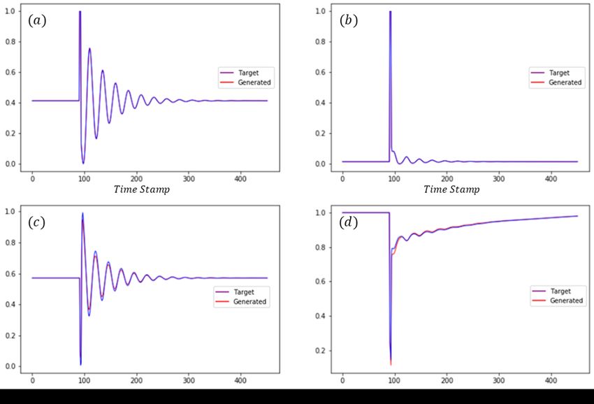
the uncertainty is crucial to the performance of Bayesian op-    Rd → R. It can be formulated as (1):
timization. Gaussian process (GP) has been the most widely
used surrogate model for Bayesian optimization (Rasmussen                               x̂ = argmax f (x),                          (1)
                                                                                            x∈A⊂Rd
and Williams 2006) due to its expressiveness, smoothness
and well-calibrated uncertainty estimation of the model re-      where d is the dimension of x, A is the constrain that de-
sponse. However, GP has O(N 3 ) time complexity, where N         fined for f (x), f (·) is the nonlinear function that is expen-
is the number of training samples (Rasmussen and Williams        sive to evaluate, and x̂ is the estimation of the input param-
2006), so it is computationally expensive. Another drawback      eter. One assumption of Bayesian optimization is that only
of GP is its poor scalability to high parameter dimensions       the outputs f (x) can be observed while its derivatives can-
(Liu et al. 2020), i.e., with the increase in the dimension of   not be obtained. Hence, f (·) is a black-box model and the
parameters, the performance of GP becomes worse. Hence,          optimization problem cannot be solved using gradient de-
GP cannot be applied to problems that require to query many      scent algorithm. Bayesian optimization repeatedly executes
observations and/or have many parameters.                        the following steps until a satisfactory input parameter com-
   To overcome these issues, we propose a new algorithm          bination is found: (i) fit a surrogate model to the current ob-
for black-box model optimization by employing Neural Pro-        servations to get a prior distribution; (ii) convert the prior
cess as a powerful and scalable surrogate model under the        to the posterior distribution and predict where the next in-
Bayesian optimization framework, namely, Neural Process          put parameter combination is by maximizing an acquisition
for Bayesian Optimization (NPBO). Neural Process (NP)            function; (iii) obtain the observation on the suggested pa-
(Garnelo et al. 2018b) is an algorithm to simulate stochastic    rameter combination and add the result to the observation
process using neural networks (NNs). It combines the ad-         set. The third step is usually the most expensive step since
vantages of stochastic process and NNs so that it has the        it needs to generate the observation on the expensive black-
ability to capture uncertainty while predicting the black-box    box model.
model’s performance accurately. The performance of the              There are two main components in Bayesian optimiza-
proposed algorithm is evaluated on a power system param-         tion: a surrogate model that simulates the black-box model
eter optimization problem and seven benchmark problems           and an acquisition function that trades off exploration and
for Bayesian optimization (Klein et al. 2017). The results       exploitation in order to decide the next query inputs. GP
show that the proposed NPBO outperforms the other four           is a classical model that is widely employed as the sur-
benchmark approaches including GP-based Bayesian opti-           rogate model by Bayesian optimization. A GP is defined
mization, random forest based Bayesian optimization, Deep        as a stochastic process indexed by a set X ⊆ Rd :
Networks for Global Optimization (DNGO) and Bayesian             {f (x) : x ∈ X } such that any finite number of random vari-
Optimization with Hamiltonian Monte Carlo Artificial Neu-        ables of the process has a joint Gaussian distribution. Instead
ral Networks (BOHAMIANN) on the power system parame-             of inferring a distribution over the parameters, GP can be
ter optimization problem and performs competitively on the       used to infer a distribution over the function directly. For ex-
benchmark problems.                                              ample, considering we sample a finite set D = {x1 , ..., xn },
   The rest of the paper is arranged as follows. Related         D ∈ X , GP is completely defined by its mean and covari-
Work introduces state-of-the-art methods in parameter op-        ance functions as (2) shows
timization under the Bayesian optimization framework. The
methodology of NPBO is introduced in detail in Methodol-                            p(f |D) = N (f |µ, K)                           (2)
ogy. We compare and discuss the results of NPBO and the          where f = (f (x1 ), ...f (xn )) is the distribution over the
benchmark algorithms in the Experiment section. Finally,         black-box model; µ = (m(x1 ), ..., m(xn )) where m is the
the paper concludes our work and discusses future steps.         mean function, and K = K(xi , xj ) represents the covari-
                                                                 ance function (also known as kernel) such as Radial basis
                     Related Work                                function kernel (Görtler, Kehlbeck, and Deussen 2019). So
This section will introduce the framework of Bayesian op-        for a specific x, GP predicts a mean and a variance that
timization using GP, then discuss previous proposed ap-          completely define a Gaussian distribution over f (x), i.e.,
proaches (Snoek et al. 2015; Springenberg et al. 2016) that      f (x) ∼ N (f (x)|m(x), K(x)).
use NNs as alternative surrogate models.                            Expected improvement (EI) is one of the popular acquisi-
                                                                 tion functions in Bayesian optimization (Frazier 2018). EI is
Bayesian Optimization Framework                                  computed as the expectation taken with respect to the poste-
                                                                 rior distribution. It is defined as:
Bayesian optimization is a state-of-the-art optimization
framework for black-box model optimization problems. It           αEI (x) :=
has great power in parameter optimization of physical mod-

                                                                                        µ(x) − τ                     µ(x) − τ       (3)
els (Duris et al. 2020; Muehleisen and Bergerson 2016) and           (µ(x) − τ )Φ                      + σ(x)φ
                                                                                          σ(x)                         σ(x)
hyperparameter optimization in training machine learning
(ML) models (Chen et al. 2018). A detailed tutorial can be       where Φ and φ represent the cumulative distribution func-
found in (Archetti and Candelieri 2019).                         tion and probability distribution function of standard normal
   The aim of Bayesian optimization is to find the input         distribution, τ is the current best observed outcome, µ and σ
x that maximizes an unknown nonlinear function f (x) :           are the mean and variance.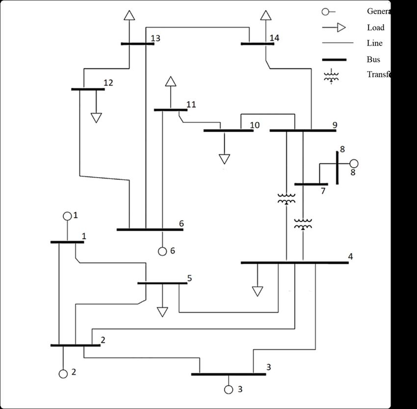
Bayesian Optimization with Neural Networks                       Neural Process for Bayesian Optimization
                                                                 NP is a neural network based approach to represent a dis-
To address the downsides of the standard GP, i.e., scal-         tribution over functions. It builds neural networks to model
ing cubically with the number of queried observations and        functions as a random process f . Given a set of observa-
not performing well with high dimensional data, alternative      tions ((x1 , y1 ), ..., (xN , yN )), NP first defines ρx1:N as the
methods based on sparse GP approximations (Snelson and           marginal distribution of (f (x1 ), ..., f (xN )), i.e.
Ghahramani 2006; Lázaro-Gredilla et al. 2010; McIntire,
Ratner, and Ermon 2016) have been proposed. These meth-                       ρx1:N (y1:N ) := ρx1 ,...,xN (y1 , ..., yN )                   (4)
ods approximate the full GP by using subsets of the orig-        Assuming that the independence among samples and obser-
inal dataset as inducing points to build a covariance func-      vation noise exists, i.e. yi = f (xi )+εi ∼ N (f (xi ), σ 2 (xi )),
tion. However, they are not accurate in uncertainty estima-      in order to build a model on (4), the conditional distribution
tion and still have poor scalability in high dimensional pa-     can be written as
rameter space (Hebbal et al. 2019). Since NNs are very flexi-
                                                                                                     N
ble and scalable, adapting NNs to the Bayesian optimization                                          Y
framework is highly desirable. However, NNs are determin-                 p(y1:N |x1:N , f ) =             N (yi |f (xi ), σ 2 (xi ))        (5)
istic models that do not have the ability to measure the un-                                         i=1
certainty. Hence, combining the flexibility and scalability of   where p denotes the probability distribution. Then, in order
NNs with well-calibrated uncertainty estimations is crucial      to build the stochastic process f using neural network, we
in this procedure.                                               assume f (x) = g(x, z), where z is a latent vector that is
   More recently, Bayesian optimization methods based on         sufficient to represent f , and g is a general function defined
NNs have been proposed. Snoek et al. (2015) propose a            for f . We assume p(z) obeys a multivariate standard nor-
Deep Networks for Global Optimization (DNGO) frame-              mal, then the random process f becomes sampling of z. For
work that uses NNs as the feature extractor to pre-process       example, assuming f is a GP, then z should be a vector con-
the inputs, and then adapts a Bayesian linear regression         taining the mean and variance that can fully define the GP.
(BLR) model to gain the uncertainty. Specifically, the au-       Hence, a NN can be employed to output z so as to model the
thors first train a deterministic neural network with fully-     random process f . Replacing f (x) with g(x, z), we have
connected-layers, where the output of the penultimate layer                                          N
is regarded as many basis functions and the final layer is                                           Y
                                                                    p(z, y1:N |x1:N ) = p(z)               N (yi |g(xi , z), σ 2 (xi ))      (6)
regarded as only a linear combination of these basic func-
                                                                                                     i=1
tions. Then they freeze the parameters of neural network
and feed the basis functions generated by the penultimate        Modeling and Training
layer to a probabilistic model, i.e., BLR, to measure the un-
certainty. This method successfully embeds neural networks       To model the distribution over random functions defined
into a probability model but uncertainty measurement only        by (6), we build a NPBO that includes three components:
takes a small part in the whole procedure, which make it not     a probabilistic encoder, a deterministic encoder, and a de-
perform well in uncertainty estimation.                          coder. The mean function is applied after both probabilistic
                                                                 encoder and deterministic encoder by adding the vectors ex-
   Springenberg et al. (2016) apply a Bayesian Neural Net-       tracted from each encoder together and take the average. The
work (BNN) as the surrogate model and train it with stochas-     overall network architecture in our implementation of NP is
tic gradient Hamiltonian Monte in the Bayesian optimiza-         shown in Fig. 1. As it can be seen, the probabilistic encoder
tion framework (BOHAMIANN). In detail, they treat the            is used to generate z that can be used to define the random
weights of a neural network as a probability distribution        process f . In this procedure, we use a NN to output µ and σ,
so as to model it in a probabilistic approach. In inference,     which are used to build the multivariate normal distribution,
they sample several models from the probabilistic model to       then sample z from this normal distribution. The determin-
acquire the uncertainty. This method combines the advan-         istic encoder with outcome r is to help improve the model
tages of neural networks and Bayesian models, but in the         stability. Finally, the decoder takes x, r and z as the inputs
inference stage, it need to sample several times to obtain       and predicts ŷ = f (x).
the uncertainty. Hence, if only a few models are sampled,           NP modify the evidence lower-bound (ELBO) (Yang
the uncertainty estimation will not be accurate; on the other    2017) to design the loss function. ELBO is given by:
hand, sampling too many models will make the algorithm
time consuming.                                                   logp(y1:N |x1:N )
                                                                                           "N                                                    #
                                                                                            X                                     p(z)
                                                                     ≥ Eq(z|x1:N ,y1:N )         logp(yi∗ |fz (xi ))   + log
                                                                                           i=1
                                                                                                                             q(z|x1:N , y1:N )
                      Methodology                                                                                             (7)
                                                                 where q(z|x1:N , y1:N ) is a posterior of the latent vector z.
In this section, we show how NP can be used as the sur-            In the training process, we split the data in each batch
rogate model of Bayesian optimization. We first summarize        {x1 , ..., xn } into two sets: context points (Xc , Yc ) =
the general formalism behind NP, then derive the training        {(x1 , y1 ), ..., (xm , ym )} and target points (Xt , Yt ) =
process for the proposed NPBO algorithm.                         {(xm+1 , ym+1 ), ..., (xn , yn )}. The context points are fed to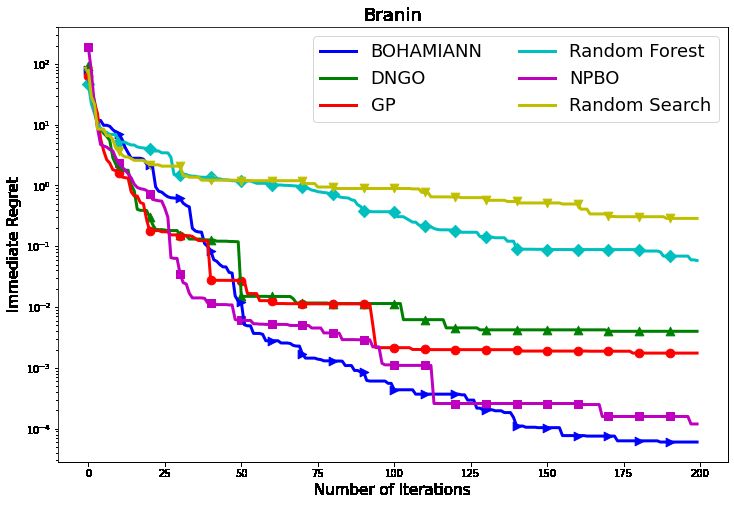
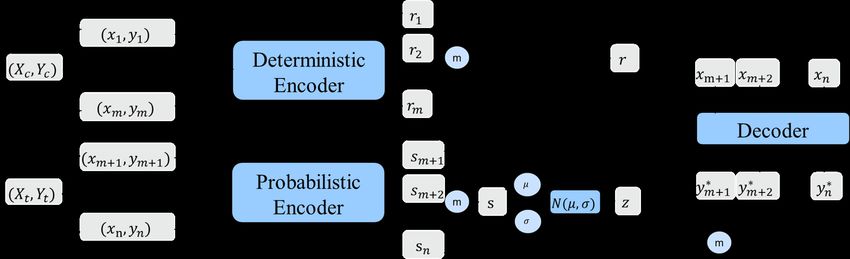
Figure 1: Flowchart of Neural Process.

the deterministic encoder to produce the global representa-                       uncertainty estimations over unknown parameters. NP also
tion of r and the target points are fed to the probabilistic en-                  combines benefits of neural networks so that is scaled lin-
coder to generate s that generates z. In this process, we as-                     early with respect to the number of observations.
sume that we only have the information of the context points,
and want to predict the target points. After this data splitting                                        Experiments
process, ELBO becomes:                                                            In this section, we compare the performance of NPBO on
  logp(Yt |Xt , Xc , Yc )                                                         a power system parameter optimization problem with ran-
                      "     n
                                                                              #
                            X                                 p(z|Xc , Yc )       dom search, GP-based Bayesian optimization, DNGO and
     ≥ Eq(z|Xt ,Yt )            logp(yi∗ |fz,r (xi )) + log                       BOHAMIANN. We further compare the NPBO with bench-
                       i=m+1
                                                              q(z|Xt , Yt )
                                                           (8)                    mark problems including GP-based Bayesian optimization,
  The final loss function is modified from the ELBO defined                       Random forest based Bayesian optimization, DNGO and
by (8). Because it is impossible to estimate the prior distri-                    BOHAMIANN on seven Bayesian optimization benchmark
bution of latent vector, i.e. p(z), so we use the posterior of                    problems.
context points q(z|Xc , Yc ) to approximate p(z|Xc , Yc ):
                                                                                  Parameter Optimization for Power System
  logp(Yt |Xt , Xc , Yc )
                      "     n
                                                                              #   Accurate and validated machine models are essential for
                            X                                 q(z|Xc , Yc )       reliable and economic power system operations. Machine
     ≥ Eq(z|Xt ,Yt )            logp(yi∗ |fz,r (xi )) + log
                       i=m+1
                                                              q(z|Xt , Yt )       models need to be regularly calibrated to ensure their ac-
                                                             (9)                  curacy for planning purpose and real-time operation (Huang
We use the lower bound of (9) as the loss function. In or-                        et al. 2017). In recent years, power generation is facing sub-
der to obtain q(z|Xc , Yc ), the context points will be fed                       stantial changes to its power grid with increasing additions
into probabilistic encoder for only the forward process. Note                     of renewable energy sources and generators. Consequently,
that (9) contains two terms. The first is the expected log-                       it is critical to the system operators to have efficient cali-
likelihood over the target points. To calculate the first term,                   bration methods and tools in order to reduce the time and
we need the context parameter r and a sample from the latent                      effort required in machine calibration. To test our proposed
space z ∼ q(z|Xt , Yt ), then feed z, r and Xt to the decoder                     NPBO method, an IEEE 14-bus system (Yk 2020) with a 14-
to get the prediction of the model performance as well as its                     parameter generator model, namely the ROUND ROTOR
uncertainty. The second term evaluates the approximate neg-                       GENERATOR MODEL (GENROU) shown in Fig.2, is sim-
ative Kullback–Leibler (KL) divergence (Joyce 2011) be-                           ulated using the power system simulation tool, PSS R E (We-
tween q(z|Xc , Yc ) and q(z|Xt , Yt ), since we replace the                       ber 2015). The simulator takes the 14-dimensional parame-
prior of z ∼ p(z) to the posterior z ∼ q(z|Xc , Yc ). In the                      ter of a generator model as the input, where their physical
inference process, we use all points observed as the context                      meanings are shown in Table 1, to generate a 4-dimensional
points, and z is generated using this context points instead of                   output measured on the bus terminal that is connected to
target points; then perform the forward step of the training                      the target generator, i.e., Bus Voltage Magnitude (voltage),
process to get the prediction which will be fed to Equ. (3) to                    Bus Voltage Frequency (frequency), Real Power Injection
determine the next point to query.                                                (P) and Reactive Power Injection (Q). To reduce the param-
   Similar to GP, NP models distributions over functions and                      eter dimension, the Design of Experiments (DOE), a well-
provides uncertainty estimations. Therefore, it is very suit-                     established statistical approach, has been applied to select
able to be applied as the surrogate model under the Bayesian                      a subset of four out of 14 parameters (Gunawan, Lau et al.
optimization framework. In other words, NP learns an im-                          2011). That is, our goal is to optimize the selected four pa-
plicit kernel from the data directly, which reduces the hu-                       rameters so that the simulated output matches the target ob-
man effort to design the kernel function in GP, and leads to                      servations. The ranges of input parameters to be optimized
Table 1: Input parameters and their physical meaning
T 0 do d-axis OC Transient time constnat
T 00 do Subtransient
T 0 qo Transient
T 00 qo Subtransient
H H Inertia
D D speed Daping
Xd Direct Axis Reactance
Xq Quadrature Axis Reactance
X 0d Direct Axis Transient Reactance
X 0q Quadrature Axis Transient Reactance
X d/X 00 q
00
Subtransient Reactance
XI Leakage Reactance
S(1.0) Saturation First Point
S(2.0) Saturation Second Point
Table 2: Input and Output range of the power system
Min Max
T 0 do 5.625 9.375
Xd 1.425 2.375
Input Figure 2: The IEEE 14 bus system.
Xq 1.35 2.25
X 0d 0.315 0.525
P −2.4612 1.8012 Table 3: Evaluation of Different Parameter Optimization
Q −0.5418 8.3188 Methods for power system
Output
f requency −8.5615 6.8365
voltage 0.9987 1.0001 Experiment Time(s) MSE
Random Search 20 2.001
GP 349 1.759 × 10⁻¹
and observations are shown in Table 2. DNGO 409 1.504 × 10⁻¹
We use Mean Square Error (MSE) of the estimated pa- DNGO(Residual) 997 1.758 × 10⁻¹
rameters to evaluate the performance: BOHAMIANN 1672 2.718 × 10⁻²
Tr XD NPBO 157 5.182 × 10⁻³
1 X
M SE = (Pij − Pˆij )2 (10)
T r × D i=1 j=1
where T r is the number of trials (e.g., each trial is initialized NPBO has the most accurate parameter calibration among
with a new set of ground-truth parameters), D is the number all the models with a very short execution time.
of parameters to be optimized, i.e., the parameter dimension, We further compare the four-dimensional outputs of the
Pij and P̂ij represent the ground-truth and estimated j th pa- power system with the optimized parameters using NPBO
to the observed target outputs in Fig. 3 . As it can be seen,
rameter in ith trial, respectively. The term ground-truth de-
there is only a very small difference between our optimized
notes to the parameter combination that generates expected
output and the target output, which indicates, with only a few
outputs. In our experiment, the objective function that needs
observations, we can still obtain accurate and satisfactory
to be minimized is defined by
parameter values.
m
X
D= ||Oi − Ôi ||2 (11) Seven Benchmark Problems
i=1
To demonstrate the effectiveness of our approach, we com-
where m = 4 is the dimension of the output, Oi and Ôi are pare NPBO to the state-of-the-art Bayesian optimization
vectors of length 452 that represent outputs of ground-truth methods using different surrogate models on a set of syn-
and of estimated parameters respectively. We set T r = 100, thetic functions (Klein et al. 2017). Besides GP-based
and in each run, we query 500 observations. The experi- Bayesian optimization, DNGO and BOHAMIANN, we also
ments are run on an Intel i7-9700k, and the results are shown use Random Forest (Hutter, Hoos, and Leyton-Brown 2011)
in Table 3. As residual block (He et al. 2016) has seen great as the surrogate model in comparison. The goal is to find
success in NNs, we re-implement a DNGO with two resid- the parameters that minimize the synthetic functions. The
ual blocks and add it for comparison. As the table shows, results based on seven benchmark problems (EggenspergerTable 4: Evaluation of Different Surrogate Models on global optimization benchmarks
Experiment Gaussian Process Random Forest DNGO BOHAMIANN NPBO
Branin 0.3996 0.4562 0.4019 0.3979 0.3980
Camelback −1.011 −0.8085 −1.026 −1.027 −0.9999
Hartmann3 −1.028 −0.998 −3.862 −3.861 −3.498
Forrester −6.021 −6.021 −5.846 −6.021 −5.301
GoldsteinPrice 4.916 27.69 6.379 11.39 8.654
Hartmann6 −3.255 −3.132 −3.249 −3.264 −3.214
SinOne 0.04292 0.06472 0.04292 0.04292 0.04292
Top-3 best algorithms for each benchmark problem are bolded.
Figure 3: Comparison of Output from Calibrated Model and
Target Output. (a): Real power injection; (b): Reactive power Figure 4: Immediate regret of different surrogate models ap-
injection; (c): Frequency; (d) Voltage. Outputs are normal- plied to Bayesian Optimization on the Branin benchmark.
ized using Min-Max Normalization method. Result averaged over 10 runs.
et al. 2013) are shown in Table 4. These benchmark prob-
lems are popular synthetic functions with the number of method. NPBO has the ability to efficiently identify the op-
parameters range from one to six, e.g., Branin and Hart- timal parameter combination of black-box models. The pro-
mann function (Surjanovic and Bingham 2013). As the ta- posed model preserves the advantage of the GP such as flex-
ble shows, all surrogate models with Bayesian optimization ibility and estimation of uncertainty, while reduces the time
achieved acceptable performance. Overall, among the seven complexity from cubic to linear and improves the accuracy
benchmark problems, NPBO performs competitive to BO- in uncertainty estimation. NPBO is applied to optimize the
HAMIANN, DNGO and GP based Bayesian optimization parameters of a complex 14-parameter generator models in
on four problems. an IEEE 14-bus power system and the results show that
We further show the optimization process of Branin in NPBO outperforms the other benchmark algorithms, i.e.,
detail in Fig. 4, where the performance is measured by im- Gaussian Process, Random Forest, Deep Neural network for
mediate regret defined by (12) Global Optimization (DNGO) and Bayesian Optimization
with Hamiltonian Monte Carlo Artificial Neural Networks
I = |fˆopt
i
− fopt | (12) (BOHAMIANN). We further compared the performance of
NPBO on seven common benchmark problems with differ-
where fˆopt
i
is the optimal observed value found in ith itera- ent surrogate models and the results show NPBO has com-
tion, and fopt represents the theoretical optimal value. As it petitive performance with benchmark approaches.
can be seen, NPBO performs competitively with BOHAMI- We consider three aspects in our future work: i) we are
ANN and GP based Bayesian optimization, and its perfor- going to apply NPBO in different scenarios, e.g., accelerat-
mance exceeds random search and Bayesian optimization ing experiments in the physical science (Ermon 2020); ii)
based on random forest. we will test the performance of variants of NP as the sur-
rogate model, such as Conditional Neural Process (Garnelo
et al. 2018a) and Attentive Neural Process (Kim et al. 2019);
Conclusions and Future Work iii) acquisition function could also be replaced by NN to
In this paper, we propose Neural Process for Bayesian Op- perform the trade-off strategy under Bayesian optimization
timization (NPBO) as a scalable parameter optimization framework.References Hebbal, A.; Brevault, L.; Balesdent, M.; Talbi, E.-G.; and
Archetti, F.; and Candelieri, A. 2019. Bayesian Optimization Melab, N. 2019. Bayesian optimization using deep Gaussian
and Data Science. Springer. processes. arXiv preprint arXiv:1905.03350 .
Bergstra, J.; and Bengio, Y. 2012. Random search for hyper- Huang, R.; Diao, R.; Li, Y.; Sanchez-Gasca, J.; Huang, Z.;
parameter optimization. The Journal of Machine Learning Thomas, B.; Etingov, P.; Kincic, S.; Wang, S.; Fan, R.; et al.
Research 13(1): 281–305. 2017. Calibrating parameters of power system stability mod-
els using advanced ensemble Kalman filter. IEEE Transac-
Cassioli, A. 2013. A Tutorial on Black–Box Optimiza- tions on Power Systems 33(3): 2895–2905.
tion. [Online]. Available: https://www.lix.polytechnique.fr/ Hutter, F.; Hoos, H. H.; and Leyton-Brown, K. 2011. Se-
∼dambrosio/blackbox material/Cassioli 1.pdf.
quential model-based optimization for general algorithm
Chen, Y.; Huang, A.; Wang, Z.; Antonoglou, I.; Schrit- configuration. In International conference on learning and
twieser, J.; Silver, D.; and de Freitas, N. 2018. Bayesian intelligent optimization, 507–523. Springer.
optimization in alphago. arXiv preprint arXiv:1812.06855 . Jaderberg, M.; Dalibard, V.; Osindero, S.; Czarnecki, W. M.;
Cheng, J. 2018. Evolutionary optimization: A review and Donahue, J.; Razavi, A.; Vinyals, O.; Green, T.; Dunning,
implementation of several algorithms. [Online]. URL https: I.; Simonyan, K.; et al. 2017. Population based training of
//www.strong.io/blog/evolutionary-optimization. Available: neural networks. arXiv preprint arXiv:1711.09846 .
https://www.strong.io/blog/evolutionary-optimization [Ac- Joyce, J. M. 2011. Kullback-Leibler Divergence, 720–722.
cessed: Jun.23, 2020]. Berlin, Heidelberg: Springer Berlin Heidelberg. ISBN 978-
Duris, J.; Kennedy, D.; Hanuka, A.; Shtalenkova, J.; Ede- 3-642-04898-2. doi:10.1007/978-3-642-04898-2 327. URL
len, A.; Baxevanis, P.; Egger, A.; Cope, T.; McIntire, M.; Er- https://doi.org/10.1007/978-3-642-04898-2 327.
mon, S.; et al. 2020. Bayesian optimization of a free-electron Kim, H.; Mnih, A.; Schwarz, J.; Garnelo, M.; Eslami, A.;
laser. Physical Review Letters 124(12): 124801. Rosenbaum, D.; Vinyals, O.; and Teh, Y. W. 2019. Attentive
Eggensperger, K.; Feurer, M.; Hutter, F.; Bergstra, J.; Snoek, neural processes. arXiv preprint arXiv:1901.05761 .
J.; Hoos, H.; and Leyton-Brown, K. 2013. Towards an em- Klein, A.; Falkner, S.; Mansur, N.; and Hutter, F. 2017.
pirical foundation for assessing bayesian optimization of hy- Robo: A flexible and robust bayesian optimization frame-
perparameters. In NIPS workshop on Bayesian Optimization work in python. In NIPS 2017 Bayesian Optimization Work-
in Theory and Practice, volume 10, 3. shop.
Ermon, S. 2020. Bayesian Optimization and Lázaro-Gredilla, M.; Quiñonero-Candela, J.; Rasmussen,
Machine Learning for Accelerating Experiments C. E.; and Figueiras-Vidal, A. R. 2010. Sparse spec-
in the Physical Sciences. [Online]. Available: trum Gaussian process regression. The Journal of Machine
https://www.youtube.com/watch?v=5n7UinKrMLk&list= Learning Research 11: 1865–1881.
PL1e3Jic2 DwwJQ528agJYMEpA0oMaDSA9&index=18. Lin, L.; Wu, W.; Shangguan, Z.; Wshah, S.; Elmoudi, R.;
Frazier, P. I. 2018. A tutorial on bayesian optimization. and Xu, B. 2020. HPT-RL: Calibrating Power System Mod-
arXiv preprint arXiv:1807.02811 . els based on Hierarchical Parameter Tuning and Reinforce-
ment Learning. In IEEE International Conference on Ma-
Garnelo, M.; Rosenbaum, D.; Maddison, C. J.; Ramalho, chine Learning and Applications.
T.; Saxton, D.; Shanahan, M.; Teh, Y. W.; Rezende, D. J.;
and Eslami, S. 2018a. Conditional neural processes. arXiv Liu, H.; Ong, Y.-S.; Shen, X.; and Cai, J. 2020. When Gaus-
preprint arXiv:1807.01613 . sian process meets big data: A review of scalable GPs. IEEE
Transactions on Neural Networks and Learning Systems .
Garnelo, M.; Schwarz, J.; Rosenbaum, D.; Viola, F.;
McIntire, M.; Ratner, D.; and Ermon, S. 2016. Sparse Gaus-
Rezende, D. J.; Eslami, S.; and Teh, Y. W. 2018b. Neural
sian Processes for Bayesian Optimization. In UAI.
processes. arXiv preprint arXiv:1807.01622 .
Muehleisen, R. T.; and Bergerson, J. 2016. Bayesian Cali-
Görtler, J.; Kehlbeck, R.; and Deussen, O. 2019. A Visual bration - What, Why And How. In INTERNATIONAL HIGH
Exploration of Gaussian Processes. Distill 4(4): e17. PERFORMANCE BUILDINGS CONFERENCE.
Gunawan, A.; Lau, H. C.; et al. 2011. Fine-tuning algorithm Rasmussen, C.; and Williams, C. 2006. Gaussian Processes
parameters using the design of experiments approach. In for Machine Learning. Adaptive Computation and Machine
International Conference on Learning and Intelligent Opti- Learning. Cambridge, MA, USA: MIT Press.
mization, 278–292. Springer.
Snelson, E.; and Ghahramani, Z. 2006. Sparse Gaussian pro-
Gustafsson, M. 2016. Antenna current optimization and op- cesses using pseudo-inputs. In Advances in neural informa-
timal design. In 2016 International Symposium on Antennas tion processing systems, 1257–1264.
and Propagation (ISAP), 132–133. IEEE. Snoek, J.; Rippel, O.; Swersky, K.; Kiros, R.; Satish, N.;
He, K.; Zhang, X.; Ren, S.; and Sun, J. 2016. Deep resid- Sundaram, N.; Patwary, M.; Prabhat, M.; and Adams, R.
ual learning for image recognition. In Proceedings of the 2015. Scalable bayesian optimization using deep neural net-
IEEE conference on computer vision and pattern recogni- works. In International conference on machine learning,
tion, 770–778. 2171–2180.Springenberg, J. T.; Klein, A.; Falkner, S.; and Hutter, F. 2016. Bayesian optimization with robust Bayesian neural networks. In Advances in neural information processing sys- tems, 4134–4142. Surjanovic, S.; and Bingham, D. 2013. Virtual library of simulation experiments: test functions and datasets. Simon Fraser University, Burnaby, BC, Canada, accessed May 13: 2015. Weber, J. 2015. Description of Machine Models GENROU, GENSAL, GENTPF and GENTPJ. [Online]. Available: https://www.powerworld.com/files/GENROU-GENSAL- GENTPF-GENTPJ.pdf. Xiao, J.-k.; Li, W.-m.; Li, W.; and Xiao, X.-r. 2015. Op- timization on black box function optimization problem. Mathematical Problems in Engineering 2015. Yang, X. 2017. Understanding the variational lower bound. Yk, B. 2020. IEEE 14 bus System. [Online]. Available: https://www.mathworks.com/matlabcentral/fileexchange/ 46067-ieee-14-bus-system. Zhang, P.; and Zhang, P. 2010. Industrial control system simulation routines. Advanced Industrial Control Technol- ogy; Elsevier: Oxford, UK 781–810.
You can also read