A stringy perspective on the coincidence problem
←
→
Page content transcription
If your browser does not render page correctly, please read the page content below
Published for SISSA by         Springer
                                                                      Received: August 6,   2021
                                                                    Revised: September 7,   2021
                                                                  Accepted: September 16,   2021
                                                                    Published: October 6,   2021

A stringy perspective on the coincidence problem

                                                                                                   JHEP10(2021)055
Francesc Cunillera and Antonio Padilla
 School of Physics and Astronomy, University of Nottingham,
 Nottingham NG7 2RD, U.K.
 E-mail: francesc.cunilleragarcia@nottingham.ac.uk,
 antonio.padilla@nottingham.ac.uk

Abstract: We argue that, for string compactifications broadly consistent with swampland
constraints, dark energy is likely to signal the beginning of the end of our universe as
we know it, perhaps even through decompactification, with possible implications for the
cosmological coincidence problem. Thanks to the scarcity (absence?) of stable de Sitter
vacua, dark energy in string theory is assumed to take the form of a quintessence field in slow
roll. As it rolls, a tower of heavy states will generically descend, triggering an apocalyptic
phase transition in the low energy cosmological dynamics after at most a few hundred
Hubble times. As a result, dark energy domination cannot continue indefinitely and there
is at least a percentage chance that we find ourselves in the first Hubble epoch. We use a
toy model of quintessence coupled to a tower of heavy states to explicitly demonstrate the
breakdown in the cosmological dynamics as the tower becomes light. This occurs through a
large number of corresponding particles being produced after a certain time, overwhelming
quintessence. We also discuss some implications for early universe inflation.

Keywords: Classical Theories of Gravity, Cosmology of Theories beyond the SM,
Superstring Vacua

ArXiv ePrint: 2105.03426

Open Access, c The Authors.
                                                     https://doi.org/10.1007/JHEP10(2021)055
Article funded by SCOAP3 .
Contents
1 Introduction 1
2 Generic idea 2
3 A toy model 5
4 Discussion 10
JHEP10(2021)055
1 Introduction
A slew of observations, from supernova [1, 2] to the cosmic microwave background [3], point
to a standard model of cosmology in which the universe was dominated by radiation at early
times, then by matter, before entering the current phase of dark energy domination. The
microscopic origin of dark energy has not been established although on cosmological scales
we know that it behaves like a fluid whose equation of state is very close to ωDE ≈ −1 [4].
This leads to a near constant energy density, consistent with a cosmological constant [5] or
a slowly rolling quintessence field [6–8]. Assuming the underlying physics is governed by
quantum field theory, the density of dark energy should be boosted by the energy of the
quantum vacuum to values far in excess of those we observe, a puzzle normally referred to
as the cosmological constant problem (for reviews see [9–12]). A related but qualitatively
distinct puzzle is the cosmological coincidence problem. This is usually presented as a
simple question: why now [13, 14]? Why do we happen to live at a time when the energy
density of matter and dark energy are roughly comparable? It is this latter problem that
we seek to discuss in this paper, in the context of string compactifications and a consistent
theory of quantum gravity.
Let us unpack the problem in a little more detail. The total age of the universe is
estimated to be around 13.7 Gyrs [3]. The early phase of radiation domination represents
only a small fraction of that history, giving way to matter after around 51 Kyrs, at a
redshift of zeq ≈ 3400. The transition to dark energy domination occurred much later,
after around 3.5 Gyrs, at a redshift of zde ≈ 0.5. This represents roughly a quarter of the
universe’s current lifetime [15]. This means that the universe has been matter dominated
for a significant fraction of its history, so much so that its density today is still comparable
to that of dark energy.
Why is this a problem? The issue is the rate at which dark energy dilutes in comparison
to matter, if indeed it dilutes at all. If dark energy is a cosmological constant, as in the
standard ΛCDM cosmology, its energy density remains constant while the energy density
of matter falls off exponentially quickly once we enter the accelerating phase. If we take the
standard scenario at face value, dark energy will dominate indefinitely. It seem implausible
that we should find ourselves so close to the dawn of dark energy domination, within a
single Hubble time. By way of comparison, we note that planetary orbits are expected to
exist for another 105 Hubble times [16].
–1–There have been several proposals that touch upon aspects of this problem (see [15]).
These range from anthropic considerations [17–20] to k-essence scenarios where dark en-
ergy is triggered by matter-radiation equality, coming to dominate within a few billion
years [21–23]. Although the latter go some way to explaining the (limited) duration of the
matter dominated epoch, they do not address the main question of why we happen to find
ourselves so close to the dawn of dark energy domination.
This particular question can be addressed in apocalyptic fashion by bringing the uni-
verse to a rapid conclusion. The basic idea is that dark energy domination begins with
acceleration before triggering cosmic Armageddon, within a few efolds. The solution to the
JHEP10(2021)055
coincidence problem follows because the accelerated epoch is cut short — it does not go on
indefinitely and endures for a similar time to matter domination. This was shown to occur
in phantom cosmologies [20, 24], linear quintessence [20, 25] and sequestering scenarios [26].
The purpose of this paper is to investigate the extent to which string theory may point to a
similar resolution of the coincidence problem via the swampland conjectures [27–31]. Our
goal is to be as generic as possible — some closely related ideas can, of course, be found
in the swampland cosmology paper [35] and in [36], in the context of the Ijjas-Steinhardt
cyclic models [37].
2 Generic idea
We begin with the distance conjecture [29, 32–34], which is one of the most well studied
and least controversial of the swampland conjectures (see also [41–48, 55]). This states
the following: consider two points in field space, φ0 and φ0 + ∆φ, separated by a geodesic
distance ∆φ. As ∆φ → ∞, there exists an infinite tower of states whose mass become
exponentially light,
|∆φ|
−β M
m(φ0 + ∆φ) ∼ m(φ0 )e Pl (2.1)
for some positive constant, β, that we typically expect to be O(1). The offending tower
of states is often associated with Kaluza-Klein modes or winding modes, depending on
the direction of motion in moduli space. For this reason, we take the initial mass m(φ0 )
to be given by the scale of compactification, 1/R, which could be as low as a few meV
in a braneworld setting where Standard Model fields are confined to a 3-brane, although
generically we expect it to be much larger, perhaps even just short of the Planck scale,
MPl ∼ 1018 GeV.
In its refined form, the de Sitter swampland conjecture [38–40] concerns the form
of the potential V (φ) for scalar fields in a low energy effective theory. Assuming the
effective theory is obtained from a consistent theory of quantum gravity, the potential
must satisfy either
c
|∇V | ≥ V (2.2)
MPl
or
c0
min (∇i ∇j V ) ≤ − 2 V (2.3)
MPl
–2–where c, c0 are universal positive constants of O(1) and min (∇i ∇j V ) is the minimum
eigenvalue of the corresponding Hessian. Note that the conjecture forbids the existence of
stable de Sitter vacua in string theory, for which we would have to have V > 0. It does,
however, allow for de Sitter vacua with a tachyonic instability of order the corresponding
√
Hubble time H −1 ∼ MPl / V . Some constraints on the scale of the tachyon were recently
derived in the context of 10D supergravity [63].
The absence of stable de Sitter vacua points towards a dynamical model of dark energy.
Of course, building a reliable model of quintessence within string theory is not without its
own challenges [62]. Nevertheless, we begin with a model of quintessence as a canoni-
cal scalar field, φ, moving under the influence of a potential V . Here we imagine that
JHEP10(2021)055
quintessence is generically described by the saxions of string theory with a non-compact
field range. The energy density and pressure stored in the field are given respectively by
ρφ = 12 φ̇2 + V and pφ = 12 φ̇2 − V . The dynamics of the scalar is governed by the following
field equation
φ̈ + 3H φ̇ + V 0 (φ) = 0 (2.4)
where H(t) is the Hubble parameter and “dot” denotes differentiation with respect to
cosmological time. Our goal is to argue that dark energy domination is relatively short
lived on account of the motion of the field towards the infinite points in moduli space.
Any motion of the field prior to dark energy domination will only reduce the amount it is
allowed to move afterwards, bringing dark energy to an even quicker conclusion. Therefore,
the most conservative scenario is to assume negligible motion of the moduli fields until dark
energy finally begins to dominate. This is, in any event, likely as the field will be held up
by Hubble friction.
Once the dark energy field has come to dominate, to be compatible with the observed
equation of state, it must be in slow roll, 12 φ̇2
V, |φ̈|
3H|φ̇|. Furthermore, we may
assume that H ≈ H0 ∼ 10−33 eV ∼ 10−60 MPl . With these approximations, consider the
field excursion in a short time δt. This is given by
V0
δφ ≈ − δt (2.5)
3H0
If we accept the refined de Sitter conjectures, then one of (2.2) or (2.3) must hold. Let’s
assume we satisfy the condition on the gradient, given by (2.2). It now follows that
c V
|δφ| & δt ∼ O(1)MPl H0 δt (2.6)
MPl 3H0
ρφ
where we have used the Friedmann equation during dark energy domination H02 ≈ 2
3MPl
≈
V
2
3MPl
and the fact that c is assumed to be O(1). We immediately see that the dark energy
field rolls roughly a Planck unit in a Hubble time. We now consider the implications for the
distance conjecture (2.1), assuming the tower of new states are initially very heavy, with
masses m(φ0 ) ∼ MPl close to the Planck scale. After a single Hubble time, the dark energy
field will move by around one Planck unit. This only corresponds to a fractional change in
the masses in the tower, and certainly not enough to contaminate the low energy physics.
–3–How far is the field allowed to roll before we have to start worrying about it? In
the local neighbourhood of the Earth the field should not be displaced from φ0 by more
than around 30 Planck units. Anything more than that would bring the mass of the
tower down from Planck scale to the scale of collider physics, opening up the possibility
of producing these states at the LHC. Of course, the details of this depend on the nature
of the coupling between the tower and the Standard Model fields. Furthermore, none
of these considerations are relevant on cosmological scales, where we can certainly allow
the field to move much further. To ensure that the tower remains decoupled from the
low scale cosmological dynamics, we conservatively impose a maximum displacement of
|∆φ|max ∼ MβPl ln(MPl /H0 ). For β ∼ O(1) this corresponds to a displacement of around
JHEP10(2021)055
140 Planck units. Assuming the field continues to roll a Planck unit in every Hubble
time, we see that the tower of states will trigger a transition in the cosmological dynamics
after no more than O(100) Hubble times. The coincidence problem isn’t solved but it is
significantly ameliorated. If a generic model of dark energy is destined to last at most
O(100) Hubble epochs, and all epochs are equally probable, we might expect there to be at
least a percentage chance that we find ourselves in the first epoch. By way of comparison,
we note that when Leicester City won the premier league in 2016, they started the season
as 5000-1 outsiders.
What if we assume that we satisfy the second of the two de Sitter swampland crite-
ria (2.3), rather than the first (2.2)? If the condition on the gradient (2.2) is violated, but
the condition on the Hessian (2.3) holds the dark energy field may move considerably less
than a Planck unit in a Hubble time. In fact, if we imagined the field sitting in a region
where the gradient of the potential is negligible, we might even imagine it staying there
indefinitely, giving a neverending period of dark energy. However, this conclusion is too
quick. Quantum fluctuations will guarantee a displacement in the field of at least O(H0 )
in the first Hubble time. This initial displacement will grow thanks to the fact that the
Hessian condition implies a tachyonic mass for the fluctuations in the dark energy field,
0
µ2 = V 00 (φ) < 0 with |µ2 | & Mc 2 V ≈ 3c0 H02 . For c0 ∼ O(1), the corresponding instability
Pl
can be as slow as a Hubble time but even so, its effect is amplified over several Hubble
times by exponential growth. There are two possibilities: the first is that the instability
triggers a rapid transition which brings the acceleration to a premature end (as desired
for the coincidence problem). This could occur, for example, by the potential changing
sign so that we no longer have a quasi de Sitter expansion. Alternatively, the background
cosmology could remain roughly unchanged, at least beyond a few Hubble times. If this is
the case, the tachyonic instability amplifies the initial displacement to a value 1
|δφ| & H0 eO(1)H0 δt (2.7)
In the latter scenario, the tower of massive states would remain decoupled from the
cosmological dynamics until |δφ| ≈ |∆φ|max ∼ MβPl ln(MPl /H0 ), at which point a transition
1
To leading order, the scalar satisfies an equation φ̈ + 3H0 φ̇ − |µ2 |φ = 0, where we recall that µ2 =
0
V (φ) < 0 with |µ2 | & Mc 2 V ≈ 3c0 H02 . The general solution is then given by a sum of exponentials eλ± t
00
√ 2 Pl 2
−3H0 ± 9H0 +4|µ |
where λ± = 2
, which includes a growing mode, with λ+ & H0 , thanks to the tachyonic
instability with |µ2 | & H02 .
–4–is inevitable. For β ∼ O(1), this will occur within at most ln[MPl /H0 ln(MPl /H0 ))] ∼ 143
Hubble times, so our conclusions are unchanged, and the coincidence problem isn’t as
serious as we previously thought.
Of course, the de Sitter conjecture is less well established than the distance conjecture,
and, in the simplest scenarios, may even be at odds with local measurements of H0 [64].
With this in mind, what can we say if we deny the validity of both criteria (2.2) and (2.3)
and abandon the de Sitter conjecture altogether? In this instance, we cannot rule out
the possibility that the current phase of acceleration is approaching a stable de Sitter
configuration in which dark energy continues for an exponentially large number of Hubble
JHEP10(2021)055
epochs. If this is the case, then the coincidence problem is as problematic as ever. However,
we might tentatively speculate that the de Sitter conjecture is really a statement about
what is generic within consistent models of dark energy within string theory. Of course,
it is much too early to make any definitive statement in this regard. Nevertheless, if it
happens to be true that the generic scenarios are those for which one of the criteria (2.2)
or (2.3) hold, our results go through and the coincidence problem is tamed. We might also
worry about the fact we have assumed dark energy to be a single canonical scalar. However,
we expect this to capture the generic dynamics of fields moving through moduli space, with
our canonical scalar tangential to the trajectory and all the orthogonal directions stabilised.
3 A toy model
To better understand how an accumulation of light states can impact the cosmological
evolution at late times, we consider a toy model of dark energy described by the following
Lagrangian
∞
1 − αφ X 1 1 −2 βφ
L = − (∂φ)2 − µ4 e MPl + − (∂ϕn )2 − n2 MKK
2
e MPl ϕ2n (3.1)
2 n=1
2 2
Here φ is the quintessence field, driving dark energy, taken to be in slow roll on a runaway
αφ
−
potential of the form µ4 e MPl where µ4 = 3Mpl 2 H 2 is the scale of dark energy and α is some
0
order one positive number. To be compatible with observations we require α < 0.6 [35],
which is not in conflict with the swampland constraints on the potential (2.2) and (2.3). In
addition we have a tower of heavy states, ϕn , whose masses are originally set by some high
scale MKK (imagined to be the Kaluza-Klein scale associated with the compact internal
manifold), becoming exponentially light as the dark energy field, φ, rolls off to infinity.
The rate at which the tower becomes light is set by the coupling β, which is also assumed
to be order one and positive.
At the dawn of dark energy domination, at time t0 , we assume that the quintessence
field is far away from the tails of the exponentials, φ ∼ φ0
MPl /α, MPl /β. Since the
βφ0
−
effective mass of the Kaluza-Klein tower, MKK e MPl ∼ MKK
H0 is high in this regime,
far above the scale of the cosmological evolution, the Kaluza-Klein states are decoupled
from the dynamics. As a result, the quintessence field satisfies the following classical
–5–equation of motion on a homogenous and isotropic background
α 4 − Mαφ
φ̈ + 3H φ̇ − µ e Pl = 0 (3.2)
MPl
For a quasi-de Sitter expansion, with H ≈ H0 , we find that φ ≈ φ0 + λ(t − t0 ) where
αµ4
λ= = αMPl H0 < MPl H0 (3.3)
3MPl H0
This approximation works well as long as ∆φ < MPl /α, or equivalently, ∆t < H0−1 /α2 .
Of course, acceleration will continue beyond this time, only at a lower scale. There is a
JHEP10(2021)055
wealth of literature on the dynamics of similar quintessence models (for a review, see [4]).
In this letter, we wish to briefly explore another effect that is far less well studied — the
time dependence on the mass of the Kaluza-Klein tower as the field begins to slowly roll.
On the quasi-de Sitter background with constant curvature, this is given by
− Mβs
eff
MKK (t) = MKK e Pl ≈ MKK e−(t−t0 ) (3.4)
where = βλ/MPl = αβH0 . This will drive particle production in the Kaluza-Klein
sector, kicking in as soon as the states stop being decoupled, MKK eff (t) . H . A complete
0
analysis of this phenomena requires a detailed numerical study of particle creation on the
dynamical background, taking into account the effect of the time varying mass and the
de Sitter cosmology. This work [50] is now underway but beyond the scope of the current
letter. To get some immediate insight into what might happen we neglect the curvature
of the background spacetime and focus on the particle production due to a mass varying
exponentially with time on a Minkowski geometry. Crucially, these approximations allow
us to make preliminary analytic estimates but we should also acknowledge their limitations.
In particular, we are implicitly assuming that the dark energy field, which feeds into the
effective mass of the Kaluza Klein tower, continues to evolve linearly in time beyond the
first Hubble epoch. In truth, the Hubble scale changes and the dark energy field picks
up additional temporal dependence which may affect some of the details. Also, we are
neglecting the effect of spacetime curvature. This is less of an issue, as our interest here is
on the effect of the changing mass of the Kaluza-Klein tower, as opposed to the effect of
quantum fields propagating on de Sitter. We also expect this approximation to accurately
capture the physics on sub-horizon scales.
With these caveats in mind, let us take a closer look at the nth state in the Kaluza-Klein
tower on a Minkowski background, whose dynamics described by the following Lagrangian
1 1
L = − (∂ϕn )2 − n2 MKK
2
e−2t ϕ2n (3.5)
2 2
where we have also set t0 = 0 (without loss of generality). Our analysis follows the standard
techniques reviewed in detail in [49], whose conventions we also follow. As explained
in [49], the state operator for the quantum field can be expanded in terms of creation and
annihilation operators, â†k and âk , in the usual way,
1 d3 k h
Z i
ϕ̂n (t, x) = √ 3 eik·x ūk (t)âk + e−ik·x uk (t)â†k (3.6)
2 (2π) 2
–6–where “bar” denote the complex conjugate. The mode functions are governed by the
equation for a time dependent harmonic oscillator
h i2
ük + ωk2 (t)uk = 0, ωk2 (t) = k 2 + n2 MKK
eff
(t) (3.7)
and have solutions that are conveniently expressed in terms of Hankel functions (of the
first kind)
(1) (1)
uk (t) = AHiµ (z) + B H̄iµ (z) (3.8)
where z = nMKK e−t and µ = k . Since [MKK
eff (t)]2 > 0, at any given time t we can define
∗
the instantaneous vacuum state |0i∗ as the lowest energy state of the Hamiltonian at that
JHEP10(2021)055
time. The mode functions that determine this state satisfy the boundary condition [49]
1 q
uk (t∗ ) = p , u̇k (t∗ ) = i ωk (t∗ ) (3.9)
ωk (t∗ )
This fixes the constants in (3.8) so that
πie−πµ ωk (t∗ ) (1)
(1)
A= p z∗ H̄iµ 0 (z∗ ) + iH̄iµ (z∗ ) (3.10)
4 ωk (t∗ )
πie−πµ ωk (t∗ ) (1)
(1) 0
B=− p z∗ Hiµ (z∗ ) + iHiµ (z∗ ) (3.11)
4 ωk (t∗ )
The mode functions that determine the “in” vacuum at the beginning of the dark energy
era, uin
k (t), are given by these expressions for A, B with the choice t∗ = 0. The mode
functions uout
k (t), that determine the “out” vacuum at some later time, T , are given by
the same formulae but with t∗ = T . As usual, the two can be related by a Bogoliubov
transformation, of the form uin out out
k (t) = αk (T )uk (t) + βk (T )ūk (t). At time T > 0, the true
vacuum state differs from the initial vacuum state, and so the latter contains particles.
As explained in [49], the mean particle number density for modes of momentum k is
Nk (T ) = |βk (T )|2 with corresponding energy density Ek (T ) = ωk (T )Nk (T ). When we
calculate this explicitly, it turns out that
π 2 −2πµ 2 h 2 i
Nk (T ) = e X +Y2 (3.12)
16
where
(1) (1) (1) (1)
zin Hiµ 0 (zin ) zout H̄iµ 0 (zout )
p p
ωk (0)Hiµ (zin ) ωk (T )H̄iµ (zout )
X = Im p p − (3.13)
ωk (0) ωk (T )
and
(1) (1) (1) (1)
zin Hiµ 0 (zin ) ωk (0)H̄iµ (zin ) zout H̄iµ 0 (zout )
p p
ωk (T )H̄iµ (zout )
Y = Im p − p (3.14)
ωk (0) ωk (T )
Here zin = nMKK and zout = nMKK e−T . We can obtain estimates for the energies stored in
different momentum modes by using the approximations for Bessel and Hankel functions
–7–JHEP10(2021)055
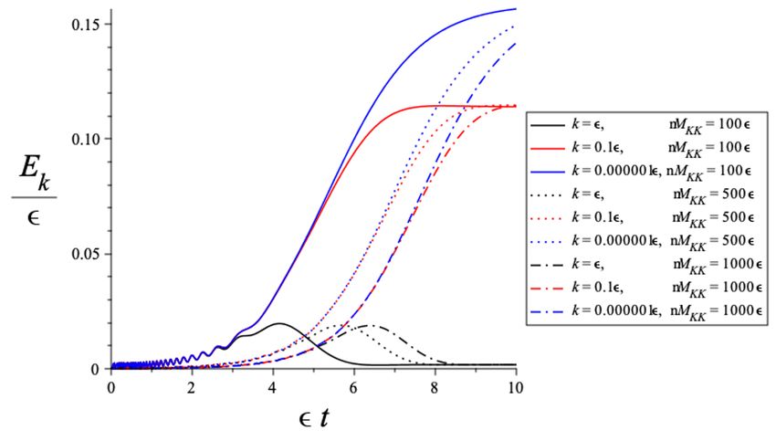
Figure 1. Plot of energy versus time for a range of scalar modes of different momentum and
different values for the initial mass. These particular plots were produced using Maple 2020 and a
numerical value of = 0.01.
given in [51]. In particular, we note that for large z
µ2 + 1, we have the following
asymptotic expansion
" #
4µ2 + 1
r
(1) 2 µπ +i(z− π )
Hiµ (z) ≈ e2 4 1+ + ... (3.15)
πz 8iz
(1)
To obtain an approximation in the opposite limit, for small z, we recall that Hiµ (z) =
eµπ Jiµ (z)−J−iµ (z)
sinh µπ and use the fact that
z " #
eiµ ln 2 z2 z4
Jiµ (z) ≈ 1− + + ... (3.16)
Γ(1 + iµ) 4(1 + iµ) 32(1 + iµ)iµ
p
whenever 0 < z
|µ| + 1.
For high momentum modes, with k → ∞, we find that
n4 MKK
4 2 h i
Ek ∼ cosh 2
t − cos 2
kt e−2t .
4k 5
As expected, these modes are suppressed, being insensitive to the change in the mass of
the field. For modes of lower momentum, it is instructive to display the changes in the
energy stored in each mode in a characteristic plot, such as the one shown in figure 1. The
plot shows the energy profile for modes running over a range of different momenta. We
also vary over the initial mass of the scalar, nMKK , or equivalently, over the level in the
Kaluza-Klein tower. For the ϕn particles, at level n, we see that the total energy density at
late times is dominated by modes
of momentum k . , with significant particle production
1 nMKK
kicking in at a time tn ∼ ln . Using (3.15) and (3.16), we can estimate the energy
–8–stored in the low energy modes analytically, for t
tn . Since nMKK e−t
nMKK
and k . , we have zout
1
zin and µ . 1, so that the energies approximate as
kπ
ke−
Ek ≈ (3.17)
kπ
2 sinh
In deriving this, we have used the relation |Γ(iµ)|2 = π/µ sinh µπ, which follows from
Euler’s reflection formula and the fact that Γ(−iµ) = Γ(iµ). To obtain an estimate for the
total energy density stored in ϕn particles at late times (t
tn ), we simply integrate this
result over all momentum. The result is
π
Z
JHEP10(2021)055
ρn = d3 kEk ≈ 4 (3.18)
60
By itself, this would only have a tiny effect on the cosmological background, since 4 =
(αβ)4 H04 , far below the scale of the critical density of the universe during the dark energy
era, MPl2 H 2 . Of course, the formula will receive additional corrections from the fact that
0
the fields are actually propagating on a dynamical cosmological background, as opposed
to Minkowski, although these are likely to be similarly suppressed,
especially if αβ & 1.
Nevertheless, by the time we have reached time tN ∼ 1 ln N MKK for some large N , we
have started to produce particles for each of the first N levels in the Kaluza-Klein tower.
The total energy density of all these particles, in this approximation, is given by
N
X Nπ 4
ρtotal (t ∼ tN ) = ρn ≈ (3.19)
n=1
60
M2
This will start to affect the cosmological dynamics for N ∼ Ncrit where Ncrit ∼ 2Pl , at a
time tcrit ∼ 1 ln Ncrit MKK . If we assume αβ ∼ O(1), then ∼ H0 and so Ncrit ∼ 10120 .
√
Assuming MKK . MPl , so that Ncrit
Ncrit & MKK , we see that tcrit . O(400)/H0 ,
confirming our expectation that the dark energy era will not last beyond a few hundred
or so Hubble times, before the space begins to decompactify. If we lower the underlying
Kaluza-Klein scale, MKK , or consider models with αβ > 1, the dark energy era is cut short
even earlier.
By the time dark energy succumbs to the extra dimensions, a huge number of particles
species have already entered the low energy effective theory. We might be worried that
this creates a “species problem” at some earlier time, lowering the scale at which gravity
becomes strongly coupled. However, for N < Ncrit species, the scale of strong coupling
√
scales as ΛQG ∼ MPl / N > H0 . In other words, four-dimensional gravity does not
become strongly coupled on cosmological scales prior to tcrit , at which point the effective
four-dimensional description breaks down anyway.
As emphasized earlier, everything we are saying is only relevant to cosmological dy-
namics. On shorter scales, for example in the lab or in the solar system, the quintessence
field may be displaced from its cosmological value, so much so that the Kaluza-Klein tower
remains heavy and decoupled from the low energy physics. Indeed, if quintessence is cou-
pled to matter with gravitational strength, such a displacement is likely to be necessary in
order to avoid fifth force constraints [52–54]. It would certainly be interesting to investigate
the implications of this in more detail.
–9–4 Discussion
In this paper, we have argued that string theory compactifications consistent with swamp-
land constraints automatically prevent the dark energy era from extending beyond a few
hundred Hubble times. This alleviates the coincidence problem to some degree, inasmuch
as we now have as much as a percentage chance of finding ourselves in the first e-fold of
acceleration. Our conclusions draw on two key features of string compactifications: (i) the
scarcity (absence?) of stable de Sitter vacua, suggesting that most dark energy models will
be driven by a quintessence field in slow roll [38, 40]; (ii) the accumulation of a large num-
ber light states as the field rolls off towards infinity [29, 32–34]. Generically, the dynamics
JHEP10(2021)055
is such that the descending tower of light states induces a cosmological phase transition,
bringing the dark energy era to a conclusion. We were able to demonstrate this explicitly
with a toy model, whereby particle creation in the Kaluza-Klein sector starts to overwhelm
the cosmological background within a few hundred Hubble times. This suggests we might
even think of dark energy as opening the door to the decompactification of spacetime!
From this stringy perspective, it seems that the cosmological coincidence is readily
reduced to one part in O(100) but can we do any better? Can we exploit the distance
conjecture to bring the odds even further in? One speculative possibility is to consider
dark energy a consequence of clockwork dynamics [56]. The clockwork construction allows
for the existence of a naturally light dark energy field, in a theory with uniquely high scale
couplings. But the set-up is brittle. After the dark energy field has moved just a single
Planck unit, we could imagine a tower of states contaminating the high scale physics and
the spoiling the clockwork dynamics. Without the clockwork, the dark energy dynamics
should also be spoilt. Whilst this idea is appealing we have not been able to identify
a stringy realisation of the clockwork dark energy model, at least within the context of
perturbative type IIA and IIB supergravity [57].
Finally, it is natural to ask what would happen if we applied the same analysis to early
universe inflation at a much higher scale than quintessence. Because the Kaluza-Klein
tower does not need to descend as far to contaminate the inflationary background, the
inflaton excursion is limited to just a few Planck units. As a result, we would conclude
that, generically, inflation should not extend beyond a few efolds. This seems problematic
since inflation must last for at least 50 efolds in order to address the horizon problem. Of
course, these concerns aren’t new — it is well known that early universe inflation is in some
tension with the swampland constraints [35].
An alternative approach could be to consider the axions as inflaton candidates, as
opposed to the saxions described above. However, these models are also in tension with
the swampland programme and in particular with the axionic weak gravity conjecture
(aWGC) [28]. The aWGC implies the existence of at least one instanton coupling elec-
trically to an axion such that f × Sint . MPl , where f is the axion decay constant and
Sinst is the instanton action. If the instanton couples to the inflaton, which requires a
super-Planckian field range, Sinst < 1 and we lose parametric control of the low-energy
theory. We can get around this by assuming the existence of heavy spectator axions that
do not contribute to the inflationary dynamics and that satisfy the aWGC bound. How-
– 10 –ever, stronger forms of the aWGC claim that spectator axions are not enough, imposing
further hurdles on axion inflation models which remain unsolved [58–61].
Clearly inflation presents a different challenge to the string model builders than
quintessence. However, we can tentatively speculate that aspects of the swampland pro-
gramme, and the de Sitter conjecture in particular, may conservatively be taken as an
indication of what to expect from a generic model of a scalar field in string theory, as
opposed to a hard and fast rule. With this perspective, inflation would be cut short in
a generic model, but there may be rare models allowing for many more efoldings. With
anthropic reasoning, we can then argue that it was necessary for our universe to explore
JHEP10(2021)055
these rare models in order to grow large. For quintessence, the story is different. We cannot
make the same anthropic arguments in favour of a rare model of quintessence that is long
lived, so we are drawn instead to scenarios satisfying the constraints (2.2) and (2.3). If
quintessence scenarios satisfying these constraints can be found they will imply that the
future of our universe should not last for more than a hundred or so Hubble times.
Acknowledgments
A.P. is funded by an STFC Consolidated Grant and F.C. by a University of Nottingham
studentship. We would like to thank Michele Cicoli and Francisco G. Pedro for invaluable
discussions.
Open Access. This article is distributed under the terms of the Creative Commons
Attribution License (CC-BY 4.0), which permits any use, distribution and reproduction in
any medium, provided the original author(s) and source are credited.
References
[1] Supernova Cosmology Project collaboration, Measurements of Ω and Λ from 42 high
redshift supernovae, Astrophys. J. 517 (1999) 565 [astro-ph/9812133] [INSPIRE].
[2] Supernova Search Team collaboration, Observational evidence from supernovae for an
accelerating universe and a cosmological constant, Astron. J. 116 (1998) 1009
[astro-ph/9805201] [INSPIRE].
[3] Planck collaboration, Planck 2018 results. VI. Cosmological parameters, Astron. Astrophys.
641 (2020) A6 [Erratum ibid. 652 (2021) C4] [arXiv:1807.06209] [INSPIRE].
[4] E.J. Copeland, M. Sami and S. Tsujikawa, Dynamics of dark energy, Int. J. Mod. Phys. D
15 (2006) 1753 [hep-th/0603057] [INSPIRE].
[5] W. de Sitter, Einstein’s theory of gravitation and its astronomical consequences, Third Paper,
Mon. Not. Roy. Astron. Soc. 78 (1917) 3 [INSPIRE].
[6] P.J.E. Peebles and B. Ratra, Cosmology with a Time Variable Cosmological Constant,
Astrophys. J. Lett. 325 (1988) L17 [INSPIRE].
[7] B. Ratra and P.J.E. Peebles, Cosmological Consequences of a Rolling Homogeneous Scalar
Field, Phys. Rev. D 37 (1988) 3406 [INSPIRE].
– 11 –[8] R.R. Caldwell, R. Dave and P.J. Steinhardt, Cosmological imprint of an energy component
with general equation of state, Phys. Rev. Lett. 80 (1998) 1582 [astro-ph/9708069]
[INSPIRE].
[9] S. Weinberg, The Cosmological Constant Problem, Rev. Mod. Phys. 61 (1989) 1 [INSPIRE].
[10] J. Polchinski, The Cosmological Constant and the String Landscape, in 23rd Solvay
Conference in Physics: The Quantum Structure of Space and Time, pp. 216–236 (2006)
[hep-th/0603249] [INSPIRE].
[11] C.P. Burgess, The Cosmological Constant Problem: Why it’s hard to get Dark Energy from
Micro-physics, in 100e Ecole d’Ete de Physique: Post-Planck Cosmology, pp. 149–197 (2015)
JHEP10(2021)055
[DOI] [arXiv:1309.4133] [INSPIRE].
[12] A. Padilla, Lectures on the Cosmological Constant Problem, arXiv:1502.05296 [INSPIRE].
[13] P.J. Steinhardt, Critical Problems in Physics, V.L. Fitch and R. Marlow eds., Princeton
University Press, Princeton (1997).
[14] I. Zlatev, L.-M. Wang and P.J. Steinhardt, Quintessence, cosmic coincidence, and the
cosmological constant, Phys. Rev. Lett. 82 (1999) 896 [astro-ph/9807002] [INSPIRE].
[15] H.E.S. Velten, R.F. vom Marttens and W. Zimdahl, Aspects of the cosmological “coincidence
problem”, Eur. Phys. J. C 74 (2014) 3160 [arXiv:1410.2509] [INSPIRE].
[16] F.C. Adams and G. Laughlin, A Dying universe: The Long term fate and evolution of
astrophysical objects, Rev. Mod. Phys. 69 (1997) 337 [astro-ph/9701131] [INSPIRE].
[17] J. Garriga, M. Livio and A. Vilenkin, The Cosmological constant and the time of its
dominance, Phys. Rev. D 61 (2000) 023503 [astro-ph/9906210] [INSPIRE].
[18] S. Weinberg, The Cosmological constant problems, in 4th International Symposium on
Sources and Detection of Dark Matter in the Universe (DM 2000), pp. 18–26 (2000)
[astro-ph/0005265] [INSPIRE].
[19] S.A. Bludman, Vacuum energy: If not now, then when?, Nucl. Phys. A 663 (2000) 865
[astro-ph/9907168] [INSPIRE].
[20] A. Barreira and P.P. Avelino, Anthropic versus cosmological solutions to the coincidence
problem, Phys. Rev. D 83 (2011) 103001 [arXiv:1103.2401] [INSPIRE].
[21] C. Armendariz-Picon, V.F. Mukhanov and P.J. Steinhardt, A Dynamical solution to the
problem of a small cosmological constant and late time cosmic acceleration, Phys. Rev. Lett.
85 (2000) 4438 [astro-ph/0004134] [INSPIRE].
[22] C. Armendariz-Picon, V.F. Mukhanov and P.J. Steinhardt, Essentials of k essence, Phys.
Rev. D 63 (2001) 103510 [astro-ph/0006373] [INSPIRE].
[23] M. Malquarti, E.J. Copeland and A.R. Liddle, K-essence and the coincidence problem, Phys.
Rev. D 68 (2003) 023512 [astro-ph/0304277] [INSPIRE].
[24] R.J. Scherrer, Phantom dark energy, cosmic doomsday, and the coincidence problem, Phys.
Rev. D 71 (2005) 063519 [astro-ph/0410508] [INSPIRE].
[25] P.P. Avelino, The Coincidence problem in linear dark energy models, Phys. Lett. B 611
(2005) 15 [astro-ph/0411033] [INSPIRE].
[26] N. Kaloper and A. Padilla, Sequestration of Vacuum Energy and the End of the Universe,
Phys. Rev. Lett. 114 (2015) 101302 [arXiv:1409.7073] [INSPIRE].
– 12 –[27] C. Vafa, The String landscape and the swampland, hep-th/0509212 [INSPIRE].
[28] N. Arkani-Hamed, L. Motl, A. Nicolis and C. Vafa, The String landscape, black holes and
gravity as the weakest force, JHEP 06 (2007) 060 [hep-th/0601001] [INSPIRE].
[29] H. Ooguri and C. Vafa, On the Geometry of the String Landscape and the Swampland, Nucl.
Phys. B 766 (2007) 21 [hep-th/0605264] [INSPIRE].
[30] E. Palti, The Swampland: Introduction and Review, Fortsch. Phys. 67 (2019) 1900037
[arXiv:1903.06239] [INSPIRE].
[31] T.D. Brennan, F. Carta and C. Vafa, The String Landscape, the Swampland, and the Missing
Corner, PoS TASI2017 (2017) 015 [arXiv:1711.00864] [INSPIRE].
JHEP10(2021)055
[32] D. Klaewer and E. Palti, Super-Planckian Spatial Field Variations and Quantum Gravity,
JHEP 01 (2017) 088 [arXiv:1610.00010] [INSPIRE].
[33] T.W. Grimm, E. Palti and I. Valenzuela, Infinite Distances in Field Space and Massless
Towers of States, JHEP 08 (2018) 143 [arXiv:1802.08264] [INSPIRE].
[34] R. Blumenhagen, D. Kläwer, L. Schlechter and F. Wolf, The Refined Swampland Distance
Conjecture in Calabi-Yau Moduli Spaces, JHEP 06 (2018) 052 [arXiv:1803.04989]
[INSPIRE].
[35] P. Agrawal, G. Obied, P.J. Steinhardt and C. Vafa, On the Cosmological Implications of the
String Swampland, Phys. Lett. B 784 (2018) 271 [arXiv:1806.09718] [INSPIRE].
[36] R.J. Scherrer, The Coincidence Problem and the Swampland Conjectures in the
Ijjas-Steinhardt Cyclic Model of the Universe, Phys. Lett. B 798 (2019) 134981
[arXiv:1907.11293] [INSPIRE].
[37] A. Ijjas and P.J. Steinhardt, A new kind of cyclic universe, Phys. Lett. B 795 (2019) 666
[arXiv:1904.08022] [INSPIRE].
[38] G. Obied, H. Ooguri, L. Spodyneiko and C. Vafa, de Sitter Space and the Swampland,
arXiv:1806.08362 [INSPIRE].
[39] S.K. Garg and C. Krishnan, Bounds on Slow Roll and the de Sitter Swampland, JHEP 11
(2019) 075 [arXiv:1807.05193] [INSPIRE].
[40] H. Ooguri, E. Palti, G. Shiu and C. Vafa, Distance and de Sitter Conjectures on the
Swampland, Phys. Lett. B 788 (2019) 180 [arXiv:1810.05506] [INSPIRE].
[41] F. Baume and E. Palti, Backreacted Axion Field Ranges in String Theory, JHEP 08 (2016)
043 [arXiv:1602.06517] [INSPIRE].
[42] A. Hebecker, P. Henkenjohann and L.T. Witkowski, Flat Monodromies and a Moduli Space
Size Conjecture, JHEP 12 (2017) 033 [arXiv:1708.06761] [INSPIRE].
[43] M. Cicoli, D. Ciupke, C. Mayrhofer and P. Shukla, A Geometrical Upper Bound on the
Inflaton Range, JHEP 05 (2018) 001 [arXiv:1801.05434] [INSPIRE].
[44] R. Blumenhagen, I. Valenzuela and F. Wolf, The Swampland Conjecture and F-term Axion
Monodromy Inflation, JHEP 07 (2017) 145 [arXiv:1703.05776] [INSPIRE].
[45] B. Heidenreich, M. Reece and T. Rudelius, Emergence of Weak Coupling at Large Distance
in Quantum Gravity, Phys. Rev. Lett. 121 (2018) 051601 [arXiv:1802.08698] [INSPIRE].
[46] A. Landete and G. Shiu, Mass Hierarchies and Dynamical Field Range, Phys. Rev. D 98
(2018) 066012 [arXiv:1806.01874] [INSPIRE].
– 13 –[47] S.-J. Lee, W. Lerche and T. Weigand, Tensionless Strings and the Weak Gravity Conjecture,
JHEP 10 (2018) 164 [arXiv:1808.05958] [INSPIRE].
[48] R. Blumenhagen, Large Field Inflation/Quintessence and the Refined Swampland Distance
Conjecture, PoS CORFU2017 (2018) 175 [arXiv:1804.10504] [INSPIRE].
[49] V. Mukhanov and S. Winitzki, Introduction to quantum effects in gravity, Cambridge
University Press (2007) [INSPIRE].
[50] F. Cunillera and A. Padilla, in preparation.
[51] M. Abramowitz and I. Stegun, Handbook of Mathematical Functions with Formulas, Graphs,
and Mathematical Tables, National Bureau of Standards, Applied Mathematics Series 55
JHEP10(2021)055
(1964).
[52] J. Khoury and A. Weltman, Chameleon fields: Awaiting surprises for tests of gravity in
space, Phys. Rev. Lett. 93 (2004) 171104 [astro-ph/0309300] [INSPIRE].
[53] J. Khoury and A. Weltman, Chameleon cosmology, Phys. Rev. D 69 (2004) 044026
[astro-ph/0309411] [INSPIRE].
[54] A. Padilla, E. Platts, D. Stefanyszyn, A. Walters, A. Weltman and T. Wilson, How to Avoid
a Swift Kick in the Chameleons, JCAP 03 (2016) 058 [arXiv:1511.05761] [INSPIRE].
[55] A. Font, A. Herráez and L.E. Ibáñez, The Swampland Distance Conjecture and Towers of
Tensionless Branes, JHEP 08 (2019) 044 [arXiv:1904.05379] [INSPIRE].
[56] L. Bordin, F. Cunillera, A. Lehébel and A. Padilla, A natural theory of dark energy, Phys.
Rev. D 101 (2020) 085012 [arXiv:1912.04905] [INSPIRE].
[57] F. Cunillera and A. Padilla, in preparation.
[58] J. Brown, W. Cottrell, G. Shiu and P. Soler, Fencing in the Swampland: Quantum Gravity
Constraints on Large Field Inflation, JHEP 10 (2015) 023 [arXiv:1503.04783] [INSPIRE].
[59] J. Brown, W. Cottrell, G. Shiu and P. Soler, On Axionic Field Ranges, Loopholes and the
Weak Gravity Conjecture, JHEP 04 (2016) 017 [arXiv:1504.00659] [INSPIRE].
[60] T. Rudelius, Constraints on Axion Inflation from the Weak Gravity Conjecture, JCAP 09
(2015) 020 [arXiv:1503.00795] [INSPIRE].
[61] S. Andriolo, T.-C. Huang, T. Noumi, H. Ooguri and G. Shiu, Duality and axionic weak
gravity, Phys. Rev. D 102 (2020) 046008 [arXiv:2004.13721] [INSPIRE].
[62] A. Hebecker, T. Skrzypek and M. Wittner, The F -term Problem and other Challenges of
Stringy Quintessence, JHEP 11 (2019) 134 [arXiv:1909.08625] [INSPIRE].
[63] D. Andriot, Tachyonic de Sitter solutions of 10d type-II supergravities, arXiv:2101.06251
[INSPIRE].
[64] A. Banerjee, H. Cai, L. Heisenberg, E.Ó. Colgáin, M.M. Sheikh-Jabbari and T. Yang, Hubble
sinks in the low-redshift swampland, Phys. Rev. D 103 (2021) L081305 [arXiv:2006.00244]
[INSPIRE].
– 14 –You can also read