Active Labour Market Policies for the Long-Term Unemployed: New Evidence from Causal Machine Learning - DISCUSSION PAPER SERIES

DISCUSSION PAPER SERIES

IZA DP No. 14486

Active Labour Market Policies for the
Long-Term Unemployed:
New Evidence from Causal Machine
Learning
Daniel Goller
Tamara Harrer
Michael Lechner
Joachim Wolff

JUNE 2021

DISCUSSION PAPER SERIES

IZA DP No. 14486

Active Labour Market Policies for the
Long-Term Unemployed:
New Evidence from Causal Machine
Learning
Daniel Goller Michael Lechner
University of St. Gallen University of St. Gallen and IZA
and University of Bern
 Joachim Wolff
Tamara Harrer Institute for Employment Research,
Institute for Employment Research, Nuremberg
Nuremberg

JUNE 2021

Any opinions expressed in this paper are those of the author(s) and not those of IZA. Research published in this series may
include views on policy, but IZA takes no institutional policy positions. The IZA research network is committed to the IZA
Guiding Principles of Research Integrity.
The IZA Institute of Labor Economics is an independent economic research institute that conducts research in labor economics
and offers evidence-based policy advice on labor market issues. Supported by the Deutsche Post Foundation, IZA runs the
world’s largest network of economists, whose research aims to provide answers to the global labor market challenges of our
time. Our key objective is to build bridges between academic research, policymakers and society.
IZA Discussion Papers often represent preliminary work and are circulated to encourage discussion. Citation of such a paper
should account for its provisional character. A revised version may be available directly from the author.

 IZA – Institute of Labor Economics
Schaumburg-Lippe-Straße 5–9 Phone: +49-228-3894-0
53113 Bonn, Germany Email: publications@iza.org www.iza.org

IZA DP No. 14486 JUNE 2021

 ABSTRACT
 Active Labour Market Policies for the
 Long-Term Unemployed:
 New Evidence from Causal Machine
 Learning*
 We investigate the effectiveness of three different job-search and training programmes
 for German long-term unemployed persons. On the basis of an extensive administrative
 data set, we evaluated the effects of those programmes on various levels of aggregation
 using Causal Machine Learning. We found participants to benefit from the investigated
 programmes with placement services to be most effective. Effects are realised quickly and
 are long-lasting for any programme. While the effects are rather homogenous for men, we
 found differential effects for women in various characteristics. Women benefit in particular
 when local labour market conditions improve. Regarding the allocation mechanism of
 the unemployed to the different programmes, we found the observed allocation to be as
 effective as a random allocation. Therefore, we propose data-driven rules for the allocation
 of the unemployed to the respective labour market programmes that would improve the
 status-quo.

 JEL Classification: J08, J68
 Keywords: policy evaluation, Modified Causal Forest (MCF), active labour
 market programmes, conditional average treatment effect
 (CATE)

 Corresponding author:
 Daniel Goller
 Centre for Research in Economics of Education
 University of Bern
 Schanzeneckstrasse 1
 CH-3001 Bern
 Switzerland
 E-mail: Daniel.Goller@vwi.unibe.ch

 * Michael Lechner is also affiliated with CEPR, London, CESIfo, Munich, IAB, Nuremberg, and RWI, Essen. Joachim
 Wolff is also affiliated with the Ludwig-Maximilian University, Munich, and LASER, Nuremberg. Support of the
 Swiss Science Foundation (grant SNST 407540_166999) and of the IAB under grant for the project “Estimating
 heterogeneous effects of the schemes for activation and integration on welfare recipients’ outcomes: Enhanced
 analyses by the application of machine learning algorithms” is gratefully acknowledged. A previous version of the
 paper was presented at the Causal Machine Learning Workshop, 2020, St. Gallen. We thank the participants for their
 helpful comments and suggestions. The usual disclaimer applies.

1 Introduction
 Bringing means-tested benefit recipients back to work is among the hardest tasks for

employment agencies. Still, it is of high interest for all, the society, the state, and most

importantly for the unemployed, to increase their chances to find decent jobs and leave long-

term unemployment. The classical approach of employment agencies in industrialised countries

is to provide active labour market programmes (ALMP), such as job-search and training

programmes, to selected unemployed individuals. It is therefore of great interest to labour

market authorities to understand whether those ALMP are beneficial for the long-term

unemployed and to understand which programme works best and for which types of

unemployed persons. Furthermore, a key issue is to learn how to allocate the programmes

efficiently.

 This study shares the interest of policy makers in gaining a better understanding of the

employment agencies’ tools by evaluating the existing ALMP and finding ways to improve the

counselling process and allocation of ALMP. Previous empirical evaluation of labour market

programmes focused on specific questions or investigated the effectiveness of the job-search,

training, and other programmes for a small number of different participant groups and/or

programme types (e.g., Bernhard and Kopf (2014), Hohmeyer (2012), Kopf (2013)). Those

more general findings are of interest; however, there is still a huge potential for analysing the

effects on more granular levels, and subsequently for allocating participants of training

programmes in a more individualised way.

 While estimating average effects for a population is well established in the

microeconometric literature, systematically investigating treatment effect heterogeneities is a

more challenging task. The recent, steadily growing literature on causal machine learning,

which combines the predictive accuracy in statistical learning tools (see Hastie, Tibshirani, and

 1

Friedman (2009) for an overview) and causal principles that have been known for years, offers

promising solutions to these challenges.

 Several approaches are proposed in the literature to modify machine learning tools in such

a way that they become useful for causal inference (for overviews, see e.g., Athey (2018), Athey

and Imbens (2019)). In an extensive empirical simulation study, Knaus, Lechner, and

Strittmatter (2021) evaluated many of those methods and found forest-type estimators (e.g.,

Wager and Athey (2018), Athey, Tibshirani, and Wager (2019)) to perform well in many

situations. In this study, we use the Modified Causal Forest (MCF) subsequently proposed by

Lechner (2018), since it enables us to investigate multiple treatments and systematic effect

heterogeneities on different levels of aggregation within one estimation approach. 1

 The literature on active labour market policy evaluation is substantial (e.g., the meta

studies of Card, Kluve, and Weber (2010), Card, Kluve, and Weber (2018) and Kluve (2010)

or less recent surveys on ALMP evaluation of Heckman, LaLonde, Smith (1999) as well as

Martin and Grubb (2001)). Usually, the focus is on estimating average effects for broader

populations, i.e., the average treatment effect (ATE) or the average treatment effect on the

treated (ATET). However, there is less evidence for smaller, more homogeneous and diverse

groups. This study is among the early papers in policy evaluation to systematically analyse

treatment effect heterogeneity using causal machine learning (CML) methods. In a LASSO-

based approach to analyse heterogeneous treatment effects, Knaus, Lechner, and Strittmatter

(2020) evaluate a job-search programme in Switzerland. Using administrative data from 2003,

they find heterogeneity in the short run, but effects become more homogeneous in the long run.

Knaus (2020) uses the same data and applies double machine learning methods (cf.

Chernozhukov et al. (2018)). In his analysis of training and job-search programmes in a multiple

treatment setting, he finds substantial effect heterogeneity by gender and previous labour

1
 While the estimation in this paper have been conducted with the Gauss version of the estimator, a Python version of it can be
 downloaded from PyPy.
 2

market success. In an application to a temporary public works programme, Bertrand, Crépon,

Marguerie, and Premand (2017) use data from randomised controlled trials to analyse treatment

effect heterogeneity. Using a causal forest algorithm (cf. Wager and Athey (2018)), they find

differential effects during the lock-in period. The same method is also used in an RCT

application to summer jobs in Davis and Heller (2017) and Davis and Heller (2020).

 The study most similar to ours is the work of Cockx, Lechner, and Bollens (2019)

investigating heterogeneity in employment effects of Flemish training programmes. In their

work, they use the MCF to investigate multiple training programmes, providing treatment

effects on various levels of aggregation. Especially, they find important heterogeneities

associated to language, migration status, and employability.

 A special feature of our study is that we observe the universe of job-search and training

programme participants among German means-tested benefit recipients. Having a broad range

of administrative data for over 300,000 mainly long-term unemployed individuals, we

investigate three different ALMP, namely job-training, reducing impediments, and a placement

service, with participation starting in the first quarter of 2010. For those three ALMP, the

unconfoundedness assumption needed for identification is credible as these administrative data

are available, for which we provide additional evidence in a placebo test. For a fourth

programme, in-firm training, the placebo exercise rejects the unconfoundedness hypothesis.

This programme is therefore excluded from the analysis.

 When the programmes that we analyse were introduced in 2009, the German government

attempted to create schemes that allow the job centres considerable leeway in the programme’s

design to meet the individual needs of participants. In turn, participation should positively

influence the employment perspectives of most participants. It is therefore important that we

analyse the heterogeneity of participation effects and estimate Individualised Average

Treatment Effects (IATEs). In fact, we primarily find that all investigated training and job-

 3

search programmes lead to positive employment effects for the participants. This can be found

not only on average, but most of the individuals are likely to realise additional days in regular

(i.e., unsubsidised contributory) employment if participating.

 Average results for women range from 26 to 54 more days in employment in three years

after starting the participation in the respective programmes; for men the effect is in the range

of 35 - 45 more days in regular employment. Effects emerge quickly and are long-lasting. While

placement service is the programme with the highest effects, we find substantial effect

heterogeneity. In general, those individuals with a worse labour market history benefit more

than those with a better record. For women, the place of residence and local labour market

conditions are decisive. Those located in regions with better local labour market conditions

benefit substantially more from participating in the job-search and training programmes than

those women living in areas with worse labour market conditions.

 With regard to the allocation mechanism in place, we find a random allocation to perform

equally well. While effect-based black-box allocation approaches lead to 14% higher effects

for the reallocated subpopulation, even an easy and transparent rule leads to 6% higher effects.

 The rest of the paper is structured as follows: Sections 2 and 3 introduce the institutional

setting, the database used in the analysis and some descriptive statistics. The methodology is

described in Section 4, and the results of the empirical analysis are presented in Section 5.

Allocation mechanisms for the unemployed are discussed in Section 6. Finally, Section 7

discusses the findings, and Section 8 offers some concluding remarks.

2 Institutional setting
 The German means-tested benefits (unemployment benefit II – UB II) are regulated in

the system of basic income support called Social Code II (SC II). The official term of

employment agencies in this system is “job centres”, which we use in the following. Welfare

 4

recipients in this system are often long-term unemployed individuals running out of

unemployment insurance benefits. 2 Although the pool of welfare recipients is rather

heterogeneous, people with substantial employment impediments are frequently found among

the unemployed receiving UB II. Both, unemployed and employed individuals can receive UB

II if their household income is below the poverty line so that they and their household members

pass the means test. In 2021, UB II amounted to € 446 per month for a single adult (plus the

costs for heating and accommodation). By comparison: for those living as a couple, each partner

receives € 401 per month, while children under the age of six receive € 283 per month. Thus,

the household composition determines the amount of benefits a household receives.

 ALMP play a major role in supporting unemployed welfare recipients in their integration

in the labour market. The programmes are supposed to help to increase their employability and

labour market attachment. The ALMP of interest in this paper are specific subtypes of the

“schemes for activation and integration” (SAI). SAI consist of different training programmes

within firms and in classrooms as well as placement services run by private providers. The

schemes are characterised by a high flexibility as the job centres have considerable leeway in

the programme’s design. This allows them to adapt the programme to the individual skills and

situations of the participants (see also Goller, Lechner, Moczall, and Wolff (2020) as well as

Harrer, Moczall, and Wolff (2020) who were among the first to analyse SAI for UB II

recipients).

 Among the different SAI subtypes, we particularly focus on the following four: (1)

guiding into apprenticeship and into work (in the following “job-training” or JT), (2)

determining, reducing, and removing employment impediments (in the following “reducing

impediments”, or RIM), (3) placement into contributory employment (in the following

2 This is the other benefit type. The benefit level is 60 % (67 %) of the last net wage for childless adults (for parents).
 Unemployed persons receive this benefit up to one year if they are younger than 50 years (and up to two years for the older
 age groups).
 5

“placement services”, or PS), and (4) in-firm training (IFT). JT and RIM both take place at

private training providers, PS are conducted by private placement services, while IFT are

organised by companies as a type of internship.

 During job-training, participants learn to choose suitable job offers and to write

application letters and CVs. This is supposed to improve their job-search effectiveness.

Reducing impediments focuses on the participants’ individual skills and employability. RIM

aims at overcoming the participants’ employment impediments by increasing participants’

knowledge about certain occupational fields, for example. Placement services, in contrast, aim

at finding work or vocational training for participants. IFT provide participants with the

possibility of getting accustomed to regular work schedules and the employment situation in

the company hosting IFT. The duration of these programmes is rather short. IFT are short per

se as they can last for only up to four weeks. 3 Accordingly, 99.0% of IFT inflows between

January and March 2010 had a programme duration of less than one month. 4 For JT and RIM

inflows, the shares of programmes lasting less than three months were 92.9% and 94.5%,

respectively. Here, JT were even shorter on average than RIM (77.0% vs. 41.0% of inflows with

a duration of less than one month). The respective shares were smaller for PS inflows between

January and March 2010 (53.2% of inflows with a duration of less than three months and 13.0%

with a duration of less than one month). Yet these programmes can still be classified as rather

short.

 Further SAI subtypes we do not consider in this paper are (1) guiding into self-

employment, (2) stabilisation of existing employment, (3) activation focusing on young

participants, and (4) combined measures. We did not include these subtypes as either they were

quantitatively rather unimportant, i.e., not allowing us to perform group analyses ((1) to (3)),

3
 Compare article 46 paragraph 2, SC III, version of January 2009. SC III: Social Code III (Sozialgesetzbuch – Drittes Buch –
 Arbeitsförderung).
4
 Source: DataWareHouse of the Statistics Department of the German Federal Employment Agency.
 6

too selective in their targeting (3) or too heterogeneous in their design and did not provide

enough information on the programmes’ content, i.e., impeding proper interpretation of our

results (4). Neither did we include IFT in our main analyses (but in the placebo analysis)

because employers might be involved in the selection of the welfare recipients into IFT

participation. For instance, employers might partly select IFT participants that they would have

hired anyway so that the results would reflect some deadweight loss (Kopf (2013)). Hence, it

is likely that the decision process involving the employers cannot be convincingly modelled by

just relying on the confounders of our analysis.

 Table 1: Inflows into the SAI subtypes of interest
 Men Women Overall
 Job-training 12,329 9,350 21,679
 Reducing impediments 8,721 6,678 15,399
 Placement services 7,375 4,713 12,088
 In-firm training 11,869 6,564 18,433
Notes: Inflows between January and March 2010 among our sample members. Restriction to people who at the
 sampling date of the 31st of December 2009 were: (1) aged 25 to 54 years, (2) registered as unemployed,
 (3) receiving UB II. Source: Integrated Employment Biographies and further individual data.

 Therefore, we focused on the SAI subtypes of JT, RIM and PS to get rather homogeneous

treatments and clarity about each programme’s contents. The distinctive subtypes differing in

their aims allow us to answer the question of whether participants might have improved their

labour market chances if they were assigned to another treatment. Moreover, the three subtypes

are quantitatively important, providing us with sufficiently high numbers of observations to use

the elaborated econometric methods of machine learning and group analyses (see Table 1).

3 Data
 Our rich administrative dataset stems from the Statistics Department of the German

Federal Employment Agency (FEA) and contains information on (registered) jobseekers and

benefit recipients (see Goller, Lechner, Moczall, and Wolff (2020) and Harrer, Moczall, and

Wolff (2020) for more detailed information on this database).

 7

We were able to use a rich set of observable characteristics relevant for welfare recipients’

labour market integration as we included information at the individual, the household, the

district, and the job centre level. The full list of the covariates can be found for men in Table

10 in Appendix A.1 and for women in Table 11 in Appendix A.2. In detail, we included

sociodemographic characteristics (see Panel A in the respective tables), a large set of variables

on the labour market history of our sample members (Panel B) and, in particular, information

on the last job (Panel C) and the labour market status in December 2004, i.e., before the

introduction of the SC II (Panel D). Among the covariates at the individual level, we included

variables such as age, gender, children living in the same household, the last occupation, and

work experience. Older age, care responsibilities, and work experience that was made long ago

decrease the probability of leaving unemployment and welfare receipt (Hohmeyer and

Lietzmann (2020)) or at least slow down the transition from welfare receipt into self-sufficient

employment (Achatz and Trappmann (2011), Beste and Trappmann (2016)). Including rich

information on the labour market biographies (e.g., not only on work experience but also on

unemployment and ALMP programme experience), we indirectly controlled for unobservable

characteristics such as motivation or personality traits (Caliendo, Mahlstedt, and Mitnik

(2017)).

 At the household level, we considered e.g., the income and composition of the household

(Panel E). In particular, we controlled for the number and age of children in the household as

(high numbers of) especially young children diminish the chances to exit unemployment and

welfare receipt (Hohmeyer and Lietzmann (2020)). We further differentiate by gender in our

analyses because care responsibilities due to such compositional situations are more likely to

negatively affect the labour market prospects of women than of men (see Achatz and

Trappmann (2011)). Further, (potential) welfare receipt might affect household composition in

particular in SC II (due to the amount of received benefits). Possible composition changes (e.g.,

divorce, cohabitation, or birth of children) in turn may lead to changes in the household’s risk
 8

of welfare receipt (Blank (1989)). We also included information on the partner if living in the

same household (Panel F) because the partner’s work experience and education determines his

or her employment prospects which overall affects the household’s chances to leave UB II.

Lastly, we included district-level labour market indicators such as the unemployment rate

(Panel G) and information at the job centre level, such as the client-staff ratio in the job centres

(Panel H). We did so because the local situations in job centres and labour markets are likely to

influence welfare recipients’ labour market prospects (as e.g., found by Carpentier, Neels, and

van den Bosch (2014) in observing social assistance exit rates for Belgium).

 Our sample consists of individuals who were unemployed and received UB II at the end

of 2009. We further modified this dataset to get our final sample. The three treatment groups

used in the main analyses consist of the population of unemployed welfare recipients starting

JT, RIM or PS in the first quarter of 2010. Moreover, there is a group of non-participants (NP),

which represent a 20 percent random sample of the stock of unemployed UB II recipients at the

end of 2009 who did not enter any SAI programme during the following three months. If

individuals participated in several of our observed SAI subtypes, the very first of these subtypes

determines to which of the three treatment groups the individuals belong. We only included

unemployed welfare recipients aged 25 to 54 due to the different ALMP assignment rules the

FEA has for younger and older welfare recipients. In our observation window, special rules for

individuals aged less than 25 years lead to more intense activation compared with older welfare

recipients. This was a consequence of rules that were concerned with a quick integration of

young welfare recipients into jobs, training or work opportunities. 5 Moreover, by excluding

very young welfare recipients, we also make sure to get (un)employment biographies more

complete, thus being able to indirectly control for unobservable characteristics that are highly

related to the employment biographies. As we focus on JT, RIM, and PS in this study, we also

5
 Article 3 paragraph 2, SC II, version of August 2009.
 9

excluded welfare recipients participating in one of the other SAI subtypes during our treatment

window (January to March 2010).

 Table 2: Descriptive statistics – Outcome and selected covariates
 Men Women
 Variable Non- Non-
 Participants Participants
 participants participants
 Cumulated days in regular 250 181 188 137
 employment in the 3 years after
 (325) (291) (300) (261)
 treatment (Outcome)
 Personal characteristics
 38.3 39.7 38.9 39.9
 Age at sampling date (in years)
 (8.52) (8.57) (8.38) (8.41)
 1,478 1,822 1,949 2,115
 Days since last employment
 (1,598) (1,774) (2,128) (2,287)
 Days in regular employment in 293 224 178 138
 the previous 5 years (401) (358) (343) (298)
 Days in welfare receipt in the 297 318 317 332
 last year (112) (91) (98) (79)
 Receiving income from
 dependent employment (yes=1) 0.17 0.18 0.22 0.27
 Region (west=0, east=1) 0.25 0.35 0.26 0.33
 Foreigner (yes=1) 0.23 0.20 0.20 0.22
 Job centre characteristics
 Job centre district - client-staff 158 162 159 162
 ratio (28) (26) (28) (27)
 Job centre district - sanction 0.54 0.51 0.54 0.52
 intensity due to violations of
 duties (in percent) (0.25) (0.24) (0.25) (0.24)
 Job centre district - sanction 0.71 0.71 0.71 0.71
 intensity due to failure in
 reporting (in percent) (0.25) (0.25) (0.26) (0.26)
 District-level characteristics
 District unemployment rate (in 10.4 11.0 10.3 10.8
 percent) (3.3) (3.5) (3.3) (3.6)
 District unemployment rate of 7.4 7.9 7.4 7.7
 welfare recipients (in percent) (3.0) (3.3) (3.0) (3.3)
 N 28,425 136,691 20,741 116,769
Notes: Means of the covariates. Standard deviations in parentheses. The treated group in this table contains all
 individuals of our initial three treatment groups (JT, RIM and PS). We computed the mean of covariates
 over all treatment groups here.

 Next, we excluded individuals who found contributory employment or left welfare receipt

between the sampling date and their (hypothetical) programme start. Finally, we deleted

observations from our sample due to missing values in the covariates used. All in all, this leads

to 302,626 observed individuals (see Table 2). It is straightforward to measure outcomes for

the treated individuals from their programme start onwards. To compare participants with non-

 10

participants, we would have liked to measure the outcomes for the latter in the same way, but

for them no programme start is available. This was resolved by assigning a hypothetical

programme start to each of the non-participants. It was randomly drawn from the distribution

of actual programme starts among participants (similar to e.g., Gerfin and Lechner (2002),

Sianesi (2004), and Goller, Lechner, Moczall, and Wolff (2020)).

 In Table 2, we present some selected covariates and distinguish between non-participants

and a combined group of treated sample members. The whole covariate set distinguished by

non-participants and JT, RIM, and PS participants can be found in the Tables 10 and 11 in the

Appendix A.1 and A.2. On average, participants show more beneficial characteristics than non-

participants as e.g., participants experienced less cumulated days in welfare receipt in the last

year but more days in regular employment in the last five years. The differences are more

pronounced among men. Moreover, men’s non-employment duration is shorter than women’s

(days since last regular employment). This holds for all participants and non-participants (with

higher levels among the latter). Table 2 thus indicates some positive selection into treatment.

Additionally, the Appendix Tables 10 and 11 show that this positive selection varies across the

three participation groups.

4 Econometrics

4.1 Notation and framework

 To describe our multiple treatment model under conditional independence (Imbens

(2000), Lechner (2001)), we use Rubin’s (1974) potential outcome framework. Participation in

one of the programmes is indicated with as the (multiple) treatment variable, while = 0

indicates non-participation of the individual ( = 1, . . , ) and > 0 participation in one of

the three job-search and training programmes. Let ≔ ( = ) denote the potential

 11

outcome if individual i receives treatment ∈ {0,1,2,3}. 6 For each individual we observe the

particular potential outcome related to the treatment status to which the individual is assigned,

the others remain counterfactual: = ∑3 =0 1( = ) . Further, for each individual we

observe the variables ∈ ( � , ). While � represents those variables needed to account for

confounding, contains those variables in which we are interested in the heterogeneity

analysis. 7

 There are three estimands of interest on different levels of aggregation:

 ( , ; , ∆) = ( − | = ),

 ( , ; , ∆) = ( − | = , ∈ ∆),

 ( , ; ∆) = ( − | ∈ ∆).

 The Average Treatment Effects (ATE) represent the population average effects on the

highest level of aggregation for treatment status compared to treatment status belonging to

treatment groups ∆, where ∆ denotes all treatments of interest. Please note that if ∆ relates to

the population = we obtain the Average Treatment Effect on the Treated (ATET). On the

contrary, the estimand on the lowest aggregation level is the Individualised Average Treatment

Effects (IATE), i.e., conditional on characteristics . An estimand on the intermediate

aggregation level, which is of main interest for policy analysis, is the Group Average Treatment

Effect (GATE) according to the heterogeneity variables . Both special cases of the

Conditional Average Treatment Effects (CATEs) last mentioned, the GATEs and IATEs, are

useful to detect heterogeneities, which are otherwise “hidden” in the homogenous ATE

6
 We use the convention that (usually) capital letters denote random variable, while small letters denote some fixed value of
 these random variables.
7
 In principle, � and might contain distinct variables or overlap, partly or completely. In this work is a subset of � 
 selected ad hoc. The heterogeneous treatment effects that are based on this selection of variables are of considerable interest
 for policy makers, society, and academia.
 12

estimate. Worth noting is the relationship of those three estimands. Averaging the IATEs by

the groups = results in the GATEs. Averaging over the GATEs then leads to the ATEs.

4.2 Identification

 As mentioned, only one of the potential outcomes is observable, since exactly one of the

four treatment statuses can be realised, the others remain counterfactual. In the literature this is

referred to as the ‘fundamental problem of causal inference’ (Holland (1986)). To ‘solve’ this,

a credible identification strategy for estimating causal effects is crucial. We rely on a selection-

on-observable approach and need to impose some assumptions to identify the estimands of

interest in our multiple treatment setting (see Imbens (2000), Lechner (2001)):

 CIA: ⊥ | � = �,

 CS: 0 < � = � � = �� < 1,

 SUTVA: = 1( = ) .

 Exogeneity: � = � 

 The Conditional Independence Assumption (CIA) states that all the potential outcomes

are independent of the treatment assignment, conditional on the observed confounders. This

implies that there are no further characteristics that are jointly related to the potential outcomes

and the treatment. Common Support (CS) is ensured if every treatment status might be observed

for all realisations of covariates. The Stable Unit Treatment Value Assumption (SUTVA)

requires that there are no spill-over effects across the treatment groups, and for Exogeneity

covariates are not affected by the treatment.

 As discussed in Section 3, the available covariates capture a wide range of potential

confounders. Most of the quantifiable information, which the caseworker responsible for the

assignment to the programmes can see are contained in our data set. Among those are the most

important confounders as identified by other evaluation studies (Heckman, Ichimura, Smith,
 13

and Todd (1998), Lechner and Wunsch (2013)). In addition, we include more characteristics

related to the individuals’ labour market history in the last five years, since means-tested benefit

recipients to a higher degree consist of people who did not work for various years. Therefore,

having this rich administrative data set, the CIA in this work is arguably credible. While this

assumption is untestable, we provide a placebo study below to strengthen the argument. 8 Since

the observed programmes are rather small compared to the labour force, there should not be

any spill-over effects rendering the SUTVA incredible. Exogeneity is given as we measure all

covariates at our sampling date (12/31/2009) and before they are assigned to any treatment

status.

4.3 Method

 Recently, many new estimators were proposed, which combine the predictive power of

machine learning tools and the causal structure known from classical microeconometric

literature (see e.g., Athey (2018), Athey and Imbens (2019) for an overview). Those methods,

branded as causal machine learning, turn out to be especially useful if the interest is in

estimating treatment effects beyond the average effects.

 For our empirical analysis, a well performing estimator for multiple treatments, which

can provide us with estimates on the various levels of aggregation and inference for those

estimates, is needed. Simulation-based evidence (e.g., Knaus, Lechner, and Strittmatter (2021))

finds a general observation that forest-based causal machine learning estimators perform

especially well in many situations (Athey, Tibshirani, and Wager (2019), Wager and Athey

(2018)).

 The Random Forest was introduced in Breiman (2001) as an ensemble of many regression

trees. The idea of a regression tree is to recursively split the space of covariates into non-

8
 The placebo study does provide evidence for the CIA to hold for the three treatments investigated. It also confirms our choice
 to not include another, fourth treatment IFT, for which the assignment mechanism is probably driven by some external
 factors, which are not observable for us.
 14

overlapping areas by minimising the MSE of the outcome prediction until some stopping

criteria are reached. The resulting structure is reminiscent of a rotated tree, as one observes the

trunk with all the observations in the beginning, split-up into finer branches the further one goes

down. The final predictions result from the averages of the outcomes falling into the same end-

nodes, so called leaves. The combination of many randomly constructed trees gives the final

prediction of the random forest. To accommodate this prediction tool in the causal framework,

Athey and Imbens (2016) developed a causal tree. Many of those causal trees can be combined

to a Causal Forest in different forms (Wager and Athey (2018), Athey, Tibshirani, and Wager

(2019)).

 Lechner (2018) further develops this idea by improving on the splitting rule for the

individual trees, proposing the Modified Causal Forest (MCF). The MCF is especially well

suited for the purpose of this study. It enables the estimation of heterogeneous effects in a

multiple treatment setting on various levels of aggregations. With an approach for unified

inference for the highest (ATE) and lowest level (IATE) of aggregation as well as the

intermediate level for variables of policy interest (GATE), this estimator is computationally

attractive and well fitted for the empirical challenges in analysing active labour market policies.

For technical details, the interested reader is referred to Lechner (2018).

4.4 Practical implementation

 With regard to sample selection, our overall sample consists of 302,626 observations, as

discussed in Section 3. We do the estimations using observations of women and men separately

for two reasons. First, we expect different effects with regard to gender and second, for

computational reasons.

 The respective subpopulations are randomly divided in shares of 75% for training and

25% for prediction of the various causal effects. From the training data, 20% of the observations

are taken for a feature selection procedure to reduce the extensive set of potential confounders
 15

to a smaller, most relevant set of covariates. For a detailed motivation and introduction to this

procedure, the interested reader is referred to Appendix E.

 Tuning parameters, like the minimum leave size and the number of features available in

each split, are determined in a grid search by out-of-bag minimising the MSE. The share of

subsampling is fixed to 2/3 of training observations, the number of trees is set to 1,000. To

investigate the implied sensitivity, several of those choices are varied, while the conclusions

drawn are unaffected. 9

5 Results
 In this section, we report and discuss the main results, while additional results can be

found in the Appendix. First, in Section 5.1 the usual population average effects are discussed,

as is also done in most previous empirical research in ALMP evaluation. This enables us to

evaluate the overall effectiveness, in terms of additional days in regular employment, of the

three investigated training and job-search programmes, compared to each other as well as non-

participation in any programme. Second, in Section 5.2 we investigate more fine granular

effects on the policy relevant group average levels (Section 5.2.1) and individualised level

(Section 5.2.2).

5.1 Average effects

 Table 3 presents the ATEs for the three different programmes (job-training, or JT;

reducing impediments, or RIM; placement services, or PS) and non-participation (NP) against

each other as well as ATETs for the respective participants groups. For the primary outcome,

cumulated days in regular employment in three years after the treatment, results are presented

in Panel A. We find all programmes to be effective compared to non-participation for men and

9
 Those sensitivity checks also include the feature selection described above. Results on all sensitivity checks are available
 upon request from the authors.
 16

women, with PS to be the most effective for men (45.1 days) and women (54.1 days more in

regular employment). For men, the effects are non-significantly different when the different

programmes are compared. For example, RIM is 1.7 days less effective compared to JT, but

with a standard error of 7.8 statistically insignificant. For women, PS seems to be preferable to

JT, resulting in 28.5 days more in regular employment if allocated to placement services

compared to job-training. On the main diagonal of Table 3, Panel A, the potential outcomes in

the respective treatments are documented. Generally, those are higher for men compared with

women, showing that the gains of participating in one of the programmes are higher in relative

terms for unemployed women.

 Table 3: Average Treatment Effects
 Men Women
 N 136,691 12,329 8,721 7,375 116,769 9,350 6,678 4,713
 NP JT RIM PS ATET NP JT RIM PS ATET
 Panel A: Cumulated Days in Employment in 36 months after start of treatment (outcome)
 NP 181.1 137.6
 (2.1) (2.2)
 JT 36.3*** 217.4 35.0*** 25.7*** 163.3 23.6***
 (5.4) (4.9) (6.2) (5.6) (5.1) (5.9)
 RIM 34.6*** -1.7 215.7 34.1*** 36.8*** 11.2 174.4 34.7***
 (6.3) (7.8) (6.2) (6.8) (6.7) (8.3) (6.4) (6.9)
 PS 45.1*** 8.8 10.5 226.2 46.7*** 54.1*** 28.5*** 17.3 191.7 64.1***
 (7.8) (9.0) (9.6) (7.0) (7.6) (8.7) (10.0) (10.7) (8.4) (9.1)
 Panel B: (Cumulated) Days in Employment in months 25-36 after start of treatment (outcome)
 NP 81.5 65.4
 (1.0) (1.0)
 JT 12.7*** 94.2 13.1*** 11.3*** 76.7 11.4***
 (2.5) (2.3) (2.7) (2.7) (2.5) (2.8)
 RIM 15.7*** 3.0 97.2 15.8*** 15.2*** 3.9 80.6 15.5***
 (3.0) (3.6) (2.8) (3.2) (3.2) (4.0) (3.1) (3.3)
 PS 18.0*** 5.3 2.3 99.5 20.2*** 17.5*** 6.2 2.3 82.9 19.3***
 (3.7) (4.2) (4.5) (3.5) (3.6) (3.8) (4.5) (4.8) (3.7) (4.1)
Notes: Outcomes are measured in days in regular employment after starting the treatment. ATEs is in bold font;
 ATET (relative to no treatment only) is in italics; Potential outcomes are on the main diagonals. Standard
 errors are in parentheses. *** indicate that the p-value of a two-sided significance test is below 1%. The
 programmes are labelled as NP: non-participation, JT: job-training, RIM: reducing impediments, PS:
 placement services.

 The ATET estimates might help to understand the effects of caseworkers’ selection of the

unemployed to the programmes. In case the ATET is larger than the ATE, which is the case for

PS when we regard the female sample, the caseworkers’ selection is effective, while otherwise,

 17

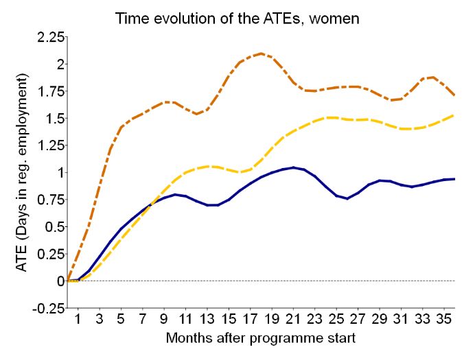
as in RIM and JT for both, men and women, the allocated participants to the programmes are

not the best choices, though differences are small. We investigate this more formally in the

course of the study.

 Panel B focuses on the long-term effects in the third year after the start of the programme.

We find every programme to be still beneficial for participants in the third year compared to

non-participation. Further, RIM, especially for men, unfolds its effect somewhat later and might

be even more beneficial if looking at a longer time-horizon.

 Figure 1: Evolution of ATE over time

Notes: Outcome is the cumulative days in regular employment for each month after start of participation in the
 respective programme. After month 4, all estimates are significantly different from zero at conventional
 levels. Exemplary, standard errors for month 10 (women: 0.19, 0.23, 0.31; men: 0.19, 0.23, 0.28), month
 20 (women: 0.24, 0.28, 0.37; men: 0.23, 0.27, 0.33), and month 30 (women: 0.25, 0.30, 0.39; men: 0.24,
 0.28, 0.33) for JT vs. NP, RIM vs. NP, and PS vs. NP, respectively.

 To complete the picture, Figure 1 presents how the effects of participation in the specific

programmes versus non-participation evolve over time. First to mention is that we do not

observe severe lock-in effects for any of the programmes. This is to be expected as the data

mainly covers long-term unemployed individuals, as described in Section 3, for whom it is hard

to find a job in general and who often show higher programme participation effects (see e.g.,

Blázquez, Herrarte, and Sáez (2019) for Spain). Second, the programmes’ durations are rather

short, i.e., programme participation holds off welfare recipients from job-search only for a short

time. Lastly, for women, PS is always the most beneficial, with a quick realisation period in the

first year and a rather constant benefit of about 1.6 - 2.0 more days in employment per month
 18

for participants after the first year. As PS is designed to push participants into the labour market,

this finding is not surprising. RIM steadily increases employment until 36 months after

participation. Such training programmes often unfold their effectiveness in particular in the

medium to long run (see Lorentzen and Dahl (2005) for Norway or the meta-analyses of Card,

Kluve, and Weber (2010, 2018)).

 The effect of JT increases to about 0.8 additional days in employment after nine months

and remains on this low level. Further, participation effects of this programme type often stay

rather constant in the medium to long run. For men, the picture is different. While in the first

months PS is the most beneficial programme, the effects of JT and RIM catch up and remain

close to each other. Especially the effect of PS is lower for men throughout, compared to women

(see similar findings in e.g., Bergemann and van den Berg (2008) and Dengler (2019)), leading

to a benefit of about 1.1 - 1.4 more days in employment per month for participating in any

programme for men in the long run.

 In the following, we investigate how the effects from Table 3 differ for the different

subpopulations of participants in the three programmes. The caseworkers are effective in

allocating individuals to programmes if the group of selected individuals to a specific treatment

benefit more from the treatment compared to the non-selected individuals. In other words, if

the ATET is larger than the ATE (or the average treatment effects of those groups selected to

none or a different training programme) the treated population is well selected. As already

described above for PS compared to non-participation, the caseworkers’ selection mechanism

tends to be effective, i.e., the ATET is larger than the ATE. For RIM and JT compared to non-

participation the selection mechanisms tend to be rather ineffective. Table 4 presents a formal

 19

WALD test for equality of the effects in all four subpopulations, i.e., the three participant groups

and non-participants. 10

 Table 4: Wald test of equality of effects in all four treatment specific subpopulations
 Cumulative months in JT vs. NP RIM vs. PS vs. NP RIM vs. PS vs. JT PS vs.
 employment NP JT RIM
 … in months 25 - 36 after start of treatment
 Women 29 9 24 37 6 2
 Men 80 99 61 98 98 90
 … in 36 months after start of treatment
 Women

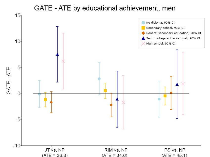
following, we focus on cumulative days in regular employment in three years, since the total

effect is likely to be most policy-relevant.

5.2.1 Group effects

 The analysis on the GATE level is of special policy interest and a good way to

systematically investigate treatment effects on an intermediate level. Using all available

potential variables for a heterogeneity analysis and reporting significant results only would be

datamining and surely the wrong way. We therefore pre-specified a short-list of variables of

special interest for policy makers, society, and academia in Table 5. 11

 Table 5: Short List - Wald tests for heterogeneity (p-values)
 Variable Women Men
 JT vs. NP RIM vs. NP PS vs. NP JT vs. NP RIM vs. NP PS vs. NP
 Personal characteristics
 Age§ 93 46 13 98 86 93
 Family status 3 73 1 16 58 59
 Educational 14 24 6 2 61 95
 achievement
 Days in reg. empl. 99 83 70 94 85 65
 in the prev. 5 years§
 Regional characteristics
 Region (East vs. 1 42

for differential effects. Significant differential effects in Table 5 can be found mainly for

women, specifically for JT and PS vs. NP. Variables indicated with “§” are discussed in the

following, while results for the other variables are shown in the Appendix.

 Due to historical reasons in many fields of the economy, there is still some discrepancy

between the former GDR region and the western part of Germany. It is therefore interesting to

analyse if training and job-search programmes are equally, more, or less effective in either of

those regions. We complement this by regional economic conditions, since the economic

conditions in East and West Germany are still very different, e.g., higher rates of unemployment

and less vacancies in the East. Further, especially important for the labour market authorities

are the labour market history of the individual as well as the age, since those are well observable

characteristics and might indicate the general potential of the unemployed. The third party

involved are the job centres, their structure and behaviour. Here, we are interested in the

influence of the sanction intensity, so how many sanctions are imposed in the specific job centre

as indication of the toughness of the caseworkers. All figures presented show differences of

GATEs to the respective ATE for women and men separately to investigate how those effects

differ compared to the average and with regard to gender. 12

 Figure 2 shows the results for the treatment effects of the programmes against non-

participation by regions. We find the effects for the group of individuals located in the western

part of Germany to be higher than for those located in the eastern part in every comparison.

Therefore, programmes in general seem to work better in West compared to East Germany.

Bernhard and Wolff (2008) found the same pattern for the contracting out to private placement

providers (programme replaced by PS). However, in our paper we found significantly

12
 To obtain the “pure” GATE, the ATE provided in each figure has to be added to the point estimate of the respective group.
 Since the vast majority of the GATEs are significantly different from zero, we opted for presenting the GATE-ATE to focus
 explicitly on within group differential effects.
 22

differential effects only for women in JT and PS compared to non-participation, while for men

the GATEs are all close to the population average effects.

 Figure 2: Difference of GATEs to ATE in West / East Germany

Notes: 90% confidence intervals (CI). ATE estimates in parentheses at the bottom of the graphs. Outcome is the
 cumulative days in employment in 36 months after start of treatment.

 To investigate if this is driven directly by the local economic conditions, which are worse

in East Germany compared to West Germany, we investigate the GATEs associated to the

district unemployment rate. Indeed, we find in general higher treatment effects for those female

participants in regions with a lower rate of unemployment, as shown in Figure 3. 13 As PS needs

vacancies to unfold its effectiveness and lower unemployment rates might be correlated with

higher amounts of available jobs, this finding is clear-cut. For men, the results of Figure 3 are

in line with the findings in Figure 2, as the GATEs fluctuate around the ATE. The same pattern

can be observed for GATEs associated to the unemployment rate of welfare recipients. Results

for this alternative measure of the labour market conditions can be found in Appendix C.3,

Figure 9.

13
 For the other treatment comparisons this tendency is equivalent, and the results can be found in Figure 8 in Appendix C.3.
 23

Figure 3: Difference of GATEs to ATE by district unemployment rate, PS vs. NP

Notes: 90% confidence intervals. ATE estimates in parentheses on the left-hand side of the graphs. Outcome is
 cumulative days in regular employment in 36 months after start of treatment. The green line represents
 the (kernel-)smoothed GATE estimates and is for illustration purposes only.

 For previous labour market success, in form of days in regular employment in the

previous five years, results can be found in Figure 11 in Appendix C.3. We do not find any

clear pattern. In addition, confidence intervals become increasingly large due to fewer

observations with many days in regular employment in the last five years. Thus, we refrain

from further interpretation.

 Figure 4: Difference of GATEs to ATE by age, RIM vs. JT

Notes: 90% confidence intervals. ATE estimates in parentheses on the left-hand side of the graphs. Outcome is
 cumulative days in regular employment in 36 months after start of treatment. The green line represents
 the (kernel-)smoothed GATE estimates and is for illustration purposes only.

 Another interesting question is if younger and older people should be sent to the same or

different ALMP. Figure 4 shows differential effects with individuals grouped by age for sending

them to RIM compared to JT. While for men it does not seem to matter, with all GATEs around

 24

the ATE, for women this does matter. Younger women should rather be allocated to the job-

training or non-participating (compare Figure 12 in Appendix C.3), older women benefit more

from the reducing impediments programme. For older men, instead, the placement services

programme seems to be more beneficial compared to non-participation, job-training or

reducing impediments, while the latter two are more beneficial for younger men; results for this

and the other comparisons can be found in Appendix C.3, Figure 12. That JT is more beneficial

for younger participants is in line with Caliendo and Schmidl (2016) who found positive effects

for young people participating in (solely) classroom-based training programmes (to which JT

is the most similar of our observed programmes).

 For job centres, imposing sanctions is a controversial tool to encourage means-tested

benefits recipients to actively search for jobs, take part in training programmes, etc. From an

academic point of view, it is interesting to investigate if those unemployed, who are supported

by job centres imposing more sanctions do benefit more or less from participation. Figure 5

provides results for being allocated to JT compared to not being allocated to one of the training

programmes associated to the job centres sanction intensity.

 Figure 5: Difference of GATEs to ATE by job centre sanction intensity, JT vs. NP

Notes: Job centres’ sanction intensity due to violations of duty. 90% confidence intervals. ATE estimates in
 parentheses on the left-hand side of the graphs. One outlier group is omitted for the sake of visibility. The
 full graph can be found in Appendix C.3, Figure 10. Outcome is cumulative days in regular employment
 in 36 months after start of treatment. The green line represents the (kernel-)smoothed GATE estimates
 and is for illustration purposes only.

 25

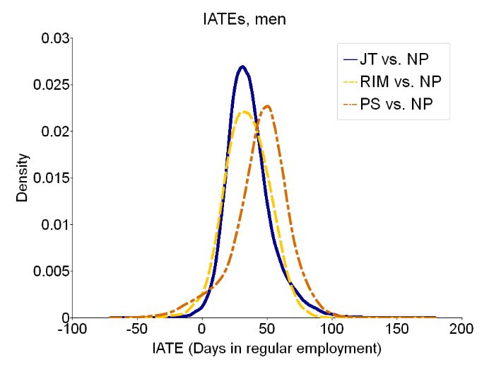
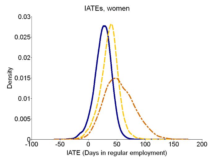
We find that for the effects for women associated to job centres with a higher sanctions’

intensity is indeed above the average effect, while those associated to a job centre imposing less

sanctions benefit below average. Again, for unemployed men there are no differential effects.

The same pattern is found for the comparison of the other treatments to non-participation and

results can be found in Figure 10 in Appendix C.3.

 To finally support the impressions already gained, that particularly for women, and less

for men, there is substantial effect heterogeneity we extend the set of heterogeneity variables to

a larger set in Appendix B. With this extended set we test every treatment comparison with a

WALD test for effect heterogeneity. We find several significant within-group differences of

effects for women (Table 12, Appendix B.1) and very few for men (Table 13, Appendix B.2).

This is all the more remarkable when one considers that we have fewer observations, and

therefore higher standard errors, for women than for men.

5.2.2 Individualised average effects

 On the lowest level of aggregation, Figure 6 presents the distributions of estimated IATEs

for participating in one of the treatments against non-participation. The first observation is that

for all labour market programmes most individuals realise positive effects. Table 6 documents

this with shares of 94.5 - 99.2 % of individuals having a positive effect from participating in

either programme. This is manifested in the substantial shares of individuals with significant

positive effects. Another conclusion from Figure 6 is that PS leads to the largest gains in days

in regular employment on average, like discussed in the previous subsection, as well as for a

substantial share of individuals.

 26

Figure 6: Distribution of estimated IATEs

Notes: IATE density plots. Outcome is the cumulative days in regular employment in 36 months after start of
 treatment.

 Table 6: IATEs, descriptions
 Women Men
 Share Share >0 Std SE Share Share >0 Std SE
 >0 (**) (aver.) >0 (**) (aver.)
 JT vs. NP 94.5 % 44.4 % 15.14 16.18 99.2 % 59.1 % 17.39 18.69
 RIM vs. NP 97.7 % 55.2 % 16.58 19.48 97.6 % 49.1 % 17.54 21.44
 PS vs. NP 99.0 % 63.8 % 26.85 24.53 95.7 % 57.6 % 21.98 24.98
Notes: Share of positive IATEs. Share significantly larger than zero indicated with ** on the 5% level. Std stands
 for the standard deviation of the respective distribution, SE (aver.) is the standard error averaged over all
 IATEs.

 Comparing the distributions of men with those of women, it is especially noteworthy that

the distribution of PS for women is wider as for man, as apparent from the standard deviations

(Std) shown in Table 6. This might be attributed to two aspects. It may point to some degree of

estimation error, since the estimation of IATEs is a much harder problem compared to the

estimation of average or group average effects. While Table 6 documents this showing for both

men and women the highest average standard errors for PS vs. NP, this cannot explain the wider

distribution for women compared to men. The remaining explanation is therefore that it points

to considerable effect heterogeneity in this programme and therefore high potential for a more

beneficial allocation of training programmes.

 An approach to describe those populations of individuals benefiting most and least from

ALMP participation is presented in Table 7. For this we show the dependence of the effects on

characteristics by k-means++ clustering (compare Arthur and Vassilvitskii (2007)). By jointly

 27

using the IATEs of participation in one of the programmes relative to non-participation, five

clusters are formed. Especially, those clusters are built by jointly sorting IATEs in increasing

order to find clusters, which represent the group of individuals benefiting most or least. The

fifth cluster represents the most affected individuals, i.e., those with the highest treatment

effects. In the first cluster, the least benefiting observations are grouped.

 Table 7: Descriptive statistics of clusters based on k-means clustering, IATEs
 Women Men
 Cluster Least Most Least Most
 beneficial beneficial beneficial beneficial
 Share of observations (in %) 13 27 13 12
 JT vs. NP 3 37 27 68
 RIM vs. NP 33 46 14 39
 PS vs. NP 8 49 7 55
 Personal characteristics
 Foreigner 0.20 0.25 0.26 0.22
 Days in regular employment (previous 5 265 84 704 201
 years)
 Days since last employment 1798 2244 453 1758
 No vocational / academic degree 0.49 0.65 0.47 0.47
 Vocational degree 0.47 0.31 0.49 0.42
 Academic degree 0.03 0.02 0.03 0.09
 Education - no schooling diploma 0.15 0.23 0.12 0.11
 Education - secondary school 0.40 0.45 0.50 0.39
 Education - general certificate of 0.33 0.21 0.27 0.23
 secondary education
 Education - advanced technical college 0.03 0.03 0.04 0.08
 entrance qualification
 Education - high school 0.07 0.05 0.07 0.15
 Marital status - unmarried 0.27 0.22 0.39 0.50
 Marital status - married 0.31 0.39 0.37 0.28
 Job centre characteristics
 Client-staff ratio in job centres 164 159 161 163
 Sanction intensity in job centres due to 0.45 0.62 0.58 0.53
 violations of duties (in percent)
 Sanction intensity in job centres due to 0.63 0.79 0.75 0.72
 failure in reporting (in percent)
 Regional characteristics
 District unemployment rate 11.3 9.6 9.8 10.5
 District unemployment rate of welfare 8.2 6.7 6.8 7.6
 recipients
 Region (west=0, east=1) 0.36 0.16 0.26 0.26
Notes: k-means++ clustering is used (Arthur and Vassilvitskii (2007)) with five clusters. Reported are clusters 1
 (least beneficial) and 5 (most beneficial), while the clusters 2-4 are reported in the full results in Tables 11
 (men) and 12 (women), which can be found in Appendix C.2. Average effects for the most and least
 benefiting populations for participating in one of the programmes compared to non-participation can be
 found in the top of the table. Outcome is the cumulative days in regular employment in 36 months after
 start of treatment.

 28