An Advection-Reflection Solver for Detail-Preserving Fluid Simulation - Jonas Zehnder
←
→
Page content transcription
If your browser does not render page correctly, please read the page content below
An Advection-Reflection Solver for Detail-Preserving Fluid Simulation
JONAS ZEHNDER, Université de Montréal
RAHUL NARAIN, University of Minnesota and Indian Institute of Technology Delhi
BERNHARD THOMASZEWSKI, Université de Montréal
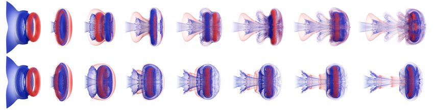
Fig. 1. Our new reflection solver applied to a vortex leap-frogging problem (top row). During 10s of simulation the two vortex rings move through each other
multiple times and stay well separated. By contrast, in a standard advection-projection method with MacCormack advection (bottom row), the two vortices
merge immediately and never separate afterwards.
Advection-projection methods for fluid animation are widely appreciated Graph. 37, 4, Article 85 (August 2018), 8 pages. https://doi.org/10.1145/
for their stability and efficiency. However, the projection step dissipates 3197517.3201324
energy from the system, leading to artificial viscosity and suppression of
small-scale details. We propose an alternative approach for detail-preserving 1 INTRODUCTION
fluid animation that is surprisingly simple and effective. We replace the
energy-dissipating projection operator applied at the end of a simulation Advection-projection methods are widely used for fluid animations
step by an energy-preserving reflection operator applied at mid-step. We show in computer graphics. Splitting mass transport and conservation
that doing so leads to two orders of magnitude reduction in energy loss, into different steps allows for stable and efficient integration, and
which in turn yields vastly improved detail-preservation. We evaluate our advances in higher-order advection schemes (e.g. [Selle et al. 2008])
reflection solver on a set of 2D and 3D numerical experiments and show have greatly reduced the well-known numerical diffusion caused
that it compares favorably to state-of-the-art methods. Finally, our method by the semi-Lagrangian advection step. However, the splitting of
integrates seamlessly with existing projection-advection solvers and requires the time integration scheme itself induces numerical dissipation, as
very little additional implementation.
kinetic energy is transferred to divergent modes during advection
CCS Concepts: • Computing methodologies → Physical simulation; and then lost after projection. This numerical dissipation manifests
Computer graphics; Animation; as rapid decay of large vortices and leads to suppression of small-
Additional Key Words and Phrases: fluid simulation, advection, reflection, scale swirling motion. Since visual complexity is a central goal in
energy conservation fluid animation, much effort has been spent on combating numerical
dissipation: apart from higher-order advection schemes mentioned
ACM Reference Format:
above, energy-preserving integration [Mullen et al. 2009], a pos-
Jonas Zehnder, Rahul Narain, and Bernhard Thomaszewski. 2018. An Advec-
tion-Reflection Solver for Detail-Preserving Fluid Simulation. ACM Trans.
teriori correction of the velocity field [Fedkiw et al. 2001; Zhang
et al. 2015], and injection of procedurally-generated detail [Kim et al.
Authors’ addresses: Jonas Zehnder, Université de Montréal, jonas.zehnder@umontreal. 2008b] are among the strategies that have been pursued so far.
ca; Rahul Narain, University of Minnesota, Indian Institute of Technology Delhi,
narain@cse.iitd.ac.in; Bernhard Thomaszewski, Université de Montréal, bernhard@iro.
In this work, we propose an alternative approach to detail-pre-
umontreal.ca. serving fluid animation that is surprisingly simple and effective: we
replace the energy-dissipating projection operator applied at the
Permission to make digital or hard copies of all or part of this work for personal or end of a simulation step by an energy-preserving reflection operator
classroom use is granted without fee provided that copies are not made or distributed
for profit or commercial advantage and that copies bear this notice and the full citation applied at mid-step; see Fig 2. We show that doing so leads to an
on the first page. Copyrights for components of this work owned by others than the order of magnitude reduction in divergent kinetic energy, which in
author(s) must be honored. Abstracting with credit is permitted. To copy otherwise, or
republish, to post on servers or to redistribute to lists, requires prior specific permission
turn leads to vastly improved preservation of vortices and small-
and/or a fee. Request permissions from permissions@acm.org. scale detail. This analysis also exposes our method to be first-order
© 2018 Copyright held by the owner/author(s). Publication rights licensed to Association structurally symmetric, which motivates an analogy to (and compar-
for Computing Machinery.
0730-0301/2018/8-ART85 $15.00 ison with) symmetric projection methods for structure-preserving
https://doi.org/10.1145/3197517.3201324 integration of constrained mechanical systems [Hairer et al. 2006].
ACM Transactions on Graphics, Vol. 37, No. 4, Article 85. Publication date: August 2018.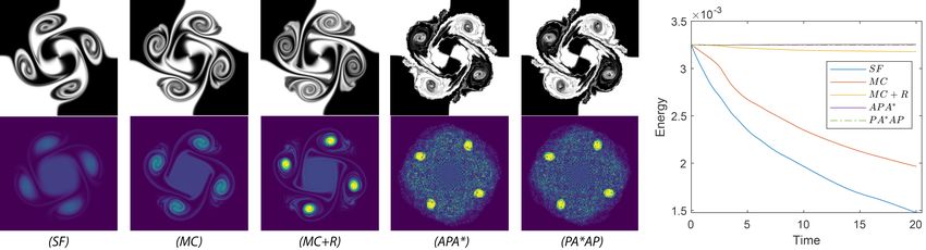
85:2 • J. Zehnder, R. Narain, and B. Thomaszewski

                     ũ1                                                                       As discussed in the introduction, there are two main reasons for
                                        ũ1/2                        ũ1/2                 the loss of energy in an advection-projection method: the discretiza-
                                                                                ũ1
                                                                                           tion error in the semi-Lagrangian advection step, which manifests
                                                   u1                                      as artificial diffusion, and the splitting error caused by decoupling of
 u0                  u1        u0                           u0       u1/2       u1         the advection and projection steps. To reduce the diffusion in semi-
                                                   ũ1                                     Lagrangian advection, Fedkiw et al. [2001] and Kim et al. [2008a]
                                        û1/2                                              have proposed higher-order interpolation schemes to improve spa-
                                                                                           tial accuracy. Kim et al. [2005, 2007] introduced the BFECC method
Fig. 2. A geometric interpretation of our method. Left: In a standard advec-               which performed multiple backward and forward advection steps to
tion-projection solver, projection to the divergence-free subspace causes                  correct both spatial and temporal error. This approach was simpli-
kinetic energy loss (red). Middle: Our reflection solver uses an energy-                   fied by Selle et al. [2008], who proposed a semi-Lagrangian variation
preserving reflection (yellow) halfway through the advection step, dramati-                of the MacCormack method and demonstrated second-order accu-
cally reducing the energy loss caused by the final projection. Our method
                                                                                           racy in space and time. Molemaker et al. [2008] proposed the use of
has effectively identical computational cost to an advection-projection solver
with half the time step (right), but loses less energy.
                                                                                           the QUICK advection scheme [Leonard 1979] for low-dissipation
                                                                                           advection, although it is limited by the CFL condition for stability.
                                                                                           In this context, hybrid particle-and-grid methods like FLIP [Zhu and
                                                                                           Bridson 2005] and APIC [Jiang et al. 2015] are very attractive as they
We show that even the simplest methods from this category are com-                         exhibit little numerical diffusion of this form, because they track
putationally much more expensive and less stable. By contrast, our                         the advected quantities on Lagrangian particles which are largely
method preserves the appreciable splitting property of advection-                          unaffected by the grid interpolation.
projection methods while offering energy and detail preservation                               In contrast to the improvements in low-diffusion advection
similar to fully-symmetric methods.                                                        schemes, much less attention has been paid to the error introduced
   Our method integrates seamlessly with existing advection-pro-                           by the splitting scheme itself. In graphics, this has been pointed
jection solvers and is agnostic to the choice of advection scheme                          out by Elcott et al. [2007] and Zhang et al. [2015], who noted that
and pressure discretization. Furthermore, it uses the basic advection                      semi-Lagrangian advection transfers energy into divergent modes
and projection steps as primitives, and therefore requires very little                     which are then annihilated by the projection step. This is true even
additional implementation. We evaluate our reflection solver on an                         for the FLIP and APIC methods, which employ the same advection-
extensive set of 2D and 3D examples and compare its behavior to a                          projection splitting. Elcott et al. instead adopted the vorticity for-
number of alternative methods. The results of these comparisons                            mulation of the fluid equations, in which the primary variable is
indicate that, for equal computational costs, our method leads to                          the vorticity rather than the velocity field. Other vorticity-based
vastly improved energy and vorticity preservation.                                         methods in graphics include Angelidis and Neyret [2005]; Park and
                                                                                           Kim [2005]; Weißmann and Pinkall [2010]. Since the vorticity repre-
                                                                                           sentation automatically yields a divergence-free velocity field, such
2     RELATED WORK                                                                         methods do not require a projection step, and consequently do not
Our review of related works focuses primarily on Eulerian fluid                            suffer the associated energy loss. Particularly notable is the method
simulation methods, as our approach does not apply to Lagrangian                           of Mullen et al. [2009], which is time-reversible and offers exact en-
particle-based methods like SPH [Ihmsen et al. 2014]. Also, we will                        ergy preservation through the use of a symplectic integrator, albeit
only discuss schemes for solving the core Navier-Stokes equations,                         at the cost of requiring the solution to a nonlinear system at each
omitting the diversity of techniques in graphics for artificially inject-                  time step. Nevertheless, advection-projection methods continue to
ing detail such as vorticity confinement [Fedkiw et al. 2001], vortex                      enjoy widespread use in industry and academic research, possibly
particles [Selle et al. 2005], and turbulence synthesis [Thuerey et al.                    due to their relative simplicity, efficiency, and flexibility in compari-
2013].                                                                                     son to vorticity methods [Zhang et al. 2015]. Therefore, we believe
   Most Eulerian methods in graphics follow a Chorin-style advec-                          that advances in energy preservation for advection-projection meth-
tion-projection scheme [Chorin 1968] introduced to graphics by                             ods are still highly desirable.
Stam [1999]. The effectiveness of the advection-projection approach                            Remaining within the advection-projection framework, Zhang
stems from three main ingredients: (i) operator splitting decouples                        et al. [2015] counteracted the artificial dissipation caused by the pro-
the pressure term from the remaining inertial and internal forces, (ii)                    jection step by explicitly tracking the lost vorticity and re-injecting
semi-Lagrangian advection [Robert 1981] permits large time steps                           it into the fluid. Thus, their work seeks to preserve vorticity but not
unimpeded by the CFL condition, and (iii) staggered grids [Foster                          necessarily the energy of the fluid. In contrast, we propose a simple
and Metaxas 1996; Harlow and Welch 1965] allow for accurate                                modification to the splitting scheme which reduces the projection
computation of the pressure projection. While this approach is                             error without requiring explicit tracking and correction. We also
unconditionally stable, it exhibits noticeable energy loss over time                       provide a simple proof that our scheme preserves kinetic energy to
even for inviscid flows. Small-scale vortices and turbulent flows tend                     a higher degree than traditional advection-projection methods.
to decay especially rapidly, leading to a loss of visually interesting
detail. Much work in computer graphics has focused on minimizing
this numerical dissipation.

ACM Transactions on Graphics, Vol. 37, No. 4, Article 85. Publication date: August 2018.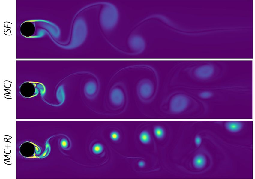
An Advection-Reflection Solver for Detail-Preserving Fluid Simulation •                        85:3

3      THEORY                                                                              as ∇ · ũ = δ ∆t k + o(∆t k ) for some scalar field δ . Thus we have
                                                                                           1 ∥v∥ 2 = 1 ∥Hδ ∥ 2 ∆t 2k + o(∆t 2k ) = Θ(∆t 2k ).
To set the stage for our theoretical developments, we start with a                         2         2
minimal review of advection projection methods before we intro-                              Using this result, we show that an advection-projection solver
duce our reflection solver. For context and comparison, we subse-                          can at best only preserve energy to first order in time.
quently introduce two fully-symmetric projection methods.
   For notational convenience, we will refer to the velocity field                           Theorem 2. The kinetic energy loss due to the projection step of
at the beginning and end of the time step as u0 and u1 respec-                             the advection-projection method is Θ(∆t 2 ).
tively, instead of un and un+1 . We will also adopt the convention                            Proof. Expanding the advection operator into its Taylor series,
that divergence-free velocity fields are undecorated, e.g. u1/2 , while
velocity fields with nonzero divergence are denoted ũ (before pro-                                             ũ1 = u0 − (u0 · ∇)u0 ∆t + O(∆t 2 ).                        (3)
jection) or û (after reflection).                                                         we find that the divergence of the advected velocity field is
                                                                                                         ∇ · ũ1 = ∇ · u0 − ∇ · ((u0 · ∇)u0 )∆t + O(∆t 2 )                  (4)
3.1     Advection-Projection Solvers
The starting point for our developments are the inviscid, incom-                                                 = −∇ · ((u · ∇)u ) ∆t + O(∆t ).
                                                                                                                                 0      0               2
                                                                                                                                                                            (5)
                                                                                                                   |      {z     }
pressible Navier-Stokes equations                                                                                             δ (u0 )
                         ∂u               1                                                For a divergence-free velocity field u, it can be shown that the rate
                            + (u · ∇)u = − ∇p + f                                (1)
                         ∂t               ρ                                                of divergence δ (u) is proportional to the second invariant of the
                                 ∇·u=0,                                          (2)                         Í ∂ui ∂u j
                                                                                           velocity gradient, i j ∂x ∂x , and is not in general zero. Therefore,
                                                                                                                          j       i
where u is the continuous velocity field of the fluid, p is the pressure,                  we have ∇ · ũ1 = Θ(∆t), resulting in an energy loss of order Θ(∆t 2 ).
ρ the density and f denote external forces such as buoyancy and
gravity. Advection-projection methods discretize the velocities on a
Eulerian grid and split the equations into three (or more) different                       3.2    Reflection Solver
steps:                                                                                     We would like to avoid the second-order energy loss during pro-
                                                                                           jection while still achieving zero divergence at the end of the time
                     Advection          ũ1 = A(u0 ; u0 , ∆t)
                                                                                           step. The intuition for our approach is that, instead of correcting
                        Forcing         ũ1 += ∆t f                                        the velocity at the end of the time step, we can over-compensate
                     Projection         u1 = P ũ1 .                                       in the middle: we advect to the middle of the time interval and
                                                                                           apply twice the correction needed to obtain a divergence-free field
In the above expressions, A(u; u0 , ∆t) is an advection operator that                      such as to anticipate the divergence incurred during the second half.
implements a semi-Lagrangian discretization of the advection equa-                         Geometrically, this operation can be interpreted as symmetrically
tion, ∂u
      ∂t + (u · ∇)u = 0. Furthermore, P is a projection operator
              0                                                                            changing from one side of the divergence-free manifold to the other,
that maps a given velocity field to its closest divergence-free field                      hence the term reflection; see Fig. 2. Concretely, the reflection solver
(under the kinetic energy metric). This operator uses the Helmholtz-                       proceeds as follows:
Hodge decomposition, which splits any vector field u = v + w into
                                                                                                                     ũ1/2 = A(u0 ; u0 , 12 ∆t)
a curl-free part v and a divergence-free part w. P simply discards
the curl-free part, Pu = w, by solving a Poisson problem.                                                            u1/2 = P ũ1/2
   For conciseness, we will neglect the forcing step in the following                                                û1/2 = 2u1/2 − ũ1/2
and focus on the central advection and projection steps. In practice,
we apply external forces immediately after each advection.                                                              ũ1 = A(û1/2 ; u1/2 , 21 ∆t)

  Lemma 1. If a vector field ũ has divergence Θ(∆t k ), the kinetic                                                    u1 = P ũ1 .
energy loss due to projection, 12 ∥ ũ∥ 2 − 21 ∥P ũ∥ 2 , is Θ(∆t 2k ).                    As it is preferable to perform semi-Lagrangian advection using
                                                                                           a divergence-free velocity field (otherwise the advection equation
    Proof. The pressure projection can be interpreted as decom-                            does not correspond to a conservation law for the advected quantity),
posing the post-advection velocity ũ into two orthogonal com-                             we use the projected mid-step velocity u1/2 in the second semi-
ponents, ũ = P ũ + v, where v is the curl-free part. Due to the                          Lagrangian advection step. Note that the reflection velocity û1/2
orthogonality of the Helmholtz-Hodge decomposition, we have                                can also be written directly as û1/2 = R ũ1/2 , where R = 2P − I is
∥ ũ∥ 2 = ∥P ũ∥ 2 + ∥v∥ 2 . Therefore, the energy loss 12 ∥ ũ∥ 2 − 12 ∥P ũ∥ 2           the reflection operator. The final projection u1 = P ũ1 guarantees
is precisely the kinetic energy of the curl-free part, 12 ∥v∥ 2 . Fur-                     divergence-free velocity at the end of the time step. However, if the
thermore, the curl-free part v is determined by the divergence of                          rate of divergence does not vary much across the time step, then
ũ and depends linearly on it; that is, we can write v = H (∇ · ũ)                        ũ1 will already be close to divergence-free. Indeed, this intuition is
for some linear operator H .1 If ∇ · ũ = Θ(∆t k ), it can be expressed                    confirmed by the following statement.
1 Inparticular, H = ∇∆−1 , where ∆−1 denotes the inverse of the Laplace operator with        Theorem 3. The kinetic energy loss due to the projection step of
the appropriate problem-defined boundary conditions.                                       the reflection solver is O(∆t 4 ).

                                                                                        ACM Transactions on Graphics, Vol. 37, No. 4, Article 85. Publication date: August 2018.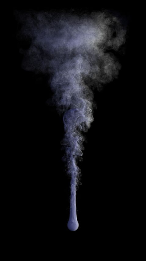
85:4 • J. Zehnder, R. Narain, and B. Thomaszewski

  Proof. Using the Taylor series expansion of the advection oper-                          3.3   Symmetric Projection Methods
ator, we approximate the mid-step velocities as                                            The results of the previous section suggest that our reflection solver
                  ũ1/2 = u0 − (u0 · ∇)u0 ∆t/2 + O(∆t 2 ) ,                      (6)       is first-order structurally symmetric: even though the advection oper-
                                                                                           ator itself is not, the structure of the advection-reflection-advection
                   1/2
                  û     = u − R(u · ∇)u ∆t/2 + O(∆t ) ,
                             0       0        0                2
                                                                                 (7)       sequence is symmetric. This observation prompted us to draw the
                                                                                           analogy to symmetric manifold projection methods, a class of in-
where we have used the fact that Ru0 = u0 since u0 is already
                                                                                           tegrators for conservative mechanical systems known for their ex-
divergence-free. An analogous first-order approximation of the end-
                                                                                           cellent long-term energy conservation [Hairer et al. 2006]. Indeed,
of-step velocity before projection, ũ1 , yields
                                                                                           by composing the advection-projection step with its adjoint—and
     ũ1 = û1/2 − (u1/2 · ∇)û1/2 ∆t/2 + O(∆t 2 )                               (8)       vice-versa—we obtain two immediate candidates for symmetric
                                                                                           advection-projection schemes.
         = u0 − R(u0 · ∇)u0 ∆t/2

                                                                                 (9)
                                                                                              We start by defining some key terms, following Hairer et al. [2006].
          − (u0 + O(∆t)) · ∇ u0 + O(∆t) ∆t/2 + O(∆t 2 )                                    The adjoint of a time-stepping scheme Φ( · , h) is the inverse of its

                                                                                (10)
         = u − R(u · ∇)u ∆t/2 − (u · ∇)u ∆t/2 + O(∆t )
              0          0       0           0        0                2
                                                                                (11)       time reversal, Φ∗ ( · , h) = Φ−1 ( · , −h). A time-stepping scheme is
                                                                                           symmetric, or time-reversible, if it is equal to its adjoint. Compos-
         = u0 − 2P (u0 · ∇)u0 ∆t/2 + O(∆t 2 ) .

                                                                                (12)       ing any consistent first-order scheme Φ with its adjoint yields a
                                                                                           symmetric second-order scheme, Ψ( · , h) = Φ∗ ( · , h/2) ◦ Φ( · , h/2).
From this, it is evident that ũ1 is divergence-free to first order,
                                                                                              Strictly speaking, the adjoint of the pressure step does not exist
i.e. ∇ · ũ1 = O(∆t 2 ). Therefore, the resulting energy loss is of order
                                                                                           because P as a linear operator is not invertible. In this section, we
O(∆t 4 ).
                                                                                           interpret P as an arbitrary perturbation normal to the divergence-
  The good energy-preserving properties of our reflection solver                           free manifold, defining P(u; p) = u − ∇p for any pressure field p.
are further assured by the fact that                                                       This operation is self-adjoint: P ∗ (u; p) = P −1 (u; −p) = P(u; p).

   Theorem 4. The reflection operator preserves kinetic energy.                              APA∗ . The first scheme is obtained by composing the advection-
                                                                                           projection step, AP, with its adjoint PA∗ . Geometrically, we first
   Proof. The pressure projection w = Pu can be interpreted as                             advect to the middle of the time step to obtain ũ1/2 and project onto
finding w as the closest point to u in the space of divergence-free                        the divergence-zero manifold. To implement PA∗ , we solve for a
vector fields, under the metric defined by kinetic energy [Batty et al.                    pressure field p used to compute velocity perturbations ∆up = −∇p
2007]. Consequently, P is an orthogonal projection with respect to                         normal to the manifold, as well as divergence-free end-of-time-step
kinetic energy,∭and v and w are orthogonal to each other in the sense                      velocities u1 such that, when advecting u1 backward in time, we
that ⟨v, w⟩ =     ρv·w dV = 0. Using the definition of the reflection                      end up at the perturbed mid-step velocities û1/2 = ũ1/2 − ∇p. This
operator, we have for the reflected velocity field Ru = 2w−u = w−v.                        sequence of coupled operations translates into a system of nonlinear
Comparing the kinetic energies, we find that                                               equations,
               1           1                   1
                 ⟨Ru, Ru⟩ = (⟨w, w⟩ + ⟨v, v⟩) = ⟨u, u⟩.                                                A(u1 ; u1 , − 12 ∆t) − (A(u0 ; u0 , 12 ∆t) − ∇p) = 0

                                                                                (13)
                                                                                                                                                              . (14)
               2           2                   2                                                                            ∇ · u1 = 0

                                                                                           in which the projection and perturbation steps combine into a single
   These results also point to the stability of our method, since                          operation, which is why we mnemonically refer to this scheme as
the reflection operator preserves energy, while the final projec-                          APA∗ . We note that this system is similar to the one derived by
tion can only reduce it. In conjuction with the stability of semi-                         Mullen et al. [2009]. We solve (14) with Newton’s method and, as do
Lagrangian advection operations, one would like to argue that the                          Mullen et al., approximate the Jacobian of the advection operator
reflection method is unconditionally stable. This argument does not                        with the identity matrix. When applying block Gaussian elimination
go through smoothly, however, as advection is stable in a slightly                         to the resulting saddle-point systems, we recover the same Poisson
different sense: it is monotonic in the field values, not necessarily                      problem encountered in standard advection-projection methods,
in energy. However, the same caveat applies to all other advection-
projection solvers used in graphics. As such we expect to see un-                                                  ∇2 (∆p) = ∇ · rAP A∗ ,                      (15)
conditional stability in practice, independent of the time step size.                      albeit with a different right hand side rAP A∗ that we omit here for
   It is worth noting here that the reflection solver does not neces-                      brevity. This pressure solve must be performed once per Newton
sarily improve the accuracy of the solution over projection solvers,                       iteration, providing us with updated perturbations ∆p and corre-
since it still incurs error due to self-advection using a “frozen” veloc-                  sponding velocity updates.
ity field. For time-varying flows the method remains only first-order
accurate in time, as we show in Section 4.3. Instead, the benefit                             PA∗AP. The second scheme is obtained by composing the adjoint
of the reflection approach is a higher degree of energy conserva-                          of the advection-projection step with itself, leading to the mnemonic
tion. This is analogous to how BDF2 and implicit midpoint are both                         sequence PA∗AP. As a geometric interpretation, we solve for pertur-
second-order accurate integration schemes, but implicit midpoint                           bations p and mid-step velocities u1/2 such that 1) advecting from
has significantly better conservation properties.                                          the middle to the end and applying the correction −∇p leads to

ACM Transactions on Graphics, Vol. 37, No. 4, Article 85. Publication date: August 2018.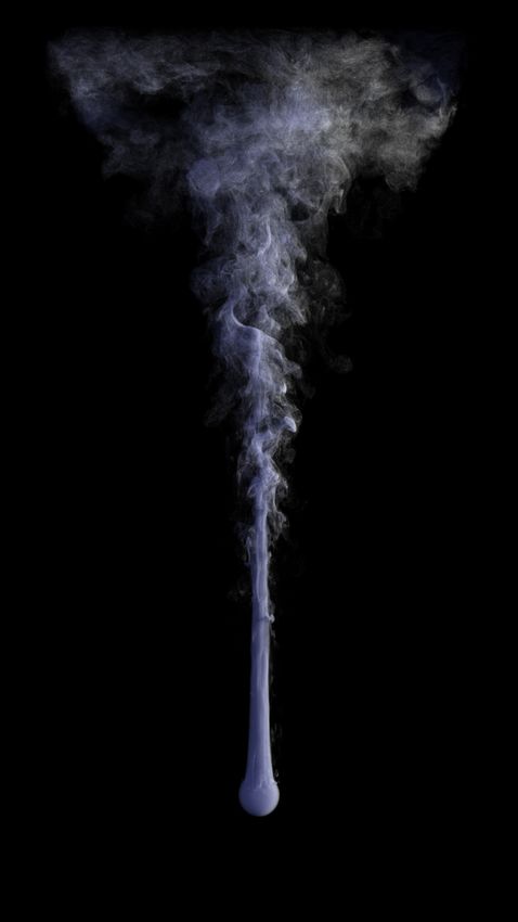
An Advection-Reflection Solver for Detail-Preserving Fluid Simulation •                        85:5

Fig. 3. 2D vortex sheet example: comparison of the density distribution (top) and the vorticity magnitude (bottom) for a fixed point in time (10s) as obtained
for the various solvers. Far right: kinetic energy as a function of time.

divergence-free velocities, and 2) advecting from the middle back-                Pfaff 2016], which we modified slightly to implement our reflection
wards leads to the perturbed initial velocities u0 − ∇p. Combining                solver.
these operations together leads to a system of nonlinear equations,                  We compare the following solvers: stable fluids with first-order
                                                                                  semi-Lagrangian advection (SF) as described by Stam [1999], stable
                A(u1/2
                      ; u , − 2 ∆t) − u − ∇p     =0
             (            1/2   1            0
                                                                                  fluids with MacCormack advection (MC) [Selle et al. 2008], our reflec-
                                                               (16)
                  ∇ · A(u1/2 ; u1/2 , 12 ∆t) − ∇p = 0                             tion solver (R), as well as the symmetric projection methods (APA∗ )
                                                                                  and (PA∗AP). Statistics on all experiments and solvers—including
that we solve for the mid-step velocities u1/2 and the unknown per-               step size, grid size, and computation time—are listed in Table 1.
turbation field p using Newton’s method. This scheme is analogous                 Since our reflection solver requires two advection operations and
to the symmetric projection method describe by Hairer et al. [2006]               two pressure solves per time step, we use twice the step size when
and, upon approximation of the Jacobian with the identity matrix                  comparing to SF and MC, giving us essentially identical computation
and block Gaussian elimination, leads again to a standard pressure                time.
solve (the details of which we leave out for conciseness).
                                                                                  4.1    2D Results
   Discussion. We provide qualitative and quantitative evaluations
for these symmetric projection methods in Section 4 and compare                   Since two-dimensional flows are generally easier to interpret and
them to our reflection solver. But even before further analysis, we               compare, we begin our analysis in the 2D setting.
can already expect these methods to have much higher computa-
                                                                                     2D Vortex Sheet. We initialize a disc-shaped region in the center
tional cost than our reflection solver: solving the systems to suffi-
                                                                                  of the scene with a rigid rotation as the initial velocity field. After
cient accuracy requires several Newton iterations, each with one
(resp. two) advection steps and a pressure solve. Furthermore, while
the use of an approximate Jacobian is justified by the difficulty of
computing the full Hessian, it warrants the use of line search for                Table 1. (1) 2D Vortex Sheet, (2) Taylor Vortices, (3) Vortex Shedding, (4)
convergence control. However, since the systems of equations do                   Spiral Maze, (5) Vortex Leap-Frogging, (6) Ink Drop, (7) Smoke Plume, (8)
not derive from a minimization problem with associated objective                  Smoke Plume with Sphere
function, we can only monitor the norm of the residual—a poor                     The time step was doubled for the reflection solver when producing the
                                                                                  results to keep cost similar to the projection method. The time step was
measure of progress that can even prevent convergence.
                                                                                  reduced for P A∗ AP and AP A∗ to satisfy the CFL condition.

4   RESULTS
                                                                                                                                                     Iter. time (s)
We investigated the qualitative and quantitative behavior of our                            Resolution            Domain size               ∆t
reflection solver on a set of 2D and 3D experiments commonly                                                                                          MC MC+R
used in the literature. We compare our results to those obtained for                1      256 × 256                  1×1               0.025      0.0281       0.055
conventional advection-projection solvers and report our findings                   2      256 × 256                  1×1               0.025      0.0285       0.055
below.                                                                              3      512 × 128                1 × 0.25           0.0025      0.0322      0.0638
                                                                                    4      256 × 256              0.75 × 0.75           0.025      0.0558      0.1107
  Solvers & Setup. For the 2D experiments, we use our own solver                    5   256 × 128 × 128         256 × 128 × 128          0.25         5.59      10.43
based on a MAC grid discretization. To implement internal obstacles                 6    128 × 64 × 64           128 × 64 × 64              1         0.27        0.57
in the flow, we use the method of Batty et al. [2007] and apply                     7   128 × 256 × 128         128 × 256 × 128             1         5.73      10.66
corresponding modifications to the matrix of the pressure solves.                   8   128 × 256 × 128         128 × 256 × 128             1         7.97      13.48
The 3D examples are based on the Mantaflow library [Thuerey and

                                                                               ACM Transactions on Graphics, Vol. 37, No. 4, Article 85. Publication date: August 2018.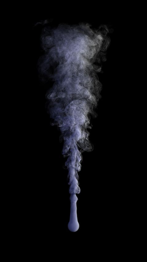
85:6 • J. Zehnder, R. Narain, and B. Thomaszewski
Fig. 4. 2D Taylor vortices. Left: initial vorticity magnitude and results for
the three solvers after 10s. Right: kinetic energy as a function of time.
initialization, no additional energy is injected into the system, allow- Fig. 5. 2D vortex shedding: comparison of the vorticity magnitude distribu-
ing us to investigate the (long-term) energy conservation properties tions for SF, MC, and MC+R for a fixed point in time (6s).
of the different solvers.
Fig. 3 shows an overview of density and vorticity magnitude fields
obtained for the various solvers applied to this problem. While the
differences in dynamic behavior are best observed in the accompa-
nying video, it can be seen that our reflection solver MC+R shows
slightly better detail preservation in the density field than MC and
much less vorticity diffusion. Moreover, the temporal evolution of
kinetic energy shown in Fig. 3 (right) speaks a very clear language:
SF rapidly dissipates energy, which drops to two thirds of its initial
value after roughly 6s. MC performs better, but still loses one third of Fig. 6. A vortex in a spiral maze (left) correctly advects itself to the center
its energy after 13s. By contrast, our reflection solver preserves en- (right).
ergy much better, losing less than 3% over the entire animation (20s).
For reference, the symmetric projection methods both preserve en-
ergy perfectly, but they require roughly 10 times more computation dynamic and visually rich vortex shedding. As can be seen from Fig.
time. What is worse, however, is that both methods lead to visually 5, MC initially produces similar behavior in the sense that roughly
disturbing artifacts in the density field and very noisy vorticity (see the same number of vortices is shed during the first 6 seconds.
Fig. 3). We have investigated this behavior intensively but could However, whereas our reflection solver approximately preserves
not find a problem with our implementation. We conjecture that the vorticity of the shed vortices, there is a clear decay in vorticity
the reason for these artifacts lies in the semi-Lagrangian advection (from left to right) for MC. The video also shows that the behavior
operator: the interpolations performed when tracing back through for SF is qualitatively very different and the numerical viscosity is
the velocity field act as a low-pass filter, i.e., information is lost due clearly visible.
to interpolation. Although the continuity of the flow provides some Spiral Maze. An example introduced by Mullen et al. [2009] con-
amount of regularization, the effective inversion of this low-pass tains a pair of vortices in a 2D domain with many boundaries form-
filter during A∗ is numerically unstable, explaining both the arti- ing a spiral maze. In the absence of dissipation, one of the vortices
facts and the intermittent convergence problems that we observed. should advect itself to the center of the maze. As shown in Fig-
Although we intended these symmetric methods to be reference so- ure 6, our method produces the expected behavior. Interestingly,
lutions, we found them to be unusable in practice and will therefore unlike the results of Mullen et al., we also observe additional vortex
not discuss them further. shedding due to flow separation at the convex corners of the maze.
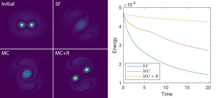
Taylor Vortices. Another frequently used 2D example is that of two
vortices of the same sign placed at a given initial distance. Depending 4.2 3D Results
on this initial distance, the analytical solution for this problem will To investigate the behavior of our reflection solver in 3D, we chose
lead to the vortices either merging or separating. Following Mullen a set of examples frequently used in the literature.
et al. [2009], we choose the initial distance slightly larger than the
Vortex Leap-Frogging. This classical example is initialized with
critical value and investigate the behavior of the solvers. For both
two concentric vortex rings of different radii but equal circulations.
SF and MC, the vortices merge shortly after the beginning of the
In the analytical solution for the completely inviscid, conservative
simulation, whereas they separate as predicted by the analytical
case, the two vortices will produce a leap-frogging motion that
solution using our reflection solver.
continues indefinitely. However, reproducing this behavior with
Vortex Shedding. This example investigates the behavior of the Eulerian methods has been a challenging problem due to the ten-
different solvers in combination with internal boundaries, leading to dency for numerical dissipation to diffuse the vortices into each
ACM Transactions on Graphics, Vol. 37, No. 4, Article 85. Publication date: August 2018.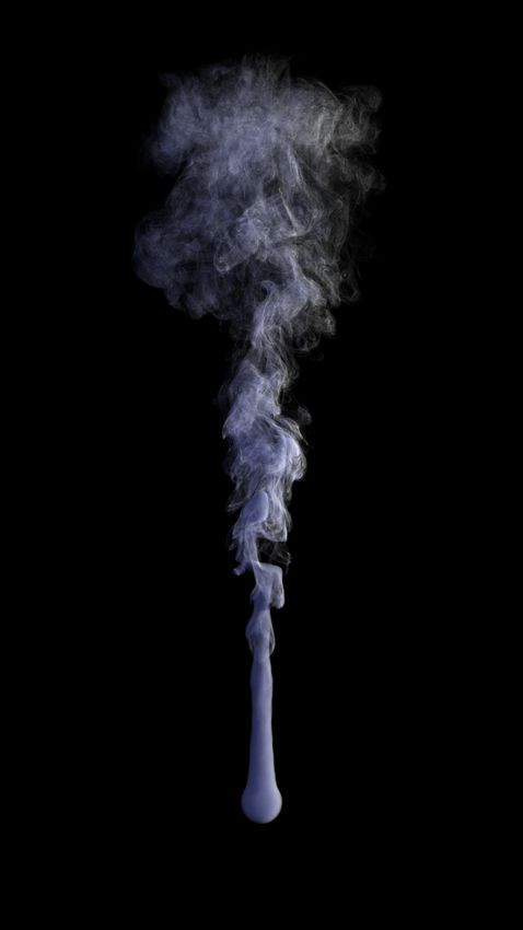
An Advection-Reflection Solver for Detail-Preserving Fluid Simulation •                                                     85:7

                                                                                                                          100

                                                                                                                         10-2

                                                                                                            Divergence
                                                                                                                         10-4

                                                                                                                         10-6

                                                                                                                         10-8

                                                                                                                         10-10
                                                                                                                                  10-4            10-3             10-2          10-1   100

           SF                      MC                      FLIP
                                                                               Fig. 8. Norm of the divergence before the projection step for different step
Fig. 7. 3D smoke plume with different advection schemes. In each pair, we      sizes and different solvers. Reverse Limiter refers to the clamping of the
compare the same simulation frame computed using a standard projection         interpolated field value in the MacCormack scheme.
solver (left) and our reflection solver (right).

                                                                               solver, however, the decrease is indeed quadratic, irrespective of
other. As can be seen in Fig. 1, when using the MC solver, the vortex          whether it is combined with first order or MacCormack advection.
rings merge into a single one during the first leap-through motion.            Another observation that we made in this context is that because
By contrast, our solver successfully produces several leap-frogging            in this test we only increased the resolution in time, not in space,
moves in which the rings remain clearly separated. We refer to                 clamping the interpolated field value in the MacCormack scheme
the accompanying video for a better illustration of this fascinating           slows the convergence of the norm of the divergence.
phenomenon.                                                                       To evaluate the accuracy of our method, we performed a conver-
                                                                               gence test using a 2D Taylor-Green vortex with initial conditions
   Ink Drop. A spherical density field is initialized with constant
horizontal velocity. Using our reflection solver, the velocity gradient                                   uTG = (sin(2πx) cos(2πy), − cos(2πx) sin(2πy)).
at the sphere’s interface immediately leads to the formation of a large        In the inviscid case, this is a steady flow with u constant over time.
vortex, leaving behind it a trail of turbulent fluid that develops into        We also simulated an example with initial velocity u = uTG + (1, 0)
increasingly complex patterns. While the MC solver can reproduce               and periodic boundary conditions, which should result in a pure
the vortex formation, the flow has much more viscosity and the                 translation of the vortex. We ran both examples to 1s, and computed
trail it leaves behind is devoid of any detail. Please refer to the            the RMS error in velocity with respect to the analytical solution.
accompanying video.                                                            Figure 9 shows a log-log plot of this error as a function of time step.
   Smoke Plume. As another classical example, we simulate a smoke              For the steady flow, our reflection solver exhibits third-order con-
plume by modeling a spherical density source subject to a constant             vergence, since energy loss is the only source of error in this case.
density-proportional buoyancy. The action of buoyancy leads to                 For the unsteady flow, the error caused by the use of the “frozen”
the formation of a characteristic vortex front, followed by turbu-             velocity field in self-advection dominates, and we observe similar
lent breakup of the rising smoke column; see Fig. 7. We have com-              first-order convergence for both projection and reflection methods.
pared the standard advection-projection scheme with our advection-
reflection solver with three different advection schemes: SF, MC, and                               100
                                                                                                                                                         O (∆t )
FLIP [Zhu and Bridson 2005]. While the overall qualitative behavior                                             O (∆t )
                                                                                                   10−1
is similar for most cases, our reflection solver uniformly yields more
                                                                                                   10−2
pronounced vortical motion and stronger turbulence due to the
                                                                                  RMS error in u

reduced artificial dissipation. In the accompanying video, we also                                 10−3
                                                                                                                                                                     O (∆t 2 )
show an example with a spherical obstacle in the path of the plume.                                10−4                               O (∆t 3 )

                                                                                                   10−5
4.3   Convergence Analysis                                                                                                                                 MC
                                                                                                                                                           MC + R
                                                                                                   10−6                                                    MC + R + Extrapolation
In order to validate our theoretical result for the improved order of
                                                                                                   10−7
accuracy of our method, we compared different solvers with differ-                                        10−3               10−2         10−1      10−3            10−2         10−1
ent parameters on a 2D smoke plume example. We let the simulation                                                                ∆t                                  ∆t

run for 2s such that an interesting flow field develops, and compute
the divergence before projection at the end of a given time step. Fig.         Fig. 9. RMS error in velocity after one second for (left) the 2D Taylor-Green
8 shows a log-log plot of this pre-projection divergence as a function         vortex, and (middle) the Taylor-Green vortex with added translation. “Ex-
of the step size. It can be seen that, for the SF and MC methods, the          trapolation” denotes advection with the velocity field 2u1/2 − u0 in the
divergence decreases linearly with the step size. For our reflection           second half-step. Right: Initial velocity fields for both cases are visualized.

                                                                            ACM Transactions on Graphics, Vol. 37, No. 4, Article 85. Publication date: August 2018.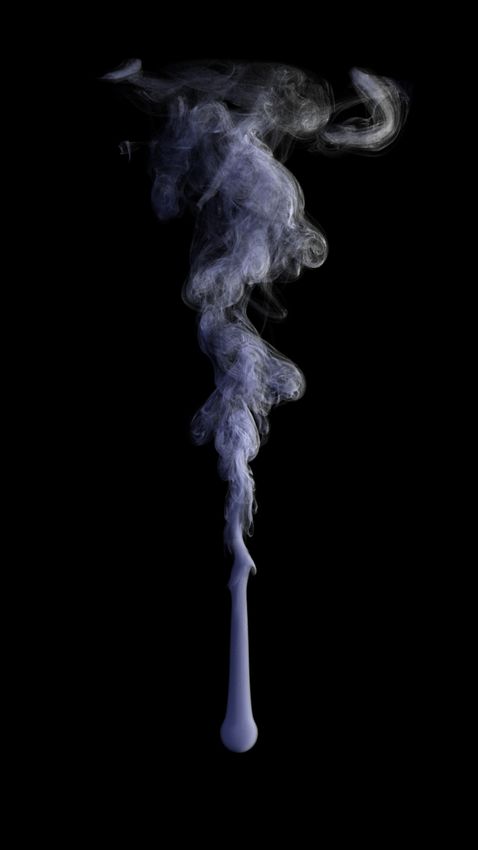
85:8 • J. Zehnder, R. Narain, and B. Thomaszewski

However, when performing this test we noticed that convergence                             Sharif Elcott, Yiying Tong, Eva Kanso, Peter Schröder, and Mathieu Desbrun. 2007.
appears to be improved to second order by performing the second                               Stable, Circulation-preserving, Simplicial Fluids. ACM Trans. Graph. 26, 1 (Jan. 2007).
                                                                                              https://doi.org/10.1145/1189762.1189766
advection half-step using an “extrapolated” velocity field 2u1/2 − u0 ,                    Ronald Fedkiw, Jos Stam, and Henrik Wann Jensen. 2001. Visual Simulation of Smoke.
as a first-order approximation of u1 . We leave a detailed investiga-                         In Proceedings of the 28th Annual Conference on Computer Graphics and Interactive
                                                                                              Techniques (SIGGRAPH ’01). 15–22. https://doi.org/10.1145/383259.383260
tion of this effect to future work.                                                        Nick Foster and Dimitri Metaxas. 1996. Realistic Animation of Liquids. Graphical
                                                                                              Models and Image Processing 58, 5 (Sept. 1996), 471 – 483. https://doi.org/10.1006/
5     CONCLUSIONS                                                                             gmip.1996.0039
                                                                                           Rony Goldenthal, David Harmon, Raanan Fattal, Michel Bercovier, and Eitan Grinspun.
We presented a new method for detail-preserving fluid animation                               2007. Efficient Simulation of Inextensible Cloth. ACM Trans. Graph. 26, 3 (July 2007).
that improves on current advection-projection solver: it replaces the                         https://doi.org/10.1145/1276377.1276438
                                                                                           Ernst Hairer, Christian Lubich, and Gerhard Wanner. 2006. Geometric Numerical
energy-dissipating projection applied at the end of a simulation step                         Integration: Structure-Preserving Algorithms for Ordinary Differential Equations; 2nd
with an energy-preserving reflection in the middle of the interval.                           ed. Springer, Dordrecht. https://cds.cern.ch/record/1250576
                                                                                           Francis H. Harlow and J. Eddie Welch. 1965. Numerical Calculation of Time-Dependent
   Compared to existing advection-projection methods, the central                             Viscous Incompressible Flow of Fluid with Free Surface. The Physics of Fluids 8, 12
advantages of our reflection solver are that i) it has provably bet-                          (1965), 2182–2189. https://doi.org/10.1063/1.1761178
ter energy-conservation properties, and ii) it empirically leads to                        Markus Ihmsen, Jens Orthmann, Barbara Solenthaler, Andreas Kolb, and Matthias
                                                                                              Teschner. 2014. SPH Fluids in Computer Graphics. In Eurographics 2014 - State of
much less vorticity diffusion and preserves more detail for equal                             the Art Reports. https://doi.org/10.2312/egst.20141034
computational costs. Furthermore, our method integrates readily                            Geoffrey Irving, Craig Schroeder, and Ronald Fedkiw. 2007. Volume Conserving Finite
with existing grid-based solvers and is very easy to implement.                               Element Simulations of Deformable Models. ACM Trans. Graph. 26, 3 (July 2007).
                                                                                              https://doi.org/10.1145/1276377.1276394
                                                                                           Chenfanfu Jiang, Craig Schroeder, Andrew Selle, Joseph Teran, and Alexey Stomakhin.
5.1    Limitations & Future Work                                                              2015. The affine particle-in-cell method. ACM Transactions on Graphics (TOG) 34, 4
                                                                                              (July 2015), 51:1–51:10. https://doi.org/10.1145/2766996
While our reflection solver preserves energy and vorticity very well,                      ByungMoon Kim, Yingjie Liu, Ignacio Llamas, and Jarek Rossignac. 2005. FlowFixer: Us-
it does not do so perfectly. One reason is that the semi-Lagrangian                           ing BFECC for Fluid Simulation. In Proceedings of the First Eurographics Conference on
                                                                                              Natural Phenomena (NPH’05). 51–56. https://doi.org/10.2312/NPH/NPH05/051-056
advection step is itself not energy-preserving. Another one is that                        ByungMoon Kim, Yingjie Liu, Ignacio Llamas, and Jarek Rossignac. 2007. Advections
the projection at the end still removes energy from the system, albeit                        with Significantly Reduced Dissipation and Diffusion. IEEE Transactions on Visual-
at a much smaller rate than current advection-projection solvers.                             ization and Computer Graphics 13, 1 (Jan. 2007), 135–144. https://doi.org/10.1109/
                                                                                              TVCG.2007.3
   While the improved energy and vorticity behavior generally lead                         Doyub Kim, Oh-young Song, and Hyeong-Seok Ko. 2008a. A Semi-Lagrangian CIP
to visually richer animations, our solver does not introduce detail                           Fluid Solver without Dimensional Splitting. Computer Graphics Forum 27, 2 (April
where none should arise according to the true solution. In visual                             2008), 467–475. https://doi.org/10.1111/j.1467-8659.2008.01144.x
                                                                                           Theodore Kim, Nils Thürey, Doug James, and Markus Gross. 2008b. Wavelet Turbulence
effects, however, it is often desirable to artificially enhance results,                      for Fluid Simulation. ACM Trans. Graph. 27, 3 (Aug. 2008), 50:1–50:6. https://doi.
e.g., by amplifying vorticity or injecting turbulence. Our solver                             org/10.1145/1360612.1360649
                                                                                           B.P. Leonard. 1979. A stable and accurate convective modelling procedure based on
can, in principle, be used on conjunction with such methods and                               quadratic upstream interpolation. Computer Methods in Applied Mechanics and
it would be interesting to investigate its behavior in this context.                          Engineering 19, 1 (1979), 59 – 98. https://doi.org/10.1016/0045-7825(79)90034-3
Furthermore, we also like to combine our reflection solver with                            Jeroen Molemaker, Jonathan M. Cohen, Sanjit Patel, and Junyong Noh. 2008. Low
                                                                                              Viscosity Flow Simulations for Animation. In SCA ’08: Proceedings of the 2007 ACM
the recent advection-enhancing methods of Zhang et al. [2015] and                             SIGGRAPH/Eurographics Symposium on Computer Animation. 9–18. https://doi.org/
Chern et al. [2016].                                                                          10.2312/SCA/SCA08/009-018
   Extensions to simplicial grids are another direction worth explor-                      Patrick Mullen, Keenan Crane, Dmitry Pavlov, Yiying Tong, and Mathieu Desbrun.
                                                                                              2009. Energy-preserving Integrators for Fluid Animation. ACM Trans. Graph. 28, 3
ing. Finally, we would like to apply the reflection solver to other                           (July 2009), 38:1–38:8. https://doi.org/10.1145/1531326.1531344
constraint-projection applications such as inextensible cloth [Gold-                       Sang Il Park and Myoung Jun Kim. 2005. Vortex Fluid for Gaseous Phenomena. In
                                                                                              Proceedings of the 2005 ACM SIGGRAPH/Eurographics Symposium on Computer
enthal et al. 2007] and volume-preserving solids [Irving et al. 2007]                         Animation (SCA ’05). 261–270. https://doi.org/10.1145/1073368.1073406
that have so far relied on the step-and-project approach.                                  André Robert. 1981. A stable numerical integration scheme for the primitive meteoro-
                                                                                              logical equations. Atmosphere-Ocean 19, 1 (1981), 35–46. https://doi.org/10.1080/
ACKNOWLEDGMENTS
                                                                                              07055900.1981.9649098
                                                                                           Andrew Selle, Ronald Fedkiw, Byungmoon Kim, Yingjie Liu, and Jarek Rossignac. 2008.
We thank the anonymous reviewers for their constructive and                                   An Unconditionally Stable MacCormack Method. J. Sci. Comput. 35, 2-3 (June 2008),
                                                                                              350–371. https://doi.org/10.1007/s10915-007-9166-4
thoughtful feedback. This work was supported by the Discovery                              Andrew Selle, Nick Rasmussen, and Ronald Fedkiw. 2005. A vortex particle method
Grants Program of the Natural Sciences and Engineering Research                               for smoke, water and explosions. ACM Transactions on Graphics (TOG) 24, 3 (July
                                                                                              2005), 910–914. https://doi.org/10.1145/1073204.1073282
Council of Canada (NSERC).                                                                 Jos Stam. 1999. Stable fluids. In Proceedings of the 26th annual conference on Computer
                                                                                              graphics and interactive techniques. 121–128. https://doi.org/10.1145/311535.311548
REFERENCES                                                                                 Nils Thuerey, Theodore Kim, and Tobias Pfaff. 2013. Turbulent fluids. In ACM SIGGRAPH
                                                                                              2013 Courses. ACM, 6.
Alexis Angelidis and Fabrice Neyret. 2005. Simulation of Smoke Based on Vortex Fila-
                                                                                           Nils Thuerey and Tobias Pfaff. 2016. Mantaflow. http://mantaflow.com. (2016).
   ment Primitives. In Proceedings of the 2005 ACM SIGGRAPH/Eurographics Symposium
                                                                                           Steffen Weißmann and Ulrich Pinkall. 2010. Filament-based Smoke with Vortex Shed-
   on Computer Animation (SCA ’05). 87–96. https://doi.org/10.1145/1073368.1073380
                                                                                              ding and Variational Reconnection. ACM Trans. Graph. 29, 4 (July 2010), 115:1–115:12.
Christopher Batty, Florence Bertails, and Robert Bridson. 2007. A Fast Variational
                                                                                              https://doi.org/10.1145/1778765.1778852
   Framework for Accurate Solid-fluid Coupling. ACM Trans. Graph. 26, 3 (July 2007).
                                                                                           Xinxin Zhang, Robert Bridson, and Chen Greif. 2015. Restoring the Missing Vorticity in
   https://doi.org/10.1145/1276377.1276502
                                                                                              Advection-projection Fluid Solvers. ACM Trans. Graph. 34, 4 (July 2015), 52:1–52:8.
Albert Chern, Felix Knöppel, Ulrich Pinkall, Peter Schröder, and Steffen Weißmann.
                                                                                              https://doi.org/10.1145/2766982
   2016. Schrödinger’s Smoke. ACM Trans. Graph. 35, 4 (July 2016), 77:1–77:13. https:
                                                                                           Yongning Zhu and Robert Bridson. 2005. Animating Sand as a Fluid. 24 (July 2005),
   //doi.org/10.1145/2897824.2925868
                                                                                              965–972. https://doi.org/10.1145/1073204.1073298
Alexandre Joel Chorin. 1968. Numerical solution of the Navier-Stokes equations. Math.
   Comp. 22 (1968), 745–762. https://doi.org/10.1090/S0025-5718-1968-0242392-2

ACM Transactions on Graphics, Vol. 37, No. 4, Article 85. Publication date: August 2018.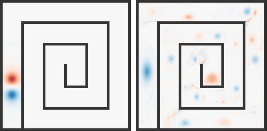
You can also read


