An Efficient Solution to the Five-Point Relative Pose Problem
←
→
Page content transcription
If your browser does not render page correctly, please read the page content below

An Efficient Solution to the Five-Point Relative Pose Problem

                                                                                            David Nistér
                                                                                        Sarnoff Corporation
                                                                                     CN5300, Princeton, NJ 08530
                                                                                        dnister@sarnoff.com

                                            Abstract                                                                  matrix is built, which is subsequently reduced using linear
                                                                                                                      algebra to a 20 × 20 non-symmetric matrix whose eigenval-
An efficient algorithmic solution to the classical five-point                                                         ues and eigenvectors encode the solution to the problem. In
relative pose problem is presented. The problem is to find                                                            [21] an efficient derivation is given that leads to a thirteenth
the possible solutions for relative camera motion between                                                             degree polynomial whose roots include the solutions to the
two calibrated views given five corresponding points. The                                                             five-point problem. The solution presented in this paper is
algorithm consists of computing the coefficients of a tenth                                                           a refinement of this. A better elimination that leads directly
degree polynomial and subsequently finding its roots. It is                                                           in closed form to the tenth degree polynomial is used. Thus,
the first algorithm well suited for numerical implementation                                                          an efficient algorithm that corresponds exactly to the intrin-
that also corresponds to the inherent complexity of the prob-                                                         sic degree of difficulty of the problem is obtained.
lem. The algorithm is used in a robust hypothesise-and-test                                                               For the structure and motion estimation to be robust and
framework to estimate structure and motion in real-time.                                                              accurate in practice, more than five points have to be used.
                                                                                                                      The classical way of making use of many points is to min-
1. Introduction                                                                                                       imise a least squares measure over all points, see for exam-
Reconstruction of camera positions and scene structure                                                                ple [13]. Our intended application for the five-point algo-
based on images of scene features from multiple viewpoints                                                            rithm is as a hypothesis generator within a random sample
has been studied for over two centuries, first by the pho-                                                            consensus scheme (RANSAC) [6]. Many random samples
togrammetry community and more recently in computer vi-                                                               containing five point correspondences are taken. Each sam-
sion. In the classical setting, the intrinsic parameters of the                                                       ple yields a number of hypotheses for the relative orienta-
camera, such as focal length, are assumed known a pri-                                                                tion that are scored by a robust statistical measure over all
ori. This calibrated setting is where the five-point prob-                                                            points in two or more views. The best hypothesis is then
lem arises. Given the images of five unknown scene points                                                             refined iteratively. Such a hypothesise-and-test architecture
from two distinct unknown viewpoints, what are the possi-                                                             has become the standard way of dealing with mismatched
ble solutions for the configuration of the points and cam-                                                            point correspondences [26, 31, 10, 18] and has made auto-
eras? Clearly, only the relative positions of the points and                                                          matic reconstructions spanning hundreds of views possible
cameras can be recovered. Moreover, the overall scale of                                                              [1, 22, 19].
the configuration can never be recovered solely from im-                                                                  The requirement of prior intrinsic calibration was re-
ages. Apart from this ambiguity, the five-point problem was                                                           laxed in the last decade [4, 9, 10], leading to higher flexibil-
proven by Kruppa [14] to have at most eleven solutions.                                                               ity and less complicated algorithms. So, why consider the
This was later improved upon [2, 3, 5, 16, 11], showing that                                                          calibrated setting? Apart from the theoretical interest, one
there are at most ten solutions and that there are ten solu-                                                          answer to this question concerns stability and uniqueness
tions in general (including complex ones). The ten solutions                                                          of solutions. Enforcing the intrinsic calibration constraints
correspond to the roots of a tenth degree polynomial. How-                                                            often gives a crucial improvement of both the accuracy and
ever, Kruppa’s method requires the non-trivial operation of                                                           robustness of the structure and motion estimates. Currently,
finding all intersections between two sextic curves and there                                                         the standard way of achieving this is through an initial un-
is no previously known practical method of deriving the                                                               calibrated estimate followed by iterative refinement to bring
coefficients of the tenth degree polynomial in the general                                                            the estimate into agreement with the calibration constraints.
case. A few algorithms suitable for numerical implemen-                                                               When the intrinsic parameters are known a priori, the five-
tation have also been devised. In [28] a 60 × 60 sparse                                                               point algorithm is a more direct way of enforcing the cal-
                                                                                                                      ibration constraints exactly and obtaining a Euclidean re-
       Prepared through collaborative participation in the Robotics Consortium sponsored by the U. S. Army Research
Laboratory under the Collaborative Technology Alliance Program, Cooperative Agreement DAAD19-01-2-0012. The           construction. The accuracy and robustness improvements
U. S. Government is authorized to reproduce and distribute reprints for Government purposes notwithstanding any
copyright notation thereon.                                                                                           gained by enforcing the calibration constraints are particu-
larly significant for planar or near planar scenes and scenes where the matrix E ≡ [t] × R is called the essential ma-
that appear planar in the imagery. The uncalibrated meth- trix. Any rank-2 matrix is a possible fundamental matrix.
ods fail when faced with coplanar scene points, since there An essential matrix has the additional property that the two
is then a continuum of possible solutions. It has been pro- non-zero singular values are equal. This leads to the fol-
posed to deal with this degeneracy using model selection lowing important cubic constraints on the essential matrix,
[27, 23], switching between a homographic model and the adapted from [25, 5, 16, 21]:
general uncalibrated model as appropriate. In the calibrated Theorem 1 A real non-zero 3 × 3 matrix E is an essential
setting, coplanar scene points only cause at most a two-fold matrix if and only if it satisfies the equation
ambiguity [15, 17]. With a third view, the ambiguity is in 1
general resolved. In light of this, a RANSAC scheme that EE E − trace(EE )E = 0. (5)
2
uses the five-point algorithm over three or more views is
proposed. It applies to general structure but also continues This property will help us recover the essential matrix.
to operate correctly despite scene planarity, without rely- Once the essential matrix is known, R, t and the camera
ing on or explicitly detecting the degeneracy. In essence, matrices can be recovered from it.
the calibrated model can cover both the planar and general
structure cases seamlessly. This gives some hope of deal- 3. The Five-Point Algorithm
ing with the approximately planar cases, where neither the In this section the five-point algorithm is described, first in a
planar nor the uncalibrated general structure model applies straightforward manner. Recommendations for an efficient
well. implementation are then given in Section 3.2. Each of the
The rest of the paper is organised as follows. Section five point correspondences gives rise to a constraint of the
2 establishes some notation and describes the constraints form (4). This constraint can also be written as
used in the calibrated case. Section 3 presents the five-point
algorithm. Section 4 discusses planar degeneracy. Section q̃ Ẽ = 0, (6)
5 outlines the RANSAC schemes for two and three views. where
Section 6 gives results and Section 7 concludes.
q̃≡ q1 q1 q2 q1 q3 q1 q1 q2 q2 q2 q3 q2 q1 q3 q2 q3 q3 q3 (7)
2. Preliminaries and Notation Ẽ≡ E11 E12 E13 E21 E22 E23 E31 E32 E33 (8)
Image points are represented by homogeneous 3-vectors q
By stacking the vectors q̃ for all five points, a 5 × 9 matrix
and q in the first and second view, respectively. World
is obtained. Four vectors X̃, Ỹ , Z̃, W̃ that span the right
points are represented by homogeneous 4-vectors Q. A per-
nullspace of this matrix are now computed. The most com-
spective view is represented by a 3 × 4 camera matrix P
mon way to achieve this is by singular value decomposi-
indicating the image projection q ∼ P Q, where ∼ denotes
tion [24], but QR-factorisation as described in Section 3.2
equality up to scale. A view with a finite projection centre
is much more efficient. The four vectors correspond directly
can be factored into P = K [R | t], where K is a 3 × 3
to four 3 × 3 matrices X, Y, Z, W and the essential matrix
upper triangular calibration matrix holding the intrinsic pa-
must be of the form
rameters and R is a rotation matrix. Let the camera matrices
for the two views be K 1 [I | 0] and P = K2 [R | t]. Let [t]× E = xX + yY + zZ + wW (9)
denote the skew symmetric matrix for some scalars x, y, z, w. The four scalars are only
0 −t3 t2 defined up to a common scale factor and it is therefore
[t]× = t3 0 −t1 (1) assumed that w = 1. Note here that the algorithm can
−t2 t1 0 be extended to using more than 5 points in much the
same way as the uncalibrated 7 and 8-point methods.
so that [t]× x = t×x for all x. Then the fundamental matrix In the overdetermined case, the four singular vectors
is
F ≡ K2− [t]× RK1−1 . (2) X, Y, Z, W that correspond to the four smallest singular
values are used. By inserting (9) into the nine cubic
The fundamental matrix encodes the well known copla-
constraints (5) and performing Gauss-Jordan elimina-
narity, or epipolar constraint
tion with partial pivoting we obtain the equation system
q F q = 0. (3) A x3 y3 x2 y xy2 x2 z y2 z x2 y2 xyz xy xz 2 xz x yz 2 yz y 1
(a) 1 . . . . . . . . . . . . . . . [3]
If K1 and K2 are known, the cameras are said to be cali- (b) 1 . . . . . . . . . . . . . . [3]
(c) 1 . . . . . . . [3]
brated. In this case, we can always assume that the image (d) 1 . . . . . . . [3]
points q and q have been premultiplied by K 1−1 and K2−1 , (e) 1 . . . . . . . [3]
(f ) 1 . . . . . . . [3]
respectively, so that the epipolar constraint simplifies to (g) 1 L . . . M N O [3]
1 P Q R S . . . [3]
q Eq = 0,
(h)
(4) (i) 1 . . . . . . . [3]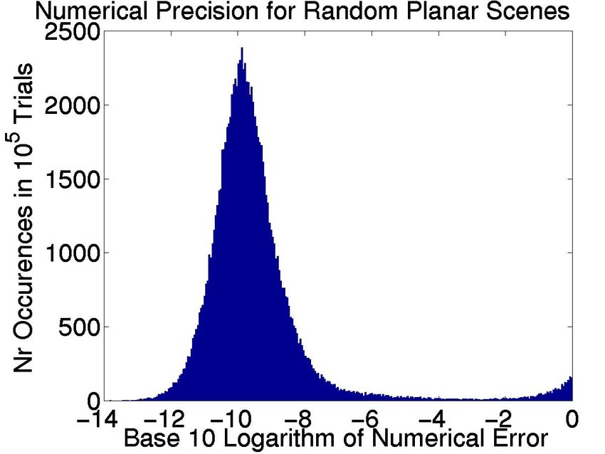
3 × 3 determinants obtained from the first three rows of B
where . and L, . . . , S denote some scalar values and by striking out the columns corresponding to x, y and 1, re-
[n] denotes a polynomial of degree n in the variable z. spectively. The essential matrix is then obtained from (9).
Note that the elimination can optionally be stopped two In Section 3.1 it is described how to recover R and t from
rows early. Further, define the additional equations the essential matrix.
(j) ≡ (e) − z(g) (10)
3.1 Recovering R and t from E
(k) ≡ (f ) − z(h) (11)
(l) ≡ (d) − x(h) + P (c) + zQ(e) + R(e) + S(g) (12) Let
0 1 0
(m) ≡ (c) − y(g) + L(d) + zM (f ) + N (f ) + O(h). (13) D = −1 0 0 . (21)
We now have the five equations 0 0 1
R and t are recovered from the essential matrix on the basis
(i) = xy[1] + x[2] + y[2] + [3] = 0 (14)
of the following theorem [30, 10]:
(j) = xy[1] + x[3] + y[3] + [4] = 0 (15)
(k) = xy[1] + x[3] + y[3] + [4] = 0 (16) Theorem 2 Let the singular value decomposition of the es-
sential matrix be E ∼ U diag(1, 1, 0)V , where U and
(l) = xy[2] + x[3] + y[3] + [4] = 0 (17)
V are chosen such that det(U ) > 0 and det(V ) > 0.
(m) = xy[2] + x[3] + y[3] + [4] = 0. (18)
Then t ∼ tu ≡ u13 u23 u33 and R is equal to
These equations are arranged into two 4 × 4 matrices Ra ≡ U DV or Rb ≡ U D V .
containing polynomials in z: Any combination of R and t according to the above pre-
scription satisfies the epipolar constraint (4). To resolve the
B xy x y 1 C xy x y 1
inherent ambiguities, it is assumed that the first camera ma-
(i) [1] [2] [2] [3] (i) [1] [2] [2] [3]
trix is [I | 0] and that t is of unit length. There are then the
(j) [1] [3] [3] [4] (j) [1] [3] [3] [4]
following four possible solutions for the second camera ma-
(k) [1] [3] [3] [4] (k) [1] [3] [3] [4]
trix: PA ≡ [Ra | tu ], PB ≡ [Ra | −tu ], PC ≡ [Rb | tu ],
(l) [2] [3] [3] [4] (m) [2] [3] [3] [4]
PD ≡ [Rb | −tu ] . One of the four choices corresponds
to the true configuration. Another one corresponds to the
Since the vector [ xy x y 1 ] is a nullvector to twisted pair which is obtained by rotating one of the views
both these matrices, their determinant polynomials must 180 degrees around the baseline. The remaining two corre-
both vanish. Let the two eleventh degree determinant spond to reflections of the true configuration and the twisted
polynomials be denoted by (n) and (o) , respectively. The pair. For example, P A gives one configuration. P C corre-
eleventh degree term is cancelled between them to yield the sponds to its twisted pair, which is obtained by applying the
tenth degree polynomial transformation
(p) ≡ (n)o11 − (o)n11 . (19) I 0
Ht ≡ . (22)
−2v13 −2v23 −2v33 −1
The real roots of (p) are now computed. There are various
standard methods to accomplish this. A highly efficient way PB and PD correspond to the reflections obtained by apply-
is to use Sturm-sequences to bracket the roots, followed by ing Hr ≡ diag(1, 1, 1, −1). In order to determine which
a root-polishing scheme. This is described in Section 3.2. choice corresponds to the true configuration, the cheirality
Another method, which is easy to implement with most lin- constraint 1 is imposed. One point is sufficient to resolve
ear algebra packages, is to eigen-decompose a companion the ambiguity. The point is triangulated using the view pair
matrix. After normalising (p) so that p 10 = 1, the roots are ([I | 0] , PA ) to yield the space point Q and cheirality is
found as the eigenvalues of the 10 × 10 companion matrix tested. If c1 ≡ Q3 Q4 < 0, the point is behind the first
camera. If c2 ≡ (PA Q)3 Q4 < 0, the point is behind the
p9 p8 · · · p0
−1 second camera. If c 1 > 0 and c2 > 0, PA and Q corre-
spond to the true configuration. If c 1 < 0 and c2 < 0, the
.. . (20)
. reflection Hr is applied and we get P B . If on the other hand
−1 c1 c2 < 0, the twist Ht is applied and we get P C and the
point Ht Q. In this case, if Q3 (Ht Q)4 > 0 we are done.
For each root z the variables x and y can be found using
Otherwise, the reflection H r is applied and we get P D .
equation system B. The last three coordinates of a nullvec-
tor to B are computed, for example by evaluating the three 1 The constraint that the scene points should be in front of the cameras.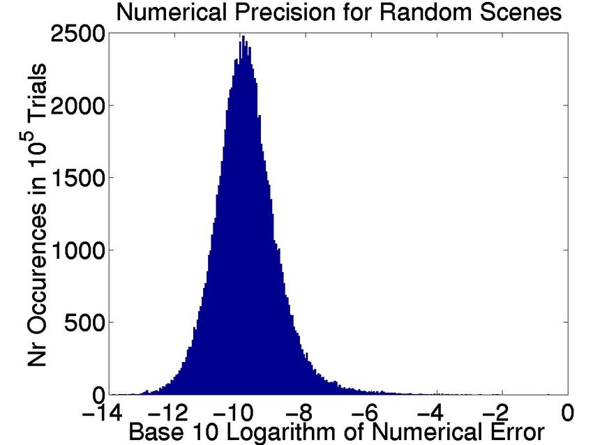
3.2 Efficiency Considerations                                        portion of the computation time, since they have to be car-
                                                                     ried out for each real root. A specifically tailored singular
In summary, the main computational steps of the algorithm            value decomposition is given in Appendix B. Efficient tri-
outlined above are as follows:                                       angulation is discussed in Appendix C. Note that a triangu-
  1. Extraction of the nullspace of a 5 × 9 matrix.                  lation scheme that assumes ideal point correspondences can
                                                                     be used since for true solutions the recovered essential ma-
  2. Expansion of the cubic constraints (5).                         trix is such that intersection is guaranteed for the five pairs
                                                                     of rays.
  3. Gauss-Jordan elimination on the 9 × 20 matrix A.

  4. Expansion of the determinant polynomials of the two             4. Planar Structure Degeneracy
     4 × 4 polynomial matrices B and C followed by elim-
                                                                     The planar structure degeneracy is an interesting example
     ination to obtain the tenth degree polynomial (19).
                                                                     of the differences between the calibrated and uncalibrated
  5. Extraction of roots from the tenth degree polynomial.           frameworks. The degrees of ambiguity that arise from a
                                                                     planar scene in the two frameworks are summarised in Ta-
  6. Recovery of R and t corresponding to each real root             ble 1. For pose estimation with known intrinsics there is a
     and point triangulation for disambiguation.                     unique solution provided that the plane is finite and that the
                                                                     cheirality constraint is taken into account 2 . In theory, focal
We will discuss efficient implementation of Steps 1,5 and            length can also be determined if the principal direction does
6. Singular value decomposition is the gold standard for             not coincide with the plane normal. Without knowledge of
the nullspace extraction in Step 1, but a specifically tailored      the intrinsics however, there is a three degree of freedom
QR-factorisation is much more efficient. The five input vec-         ambiguity that can be thought of as parameterised by the
tors are orthogonalised first, while pivoting, to form the or-       position of the camera centre. For any camera centre, ap-
thogonal basis q̃1 , . . . , q̃5 . This basis is then amended with   propriate choices for the calibration matrix K and rotation
the 9 × 9 identity matrix to form the matrix                         matrix R can together produce any homography between
                                                                  the plane and the image. With known intrinsics and two
                        q̃1   · · · q̃5 | I                  (23)    views of an unknown plane, there are two solutions for the
                                                                     essential matrix [15, 17], unless the baseline is perpendic-
The orthogonalisation with pivoting is now continued until           ular to the plane in which case there is a unique solution.
nine orthogonal vectors are obtained. The last four rows             The cheirality constraint resolves the ambiguity unless all
constitute an orthogonal basis for the nullspace.                    visible points are closer to one viewpoint than the other
    Sturm sequences are used to bracket the roots in Step 5.         [15]. If all visible points are closer to one viewpoint, the
The definition of a Sturm sequence, also called Sturm chain          dual solution is obtained from the true one by reflecting that
is given in Appendix A. The tenth degree polynomial has an           view across the plane and then taking the twisted pair of
associated Sturm sequence, which consists of eleven poly-            the resulting configuration. Any attempts to recover intrin-
nomials of degree zero to ten. The number of real roots in an        sic parameters from two views of a planar surface are futile
interval can be determined by counting the number of sign            according to the following theorem, adapted from [16]:
changes in the Sturm sequence at the two endpoints of the
interval. The Sturm sequence can be evaluated recursively            Theorem 3 For any choice of intrinsic parameters, any ho-
with 38 floating point operations. 10 additional operations          mography can be realised between two views by some posi-
are required to count the number of sign changes. This is to         tioning of the two views and a plane.
be put in relation to the 20 floating point operations required
to evaluate the polynomial itself. With this simple test for         If the calibration matrices are completely unknown, there is
number of roots in an interval, it is fairly straightforward         a two degree of freedom ambiguity, that can be thought of
to hunt down a number of intervals, each containing one of           as parameterised by the epipole in one of the images, i.e.
the real roots of the polynomial. Any root polishing scheme          for any choice of epipole in the first image, there is a unique
[24] can then be used to determine the roots accurately. In          valid solution. Once the epipole is specified in the first im-
our experiments we simply use 30 iterations of bisection,            age, the problem of solving for the remaining parameters of
since this provides a guaranteed precision in fixed time and         the fundamental matrix is algebraically equivalent to solv-
requires almost no control overhead.                                 ing for the projective pose of a one-dimensional camera in
    Step 6 requires a singular value decomposition of the            a two-dimensional world, where the projection centre of the
essential matrix and triangulation of one or more points.               2 If the plane is the plane at infinity it is impossible to determine the
When all the other steps of the algorithm have been effi-            camera position and without the cheirality constraint the reflection across
ciently implemented, these operations can take a significant         the plane constitutes a second solution.
1 View Known 2 Views Un- n > 2 Views
Structure known Struc- Unknown
6. Results
ture Structure
Known intrin- Unique Two-fold or Unique For a minimal solution such as the five-point method the
sics unique
Unknown fixed Unique in gen- 1 d.o.f. Unique in gen- two main requirements are precision and speed. Observe
focal length eral eral that the effects of noise will be the same for any five-point
Unknown vari- 3 d.o.f. 2 d.o.f. 3n-4 d.o.f.
able intrinsics solution method. The numerical precision of our fast imple-
Table 1: The degrees of ambiguity in the face of planar degener- mentation is investigated in Figure 1. Note that the typical
acy for pose estimation and structure and motion estimation. The errors are insignificant in comparison to realistic noise lev-
motion is assumed to be general and the structure is assumed to be els.
dense in the plane. See the text for further explanation. The computation time is partially dependent on the num-
1-D camera corresponds to the epipole in the second image, ber of real solutions. The distribution of the number of so-
the orientation corresponds to the epipolar line homogra- lutions is given in Table 2. We have also verified experi-
phy and the points in the second image correspond to world mentally that five points in three views in general yield a
points in the 2-D space. The problem according to Chasles’ unique solution, with or without planar structure and an un-
Theorem [10] has a unique solution unless all the points known focal length common to the three views. Timing in-
and the epipole in the second image lie on a conic, which formation for our efficient implementation of the five-point
is not the case since we are assuming that the structure is algorithm is given in Table 3.
dense in the plane. For three views with known intrinsics The algorithm is used as a part of a system that recon-
there is a unique solution. If the views are in general posi- structs structure and motion from video in real-time. Sys-
tion a common unknown focal length can also be recovered, tem timing information is given in Table 4. Some results
but this requires rotation and suffers from additional critical from the reconstruction system are given in Figures 2-6. See
configurations. With unknown variable intrinsics there are the figure captions for details.
3 additional degrees of freedom for each view above two.
5. Applying the Algorithm Together
with Random Sample Consensus
We use the algorithm in conjunction with random sampling
consensus in two or three views. A number of random sam-
ples are taken, each containing five point-tracks. The five-
point algorithm is applied to each sample and thus a number
of hypotheses are generated. In the two-view case, the hy- Figure 1: Distribution of the numerical error in the computed
potheses are scored by a robust measure over all the point essential matrix Ê based on 105 random tests with generic (left)
pairs and the hypothesis with the best score is retained. Fi- and planar (right) scenes. Since the matrix is up to scale and there
nally, the best hypothesis can be polished by iterative refine- are multiple solutions Êi , the minimum residual
ment [29]. When three or more views are available, we pre- min min( Ê i
Ê
E
− E E
, E + Ê i
Ê
) from each problem
i i i
fer to disambiguate and score the hypotheses utilising three instance is used. The median error is 1.39 · 10−10 for generic
views. A unique solution can then be obtained from each scenes and 1.76 · 10−10 for planar scenes. All computations were
sample of five tracks and this continues to hold true even if performed in double precision.
the scene points are all perfectly coplanar. For each sam-
ple of five point-tracks, the points in the first and last view
are used in the five-point algorithm to determine a number 7. Summary and Conclusions
of possible camera matrices for the first and last view. For
each case, the five points are triangulated 3 . The remaining An efficient algorithm for solving the five-point relative
view can now be determined by any 3-point calibrated per- pose problem was presented. The algorithm was used in
spective pose algorithm, see [8] for a review and additional conjunction with random sampling consensus to solve for
references. Up to four solutions are obtained and disam- unknown structure and motion over two, three or more
biguated by the additional two points. The reprojection er- views. The efficiency of the algorithm is very impor-
rors of the five points in all of the views are now enough to tant since it will typically be applied within this kind of
single out one hypothesis per sample. Finally, the solutions hypothesise-and-test architecture, where the algorithm is
from all samples are scored by a robust measure using all executed for hundreds of different five-point samples. Prac-
available point tracks. tical real-time reconstruction results were given and it was
shown that the calibrated framework can continue to oper-
3 See Appendix C. ate correctly despite scene planarity.Nr Hyp 0 1 2 3 4 5 6 7
10 8 9 Matching with Disparity Range
Feature Detection SaM
Step 5 0 . 0.12 . 0.50 . 0.36 .
4.9e 0.15 . 3% 5% 10%
30ms 50ms
−4 34ms 45ms 160ms
Step 6 4.2e 0.17 0.28 0.29 0.17 5.8e 2.5e 1.5e 6.6e 1.5e 2e
−6 −2 −2 −3 −4 −6 −7 Table 4: Approximate average timings per 720x240 frame of
video for the system components on a modest 550MHz machine.
Table 2: The distribution of the number of hypotheses that result
MMX code was used for the crucial parts of the feature detection
from computational steps 5 and 6 (as numbered in Section 3.2).
and feature matching. Disparity range for the matching is given
The second row shows the distribution of the number of real roots
in percent of the image dimensions. In the structure and motion
of the tenth degree polynomial (p) in Equation (19), based on 105
component (SaM), one-view and three-view estimations are com-
random point and view configurations. The average is 4.55 roots.
bined to incrementally build the reconstruction with low latency.
The third row shows the distribution of the number of hypothe-
The whole system including all overhead currently operates at 26
ses once the cheirality constraint has been enforced, based on 107
frames per second on average on a 2.4GHz machine when using
random point and view configurations. The average number of hy-
a 3% disparity range. The latency is also small, since there is no
potheses is 2.74. Both rows show fractions of the total number of
self-calibration and only very local iterative refinements.
trials. Our current randomization leads to two cases in 107 with
ten distinct physically valid solutions. We have verified that there
are such cases with ten well separated solutions that are not caused
by numerical inaccuracies.
Step 1 2 3 4 5 6 Three- Mean Mean
Point Two Three
Pose Views Views
µs 8 12 23 14 6/root 8/root 5/root 121 134
Table 3: Approximate timings for the algorithm steps (as num-
bered in Section 3.2) on a modest 550MHz machine with highly
optimised but platform-independent code. Including all overhead,
the two and three view functions typically take 110-140µs and
120-180µs, respectively. For RANSAC processes with 500 sam- Figure 2: Reconstruction from the turntable sequence ’Stone’.
ples the total hypothesis generation times are around 60ms and No prior knowledge about the motion or the fact that it closes on
67ms, respectively. itself was used in the estimation. The circular shape of the es-
timated trajectory is a verification of the correctness of the result.
This result was obtained without any global bundle adjustment and
Appendixes exhibits a regularity and accuracy that is typically not obtained
with an uncalibrated method until the calibration constraints have
A Definition of Sturm Chain been enforced through bundle adjustment.
Let p(z) be a general polynomial of degree n >= 2. Here,
the significance of general is that we ignore special cases for point z through Equations (26, 27) and the recursion
the sake of brevity. For example, p(z) is assumed to have no
fi (z) = (ki z + mi )fi−1 (z) − fi−2 (z) i = 2, . . . , n (28)
multiple roots. Moreover, the polynomial divisions carried
out below are assumed to have a non-zero remainder. Under
Let the number of sign changes in the chain be s(z). The
these assumptions, the Sturm chain is a sequence of poly-
number of real roots in an interval [a, b] is then s(a) − s(b).
nomials f0 , . . . , fn of degrees 0, . . . , n, respectively. f n is
Unbounded intervals such as for example [0, ∞) can be
the polynomial itself and f n−1 is its derivative:
treated by looking at m 0 and k0 , . . . , kn in order to calculate
fn (z) ≡ p(z) (24) limz→∞ s(z). For more details, see for example [7, 12].
fn−1 (z) ≡ p (z). (25)
For i = n, . . . , 2 we carry out the polynomial division B Efficient Singular Value Decompo-
fi /fi−1 . Let the quotient of this division be q i (z) =
ki z + mi and let the remainder be r i (z), i.e. fi (z) =
sition of the Essential Matrix
qi (z)fi−1 (z) + ri (z). Then define f i−2 (z) ≡ −ri (z). Fi- An efficient singular value decomposition according to the
nally, define the coefficients m 0 , m1 and k1 such that conditions of Theorem 2 is given. Let the essential matrix
f0 (z) = m0 (26) be E = ea eb ec , where ea , eb , ec are column-
f1 (z) = k1 z + m1 . (27) vectors. It is assumed that it is a true essential matrix, i.e.
that it has rank two and two equal non-zero singular values.
Once the scalar coefficients k 1 , . . . , kn and m0 , . . . , mn First, all the vector products e a × eb , ea × ec and eb × ec are
have been derived, the Sturm chain can be evaluated at any computed and the one with the largest magnitude chosen.Figure 5: Reconstruction from the sequence ’Girlsstatue’ that
was acquired with a handheld camera. Only approximate intrin-
Figure 3: Reconstructions obtained from the ’Stone’ sequence sic parameters were used and no global bundle adjustment was
by setting the focal length to incorrect values. The focal lengths performed.
used were 0.05, 0.3, 0.5, 0.7, 1.3, 1.5, 2.0 and 3.0 times the value
obtained from calibration. For too small focal lengths, the recon-
struction ’unfolds’ and vice versa.
Figure 4: Reconstruction from the sequence ’Farmhouse’, which
contains long portions where a single plane fills the field of view.
The successful reconstruction is a strong practical proof of the fact
that the calibrated framework can overcome planar structure de-
generacy without relying on the degeneracy or trying to detect it.
This is especially important for near-planar scenes, where neither
the planar nor the uncalibrated model applies well. Only approx-
imate intrinsic parameters were used and no global bundle adjust-
ment was performed.
Figure 6: Reconstruction from vehicle sequences ’Road’, ’Park-
Assume without loss of generality that e a ×eb has the largest ing Lot’ and ’Turn’, with 360, 330 and 130 frames, respectively.
magnitude. Define v c ≡ (ea × eb )/|ea × eb |, va ≡ ea /|ea |, Only approximate intrinsic parameters were used and no global
vb ≡ vc × va , ua ≡ Eva /|Eva |, ub ≡ Evb /|Evb | and bundle adjustment was performed.
uc ≡ ua × ub. Then the singular
valuedecomposition is
given by V = va vb vc and U = ua ub uc .
polynomial, see [10]. Minimisation of . ∞ -norm [19],
or directional error [20], also yields good results in prac-
tice and can be achieved in closed form an order of mag-
C Efficient Triangulation of an Ideal nitude faster. In the ideal situation, triangulation can be
Point Correspondence accomplished very efficiently by intersecting three planes
that are back-projected from image lines. The image lines
In the situation encountered in the five-point algorithm chosen to generate the three planes are the epipolar line
where triangulation is needed, a hypothesis for the essen- a corresponding to q , the line b through q that is per-
tial matrix E has been recovered and along with it the two pendicular to a and the line c through q that is perpen-
camera matrices [I | 0] and P . No error metric has to be dicular to Eq. For non-ideal point correspondences, this
minimised, since for the true solution the rays backpro- scheme finds the world point on the ray backprojected from
jected from the image correspondence q↔ q are guaran- q that minimises the reprojection error in the first image.
teed to meet. For non-ideal point correspondences, prior It triangulates world points at infinity correctly and is in-
correction to guarantee ray-intersection while minimising a variant to projective transformations of the world space.
good error metric is recommended. Global minimisation Observe that a = E q , b = q × (diag(1, 1, 0)a) and
of . 2 -norm in two views requires solving a sixth degree c = q × (diag(1, 1, 0)Eq). Moreover, A ≡ [ a 0 ]is the plane backprojected from a, B ≡ [ b 0 ] is the [14] E. Kruppa, Zur Ermittlung eines Objektes aus zwei Perspek-
plane backprojected from b and C ≡ P c is the plane back- tiven mit Innerer Orientierung, Sitz.-Ber. Akad. Wiss., Wien,
projected from c. The intersection between the three planes Math. Naturw. Kl., Abt. IIa., 122:1939-1948, 1913.
[15] H. Longuet-Higgins, The Reconstruction of a Plane Surface
A, B and C is now sought. Formally, the intersection is the
from Two Perspective Projections, Proc. R. Soc. Lond. B,
contraction Q l ≡ 7ijkl Ai B j C k between the epsilon tensor 277:399-410, 1986.
7ijkl 4 and the three planes. More concretely, d ≡ a × b [16] S. Maybank, Theory of Reconstruction from Image Motion,
is the direction of the ray backprojected from the intersec- Springer-Verlag, ISBN 3-540-55537-4, 1993.
tion between a and b. The space point is the intersection [17] S. Negahdaripour, Closed-Form Relationship Between the
between this ray and the plane C: Two Interpretations of a Moving Plane, J. Optical Society of
America, 7(2):279-285, 1990.
[18] D. Nistér. Reconstruction From Uncalibrated Sequences
Q ∼ d C4 −(d1 C1 + d2 C2 + d3 C3 ) . (29)
with a Hierarchy of Trifocal Tensors, Proc. European Con-
ference on Computer Vision, Volume 1, pp. 649-663, 2000.
Finally, it is observed that in the particular case of an ideal [19] D. Nistér. Automatic dense reconstruction from uncalibrated
point correspondence we have d = q, so that computing a, b video sequences, PhD Thesis, Royal Institute of Technology
and A, B can be avoided altogether. KTH, ISBN 91-7283-053-0, March 2001.
[20] J. Oliensis and Y. Genc, New Algorithms for Two-Frame
References Structure from Motion, Proc. International Conference on
[1] P. Beardsley, A. Zisserman and D. Murray, Sequential updat- Computer Vision, pp. 737-744 ,1999.
ing of projective and affine structure from motion, Interna- [21] J. Philip, A Non-Iterative Algorithm for Determining all
tional Journal of Computer Vision, 23(3): 235-259, 1997. Essential Matrices Corresponding to Five Point Pairs, Pho-
[2] M. Demazure, Sur Deux Problemes de Reconstruction, Tech- togrammetric Record, 15(88):589-599, October 1996.
nical Report No 882, INRIA, Rocquencourt, France, 1988. [22] M. Pollefeys, R. Koch and L. Van Gool, Self-Calibration and
[3] O. Faugeras and S. Maybank, Motion from Point Matches: Metric Reconstruction in spite of Varying and Unknown In-
Multiplicity of Solutions, International Journal of Computer ternal Camera Parameters, International Journal of Computer
Vision, 4(3):225-246, 1990. Vision, 32(1):7-25, 1999.
[23] M. Pollefeys, F. Verbiest and L. Van Gool, Surviving Dom-
[4] O. Faugeras, What Can be Seen in Three Dimensions with
inant Planes in Uncalibrated Structure and Motion Recovery,
an Uncalibrated Stereo Rig?, Proc. European Conference on
Proc. European Conference on Computer Vision, Volume 2,
Computer Vision, pp. 563-578, 1992.
pp. 837-851, 2002.
[5] O. Faugeras, Three-Dimensional Computer Vision: a Geo-
[24] W. Press, S. Teukolsky, W. Vetterling and B. Flannery, Nu-
metric Viewpoint, MIT Press, ISBN 0-262-06158-9, 1993.
merical recipes in C, Cambridge University Press, ISBN 0-
[6] M. Fischler and R. Bolles, Random Sample Consensus: a
521-43108-5, 1988.
Paradigm for Model Fitting with Application to Image Anal- [25] P. Stefanovic, Relative Orientation - a New Approach, I. T.
ysis and Automated Cartography, Commun. Assoc. Comp. C. Journal, 1973-3:417-448, 1973.
Mach., 24:381-395, 1981. [26] P. Torr and D. Murray, The Development and Comparison of
[7] W. Gellert, K. Küstner, M. Hellwich and H. Kästner, The VNR Robust Methods for Estimating the Fundamental Matrix, In-
Concise Encyclopedia of Mathematics, Van Nostrand Rein- ternational Journal of Computer Vision, 24(3):271-300, 1997.
hold Company, ISBN 0-442-22646-2, 1975. [27] P. Torr, A. Fitzgibbon and A. Zisserman, The Problem of
[8] R. Haralick, C. Lee, K. Ottenberg and M. Nölle, Review and Degeneracy in Structure and Motion Recovery from Uncali-
Analysis of Solutions of the Three Point Perspective Pose Es- brated Image Sequences, International Journal of Computer
timation Problem, International Journal of Computer Vision, Vision, 32(1):27-44, August 1999.
13(3):331-356, 1994. [28] B. Triggs, Routines for Relative Pose of Two Cal-
[9] R. Hartley, Estimation of Relative Camera Positions for Un- ibrated Cameras from 5 Points, Technical Report,
calibrated Cameras, Proc. European Conference on Computer http://www.inrialpes.fr/movi/people/Triggs INRIA, France,
Vision, pp. 579-587, 1992. 2000.
[10] R. Hartley and A. Zisserman, Multiple View Geometry in [29] B. Triggs, P. McLauchlan, R. Hartley and A. Fitzgibbon,
Computer Vision, Cambridge University Press, ISBN 0-521- Bundle Adjustment - a Modern Synthesis, Springer Lecture
62304-9, 2000. Notes on Computer Science, Springer Verlag, 1883:298-375,
[11] A. Heyden and G. Sparr, Reconstruction from Calibrated 2000.
[30] R. Tsai and T. Huang, Uniqueness and Estimation of
Cameras - a New Proof of the Kruppa-Demazure Theorem,
Three-Dimensional Motion Parameters of Rigid Objects with
Journal of Mathematical Imaging & Vision, 10:1-20, 1999.
Curved Surfaces, IEEE Transactions on Pattern Analysis and
[12] D. Hook and P. McAree, Using Sturm Sequences To Bracket
Machine Intelligence, 6(1):13-27, 1984.
Real Roots of Polynomial Equations, Graphic Gems I, Aca- [31] Z. Zhang, Determining the Epipolar Geometry and its Uncer-
demic Press, ISBN 0-122-86166-3, pp. 416-423, 1990. tainty: a Review, International Journal of Computer Vision,
[13] B. Horn, Relative Orientation, International Journal of Com- 27(2):161-195, 1998.
puter Vision, 4:59-78, 1990.
i j k l
ijkl is the tensor such that ijkl A B C D =
4 The epsilon tensor The views and conclusions contained in this document are those of the authors and should not be interpreted as
representing the official policies, either expressed or implied, of the Army Research Laboratory or the U. S. Govern-
det([ A B C D ]). ment.You can also read