An improved bi-objective salp swarm algorithm based on decomposition for green scheduling in exible manufacturing cellular environments with ...

An improved bi-objective salp swarm algorithm
based on decomposition for green scheduling in
 exible manufacturing cellular environments with
multiple automated guided vehicles
Binghai Zhou (  bhzhou@tongji.edu.cn )
 Tongji University School of Mechanical Engineering https://orcid.org/0000-0002-6599-9033
Jihua Zhang
 Tongji University School of Mechanical Engineering

Research Article

Keywords: Flexible manufacturing cell, automated guided vehicle, bi-objective, energy-e ciency, salp
swarm algorithm, stochastic-distribution-based operators

Posted Date: January 24th, 2023

DOI: https://doi.org/10.21203/rs.3.rs-2456083/v1

License:   This work is licensed under a Creative Commons Attribution 4.0 International License.
Read Full License

An improved bi-objective salp swarm algorithm based on
 decomposition for green scheduling in flexible manufacturing cellular
 environments with multiple automated guided vehicles

 Bing-Hai Zhou1*, Ji-Hua Zhang2,

 * Corresponding author

 1 School of Mechanical Engineering, Tongji University, Shanghai 201804, PR China

 Phone: +86 21 69589598

 Fax: +86 21 69589598

 Email: bhzhou@tongji.edu.cn

 2 School of Mechanical Engineering, Tongji University, Shanghai 201804, PR China

 Phone: +86 21 69589598

 Fax: +86 21 69589598

 Email: 2030219@tongji.edu.cn

Abstract:
 Energy-awareness in the industrial sectors has become a global consensus in recent decades. Green
scheduling is acknowledged as an effective weapon to reduce energy consumption in the industrial
sectors. Therefore, this paper is devoted to the green scheduling of flexible manufacturing cells (FMC)
with auto-guided vehicle transportation, where conflict-free routing of the vehicles is considered. To deal
with this problem, a bi-objective optimization model is proposed to achieve the minimization of the
maximum completion time and the total energy consumption in an FMC. The studied problem is an
extension of flexible job shop problem which is NP-hard. Thus, an improved bi-objective salp swarm
algorithm based on decomposition (IMOSSA/D) is proposed and applied to the problem. The approach
is based on the decomposition of the bi-objective problem. Salp swarm intelligence along with three
stochastic-distribution-based operators are incorporated into the approach, to enhance and balance its
exploring and exploiting ability. Computational experiments are performed to compare the proposed
approach with two state-of-the-art algorithms. This study allows the decision makers to better trade-off
between energy savings and production efficiency in flexible manufacturing cellular environment.

Keywords：

Flexible manufacturing cell; automated guided vehicle; bi-objective; energy-efficiency; salp swarm
algorithm; stochastic-distribution-based operators

1. Introduction

 The manufacturing societies are pushed to improve their product suits by rapidly changing customer
needs, especially during the third industrial revolution (from the 1980s to today) (Yin et al. 2018). The
quest for high productivity and low cost is no longer the whole story, while product personalization and
on-time delivery are also emphasized. For this purpose, flexible manufacturing has emerged and is
growing at a rapid pace which can meet customer needs of high variability and customization with higher
flexibility, automation and productivity. It can be implemented in several system configurations, among
which flexible manufacturing cells (FMCs) are dominating and particularly favored by small and
medium-sized enterprises (Ito 2013). Also, flexible manufacturing systems (FMS) often require the
integration of a set of FMCs. FMCs represent not only today's manufacturing industry, but also its future.
The Internet of things, electric vehicles, and artificial intelligence, each of which are playing a role in the
new industrial revolution, are beginning to be incorporated into FMCs. These technologies will further
enhance the strengths of FMCs.
 A typical FMC consists of one or more flexible machines, an automated handling system and a central
control system (Tuysuz and Kahraman 2010). Processing and transportation are the two main activities
of FMCs, which are highly interconnected, making the scheduling of these activities exceedingly
complex. Faced with such difficulties, many shop floor scheduling studies choose to focus on processing
activities rather than handling processes to achieve simplification. Ignoring the transportation processes,
the scheduling of FMC can be simplified as the flexible job shop scheduling problem (FJSSP), an
relaxation of the job shop problem (Jurisch 1995). FJSSP is a scheduling problem with important
applications and has been widely studied (Deliktas et al. 2021). FJSSPs of their basic version do not
involve any transportation process. However, in recent years, more and more researchers have started to
emphasize the importance of material handling in shop floor scheduling problems. For example, there
are studies on FJSSPs considering transport time (Wang et al. 2021), transportation costs (Ziaee et al.
2022), crane handling (Zhou and Liao 2020), etc. Extensive review on FJSSPs has been done by Gao et
al. (2019).
 As for transportation in an FMC, it is generally achieved by tools such as conveyors, cranes, and

automated guided vehicles（AGV）, which can be incorporated into the scheduling model, making the

model more realistic. Among these transporting tools, AGVs have been more and more used due to their
flexibility, energy-efficiency and cost advantage (Bechtsis et al. 2017). Although material handling with
AGV in manufacturing systems is a hot topic in the literature, most studies assume that the path of the
AGV is known or the number of the AGVs is unlimited, which is far from the case in reality. For example,
Fontes and Homayouni (2019) studied joint production and AGV transport scheduling in flexible
manufacturing systems, but with pre-determined travel time between machines. Zhao et al. (2020)
designed and implemented a multi-AGV scheduling approach for a job shop, where the AGVs are
navigated by magnetic strips. (He et al. 2022)studied an energy-efficient multi-objective production
scheduling problem, with which integrated with multiple AGVs with pre-determined routes.

However, the scheduling problem associated with AGVs can be even more complex and closer to
real-world production systems if more realistic factors such as vehicle routing, conflict avoidance and
battery depletion can be taken into account. Due to its high complexity, too few works have been done
so far on conflict-free routing of AGVs in FMCs. Therefore, this paper takes this into consideration,
which may bridge some of the gaps between the existing research and the real-world implementations.
 The diversity of scheduling criteria needs to be improved in addition to the consideration of the
transportation issue in an FMC. Energy efficiency has gradually become another compelling issue
nowadays, while operational criteria, such as make span, have been the most focused criterions of shop
floor scheduling, (Gao et al. 2020). Reducing energy consumption and greenhouse gas emissions has
received widespread attention in manufacturing industry and academia, as global warming and the energy
crisis have intensified over the decades (Diaz and Ocampo-Martinez 2019). Due to this reason, green
scheduling, also often referred to as energy-efficient scheduling, has been rising as an effective means to
promote energy-efficiency in the industrial sector. Green scheduling tries to achieve energy saving
through scientific planning of activities in the manufacturing systems, in this case, FMCs. For example,
Zhou and Zhu (2021b) worked on multi-objective greening scheduling optimization of part feeding for
mixed model assembly lines with mobile robots, and proposed a multi-objective disturbance and repair
strategy enhanced cohort intelligence (MDRCI) algorithm. Feng et al. (2020) studied green scheduling
of sustainable flexible workshop considering uncertain machine state, and established a hardware system
for intelligent monitoring and diagnosis of machinery to gather required data. Chou et al. (2020) designed
an energy-aware scheduling algorithm under maximum power consumption constraints, where the
energy consumption and production pattern of the machines were modelled in detail. Above all, there is
a great opportunity in solving scheduling problem with both operational and energy-efficiency criteria
(Zhou and Lei 2021).
 Few efforts have been made for energy efficiency in FMCs with AGV transportation, while there
have been many studies considering energy costs in many other manufacturing system configurations.
The energy consumption of the FMCs, especially the energy consumed during transportation, should be
taken into consideration. Also, the transport process and the machining process in FMCs are interlinked
and inseparable. Therefore, a comprehensive energy saving model must take both processes into
consideration.
 This paper proposes and investigates a bi-objective green scheduling problem of flexible
manufacturing cells (BOGSP-FMC), considering the transportation process and the energy saving in
FMCs. The BOGSP-FMC is an extension of the FJSSP that pursues a trade-off between minimizing
energy consumption and make span. Therefore, the problem involved is NP-hard like FJSSP.
 In view of the NP-hard nature of the BOGSP-FMC, exact methods including dynamic programming,
branch & bound and column generation are difficult to find acceptable solutions in a short time,
especially when the problem size is large (Zhou and He 2020; Zhou and Zhu 2021a). To solve such
complex multi-objective optimization problems in a reasonable time, many novel intelligent optimization
algorithms have been developed and successfully applied to production scheduling problems in the
literature, such as multi-objective grey wolf optimizer (Mirjalili et al. 2016), structure enhanced discrete
non-dominated sorting genetic algorithm-II (NSGA-II) (Tan et al. 2022) and ant colony optimization
(ACO) behavior-based multi-objective evolutionary algorithm based on decomposition (MOEA/D)
(Shao et al. 2022). Multi-objective intelligent algorithms can be divided into at least three categories
including dominance-based methods such as NSGA-II (Deb et al. 2002), indicator-based algorithms like
IBEA (Zitzler and Künzli 2004) and decomposition-based methods such as MOEA/D (Zhang and Hui

2008). Among them, the relatively less applied MOEA/D decomposes the original multi-objective
problem into a set of single-objective subproblems with a unique evolutionary mechanism, and its
performance has been validated in many complex engineering problems, such as airline cockpit crew
rostering optimization (Chutima and Arayikanon 2020) and .
 However, MOEA/D still has some drawbacks, such as low local search accuracy and easy to fall into
local optimum. Therefore, some improvements and modifications of MOEA/D have emerged in the
literature, which can be broadly classified into two categories. The first category is to improve the
components of MOEA/D, including collaborative scheme (Zhu et al. 2023), crossover, mutation (Wang
et al. 2020), and external archive update methods (Luo et al. 2018). This type of improvements targets
one or more components of MOEA/D and can lead to considerable improvements. The second category
is the hybridization of MOEA/D with other evolutionary algorithms or swarm intelligence such as PSO
(Peng and Zhang 2008), memetic Algorithm (Mashwani and Salhi 2014), and Lévy flight (Zhou and Liao
2020). It has been widely acknowledged in the literature that a reasonable synthesis of intelligent
algorithms can outperform its parents and many hybrid algorithms have been successfully implemented
to solve real-world engineering problems (Barshandeh et al. 2022; Kaya et al. 2021).
 Inspired by these two types of improvements, this paper proposes a novel hybrid intelligent algorithm,
namely, the improved multi-objective salp swarm algorithm based on decomposition (IMOSSA/D). The
proposed algorithm enhances MOEA/D in three aspects. First, a unique crossover competition
mechanism is designed to replace the simulated binary crossover (SBX) and improve its search capability.
Then, a novel swarm intelligence algorithm, the Salp Swarm Algorithm (SSA) (Mirjalili et al. 2017),
with high performance in many engineering problems (Dagal et al. 2022; Yi et al. 2022), is combined
with MOEA/D to endow individuals in the population with unique co-evolutionary patterns and more
exploitation capabilities. Finally, local search strategies based on stochastic distributions, including
Brownian motion and Lévy flight (Metzler and Klafter 2000), are added to the algorithm, and their ability
in local search and escaping from local optima has been validated by many studies (Balakrishnan et al.
2022; Dong et al. 2021; Gupta and Deep 2019).
 This paper is dedicated to apple the proposed IMOSSA/D to the BOGSP-FMC where a set of jobs
await being processed in an FMC. The FMC consists of a set of multifunctional machines, material
storage areas, and an AGV material handling system which performs intracellular transfers of jobs.
 The contributions of this study are summarized as follows.
 (a) The bi-objective green scheduling problem of FMCs is investigated, where material handling via
 AGVs is considered in detail in addition to machining. The objectives of the problem are to
 minimize the make span and total energy consumption.
 (b) A multi-layer solution representation and a corresponding decoding strategy are designed. A
 conflict-free routing method based on ACO and a direct conflict resolution method is also
 proposed.
 (c) A hybrid intelligent algorithm IMOSSA/D is proposed to solve the BOGSP-FMC, which
 hybridizes MOEA/D and SSA. A crossover competition mechanism is presented to substitute
 SBX in MOEA/D. Local search strategies namely Brownian motion, Cauchy motion and Lévy
 flight are also incorporated in the method to improve its exploiting ability.
 The remainder of this paper is organized as follows. The BOGSP-FMC is depicted in text and pictures
and an optimization model is formulated in Section 2. Section 3 explains the IMOSSA/D approach in
detail. In Section 4, computational experiments are performed to justify and evaluate the performance of
the IMOSSA/D in comparison with the other two state-of-the-art methods. Finally, conclusions and

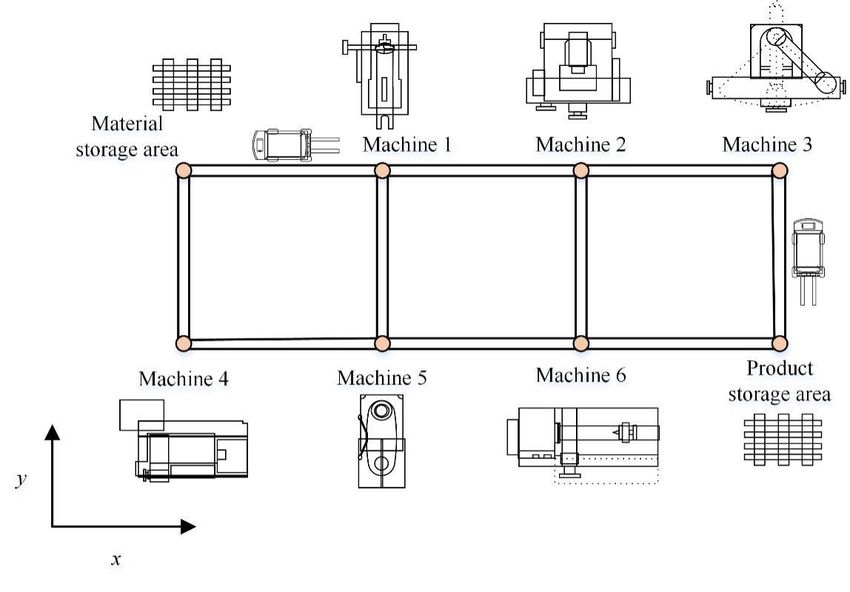
opportunities for future study are discussed in Section 5.

2. Problem description and formulation

 An FMC consists of M machines and V identical AGVs. A set of jobs j (j=1, 2, …, J) are to be
processed and transported through the FMC, and job j is composed of operations. Operation 
(k=1, 2, …, ) can be processed on a pre-determined set of machines ( ) with different process
time and process power.
 Figure 1 depicts an example of an FMC. Each node in the Figure represents an intersection where
the AGV can stop or turn, and the location of each node can be denoted to a coordinate. The node (0, 1)
is the location of the material storage area and the node (3, 0) is the location of the product storage area.
The remaining nodes house machines 1 to machine 6. Among the above nodes, those at which the two
storage areas are located allows all vehicles to stop at the same time, while the other nodes allow only
one vehicle to stop or pass at the same time. Some nodes are connected by lanes, and AGVs can only
travel on the lanes. All lanes can be entered from both ends, but any two AGVs cannot enter a lane from
its both ends at the same time. This is often the case due to the limited space in the workshop. The travel
speed of AGVs on the lanes can be considered as uniform, and the loading and unloading of jobs are
neglected. All the jobs and AGVs are located at material storage area at the beginning, and each job shall
be stored in the product storage area after completed.

 Figure 1. An example of an FMC.

 In the FMC, it is to decide the processing machine and processing sequence for each operation, the
AGV designated to each transfer and the transfer sequence, and to plan conflict-free transfer routes. The
goal of the BOGSP-FMC is to balance the two objectives of minimizing the total completion time and
total energy consumption of the manufacturing cell by making these decisions in a rational manner.

2.1. Assumptions

 To describe the problem more accurately, the following assumptions are made.
 (1) Each machine and AGV can process or handle only one job at a time, and each job can be
processed by only one machine or handled by one AGV at a time.
 (2) If two consecutive operations of a job are processed on the same machine, the job does not need
to be handled by an AGV between the two operations.
 (3) The AGVs travel on the lanes with uniform speed.
 (4) The setup times of the machines are not considered.
 (5) The loading and unloading time of the AGV is ignored or incorporated in the travel time.
 (6) Recharge of AGVs and equipment failure are not considered, and the AGVs and machines are
always available throughout the manufacturing process.

2.2. Mathematical model

 Based on the problem formulated, a mathematical model is proposed as an accurate depiction of the
BOGSP-FMC. The notations and explanations used in this model are listed in Table 1 and the
mathematical model is given as follows.

 Table 1. Notations and explanations.
 Notations Explanation
 j Job (j = 1, 2, …, J)
 Operation ( = 1, 2, … , , + 1) , and operation + 1 is dummy in
 k
 which the job is handled to the product storage area
 The kth operation of job j
 m Machine (m=1, 2, …, M, M +1), and M +1 denotes product storage area
 v AGV (v=1, 2, …, V)
 ( ) The set of machines which can choose
 The chosen processing machine of 
 
 The process time of on machine m, where ∈ ( )
 
 The process power of machine m
 ( ) The starting time of processing 
 ( ) The finishing time of processing 
 
 Power consumption when the AGV is traveling unloaded
 Power consumption when the AGV is traveling with load
 ( ) The time when is loaded
 ( ) The time when is unloaded
 nodes (s = 0, 1, …, S) in the network of an FMC, in which 1 denotes the
 Node where the material storage area locates, denotes the product storage
 area and ( ) denotes machine m
 The set of nodes which is connected to by lanes
 t Time step (t = 0, 1…, T)
 
 ( 11 , 22 ) is 1 if 22 processed immediately after 11 on machine m
 ( 11 , 22 )
 or 0 otherwise

 
 is 1 if is the first operation processed by machine m or 0 otherwise
 
 is 1 if is the last operation processed by machine m or 0 otherwise
 
 ( 11 , 22 ) is 1 if 22 processed immediately after 11 on AGV v or 0
 ( 11 , 22 )
 otherwise
 
 is 1 if is the first operation handled by AGV v or 0 otherwise
 
 is 1 if is the last operation handled by AGV v or 0 otherwise
 
 is 1 if AGV v locates at node s at time t, or 0 otherwise
 
 is determined by ( 11 , 22 ) and is 1 if is processed by machine
 
 m, or 0 otherwise
 
 is determined by ( 11 , 22 ) and is 1 if is handled by AGV v, or
 
 0 otherwise

 = ( 1 , 2 ) (1)
 +1
 1 = ( ) (2)
 
 2 = + (3)

 = ∑ ∑ ∑ 
 (4)
 ∈ ( )
 
 = ∑{ • ∑ [ ( 11 , 22 ) • ∑ 
 ∑ | +1
 − |] +
 1 ≠ 2 : 1

 
 ∑ ∑ = 1, ∀ (13)
 
 ′ 
 ∑ ( 11 , 11 ) + ∑ ∑ ( 11 , 22 ) + 1 1 = 1 1 , ∀ 1 , 1 , (14)
 1′ > 1 1 ≠ 2 2
 ′ 
 ∑ ( 11 , 11 ) + ∑ ∑ ( 22 , 11 ) + 1 1 = 1 1 , ∀ 1 , 1 , (15)
 1′ 1 ) (22)
 
 1 ( ) ≥ 0, ∀ (23)
 ( ) ≥ −1 ( ), ∀ , > 1 (24)
 ≥ ( ), ∀ , 
 ( ) (25)
 
 ( ) = → ( ) 
 ≥ (1 − ) ∙ ( −1) 
 ∙ , ∀ , > 1, , , (26)
 
 ( ) = 
 → ( ) ≥ (1 − ( −1) ) ∙ ∙ 
 , ∀ , , , , (27)
 
 ( ) ≥ ( ), ∀ , (28)

 ( ) = ( ) + ∑ 
 , ∀ , 
 (29)
 ∈ ( )

 ( 11 , 22 ), ( 11 , 22 ), , , , 
 
 , ∈ {0,1}, ∀ , , , , , (30)

 Equation (2) and Equation (3) are the two objectives of the optimization model. The first one is the
make-span and the other one is the total energy consumed, consisting of energy used for processing (as
calculated in Equation (4)) and that utilized for transportation (as in Equation (5)). Equation (6) -
Equation (30) are the constraints that the decision variables must obey. Equation (6) and Equation (7)
make sure that the first operation and the last one processed by each machine are unique. Equation (8)
– Equation (10) ensure each operation of each job is designated to only one machine. That one machine
can only process one operation of one job at the same time is guaranteed by Equation (11). Equation
(12) - Equation (16) are constraints related to AGVs which are like Equation (6) - Equation (10).
Equation (17) – Equation (21) are locational and conflict-free restrictions of AGVs. Equation (22)
ensures a job can only be loaded on an AGV after the immediate predecessor is unloaded. Equation (23)
and Equation (24) make sure a job can only be loaded on the AGV after the precedent operation is done.
Equation (25) guarantees the unloading time is latter than the loading time of each transportation task.
Equation (26) and Equation (27) ensure that loading and unloading can only be done at the correct node.
Equation (28) guarantees the process of each operation can only begin after the job is unloaded, and
Equation (29) makes sure the process is non-preemptive. Equation (30) declares that some of the

variables can only be zero or one.

3. Improved multi-objective salp swarm algorithm based on decomposition

 The BOGSP-FMC studied in this paper is an extension of the flexible job shop scheduling problem,
so it is NP-hard and most suitable to be solved by meta-heuristics. So, an improved multi-objective salp
swarm algorithm based on decomposition (IMOSSA/D) is proposed, which is based on the hybridization
of MOEA/D and an improved salp swarm algorithm (SSA). First, the initial population is generated
randomly. The crossover operator in MOEA/D is substituted by three crossover operators organized by
a competition mechanism. Also, three mutation operators based on stochastic distribution, namely
Brownian motion, Cauchy motion and Lévy flight are randomly chosen after the SSA to perform local
search of the individuals in the population. The framework of the proposed algorithm is shown in Figure
2.

 Figure 2. The framework of the IMOSSA/D.

 The proposed approach is presented in four parts in this section. First, a real number-based solution
representation is proposed and illustrated by a numerical example. Then, a conflict-free routing method

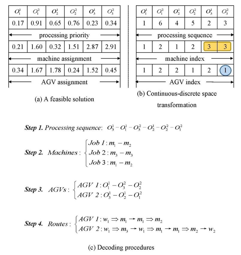
based on ACO is presented, in which a conflict avoidance mechanism is designed. Thereafter, a repair
mechanism is introduced to fix any infeasible solutions that arise during the evolution of the algorithm.
Finally, the composition of IMOSSA/D is described in detail, and the computational complexity of
IMOSSA/D is analyzed.

3.1. Solution representation

 Careful design of encoding and decoding methods is required when applying metaheuristics to solve
specific discrete optimization problems. A three-layer real-number-based solution representation is
proposed, each layer of which represents the processing order, machine assignment, and the assignment
of AGVs respectively.
 All the three layers of a solution is a vector of ∑ elements, each of which corresponds to one
operation of one job. The elements of the first layer are real numbers which belongs to [0,1], indicating
the priority of their operations. The smaller the number, the higher the priority. In the second layer are
real numbers belonging to [0, | ( )|], and a number which belongs to [0,1) represents that machine
1 is assigned, and so on. The third layer consists of real numbers between [0, ] for assigning AGVs.
 The decoding procedures are to interpreting the solution representation and to calculate the two
objectives. The details of them are listed as follows.
 Step 1. Obtain the processing order of each operation from the first layer of the solution.
 Step 2. Allocate machines to operations and record the processing sequence of machines.
 Step 3. Allocate AGVs to operations and record the transporting sequence of AGVs. When two
adjacent operations of the same job are processed on the same machine, the latter operation will not
require AGV handling.
 Step 4. Identify the starting, loading and unloading nodes of each AGV.
 Step 5. From t = 0, start the process and handling in FMCs and identify the state of jobs (operations
processed), machines (tasks performed) and AGVs (tasks performed and locations et al.) of each timestep.
These states can only and must be changed when the required constraints are met.
 To show the decoding process more clearly, an example is given for illustration. As shown in Figure
3, 3 jobs are involved, each of which contains 2 operations. The jobs are processed by 3 machines and
handled by 2 identical AGVs, and the 3 machines can process any operation of any job (for
simplification). Figure 3 (a) gives the representation of a feasible solution. Figure 3 (b) performs a
continuous-discrete-space transformation, converting the real numbers into processing priority and
indexes of machines/AGVs. Figure 3 (c) gives the decoding procedures based on step 1 to step 4. In the
handling route presented in step 4, ⇒ denotes a loaded route and → denotes an unloaded route. It is
worth noting that the AGV indexes in Figure 3 (b) highlighted by a circular box are two adjacent
operations of the same job which are processed on the same machine. So, the operation 32 does not
require handling.

Figure 3. An example of decoding procedures.

3.2. Conflict-free routing method

 By decoding steps 1-4, the starting node, end node and load of each AGV for each handling task are
obtained, meeting the prerequisites for routing. The proposed routing method is based on the ACO
(Dorigo et al. 1996), the main steps of which are as follows. At time step t, if the AGV is located at point
(x, y), it can change to five optional states ( +, −, +, − and stay) at moment + 1. Each one is
assigned a certain state transfer probability, and the action of each AGV between time step t and + 1
is determined randomly according to the above probabilities until it arrives at the end node. The ACA is
designed to gradually optimize the state transfer probability and thus to find a shorter path.
 To decide the action of each AGV between time step t to + 1, whether it is close to the end node is
the first concern, and then, possible route conflicts must be considered. Under certain circumstances, an
AGV choosing the best direction may force other AGVs to take a detour to avoid conflicts. The proposed
ACA copes with the above problem by introducing randomness and pheromone mechanism.
 
 Specifically, state transfer probability ( , , ) denotes the probability that an AGV chooses state
d at point (x, y) in the lth move. where s denotes the number of stages of the ACA and a is the index of

ants. It is calculated as follows.
 
 ( ,
 [ 
 ( , )] ∙ [ ( )] 
 , ) = (31)
 ∑ [ 
 ( , )] ∙ [ ( )] 
 
where ( ) is the heuristic function, obtained from Equation (32), and ( , ) denotes the
pheromone concentration of the AGV selecting state d at the point (x, y). When all ants have completed
 
the pathfinding, ( , , ) must be updated according to Equation (32), (33) and (34).

 > 1, ℎ 
 ( ) = { (32)
 1, otherwise
 
 ( , + 1) = (1 − ) ( , ) + ( , ) (33)
 ( , , )
 Δτ xy
 d
 (l , s) =∑[Δτ xy
 d
 (l , s, a)/T (l , s, a)] Δ ( , ) = ∑ Δ 
 (34)
 a ( , , )

 In Equation (34), the initial value of ( , , ) is 0, which will increase ( , , )
 each time ant a

selects that path (action). ( , , ) denotes the total time consumed by ant a in that handling task.
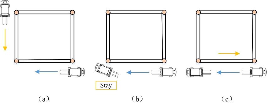
 A conflict elimination mechanism is designed for path conflicts of multiple AGVs. Three types of
conflicts may occur among AGVs as shown in Figure 4. When the current time step is t, the steps of path
planning at time + 1 are as follows.
 Step 1. Determine the priority order of path selection of each AGV.
 Step 2. Determine the action at time + 1 of the unacted AGV of the highest priority randomly
 
according to ( , , ), and any conflicts with acted AGVs must be avoided.
 Step 3. Check the state selection probability of each travel direction of the unacted AGVs. If there is
an AGV with state selection probability of 0 for each direction, withdraw the action of the AGV in step
2 and prohibit the AGV from selecting that action again. If there is unacted AGVs left, go back to step 2,
otherwise end path selection.

 Figure 4. Three types of routing conflicts.

3.3. Infeasible solution repair mechanism

 Infeasible solutions may be produced during the iterations of the IMOSSA/D, which can be repaired
to be feasible. There are two types of infeasibility that can be generated. First, the elements of a solution

may surpass the prescribed upper or the lower bound, which can be repaired by randomly regenerating
another real number in the predetermined range. Secondly, the processing sequence of the operations of
the same job may be violated. Infeasibility of this type can be repaired by rearrange the processing
priority of the same job in the first layer of the infeasible solution in ascending order. These repair
mechanisms can preserve the information contained in the infeasible solutions to the maximum extent
and transform them into feasible solutions.
 The repair mechanisms are illustrated with the example introduced in 3.1. An example of infeasible
solution before and after repair is shown in Figure 5 (a) and Figure 5 (b) respectively. First, the blue
ellipse identifies the first type of infeasibility and its repair. The infeasible element in the three layers of
the solution are out of bounds [0,1] , [0,3] and [0,2] , respectively, and the repair process is to
regenerate the values randomly within the respective range. Then, the yellow box identifies the second
type of infeasibility and its repair: the processing priority of the two operations of Job 2 violate the
constraint, thus they are rearranged in ascending order to repair.

 Figure 5. An example of the repair mechanism.

3.4. Population initialization

 The IMOSSA/D is designed based on MOEA/D, which, like other variants of MOEA/D, needs to
transform the multi-objective optimization problem into a set of scalar subproblems with a certain
decomposition method. The Chebyshev decomposition is employed, and thus the subproblems obtained
by the decomposition can be defined as follows.

 ( | , ∗ ) = { | ( ) − ∗ |} (35)
 1≤ ≤ 

where ∗ denotes the reference point, m is the number of objectives, is the weight vector assigned
to each subproblems.
 Based on this decomposition method, the initial population of the IMOSSA/D is generated by the
procedures as follows.
 Step 1. Randomly initialize a set of weight vectors 1 , 2 , . . . , , . . . , , where N is the population
size. Initialize the external archive = ∅.
 Step 2. For each weight vector , calculate the Euclidean distance between it and the rest of the

weight vectors. And find the T weight vectors with the closest distance corresponding to T neighborhood
solutions.
 Step 3. Randomly generate N initial solutions 1 , 2 , . . . , . . . , , each of which corresponds to
one subproblem. Calculate the m objectives of each solution.
 Step 4. Initialize the reference point ∗ , ∗ = 1≤ ≤ { ( )}, 1≤ ≤ . The objectives of each
subproblem, ( ), 1 ≤ ≤ , are obtained by solving Equation (35).

3.5. Competition mechanism of crossover operators

 The crossover operator in MOEA/D randomly selects two solutions and performs a simulated binary
crossover (SBX), and the child solutions will replace the parent solutions if they are better. This crossover
operator allows the solutions of subproblems to exchange information with each other during the
evolution and is the core operator of MOEA/D. It has been shown that the use of multiple operators is
better for maintaining the diversity of the population than the use of a single SBX (Wang et al. 2020),
avoiding the cliff decline of diversity in the late iterations. Inspired by this, this paper proposes the
competition mechanism of multiple crossover operators.
 First, uniform crossover (UX), two-point crossover (TPX) and SBX, which have superior
performance and large differences, are selected as alternative operators. For each crossover operator, one
crossover operator , = 1, 2, is chosen randomly according to the selection probability.
 / 
 ( ) = 
 (1 − ) + (36)
 ∑ / 
 
where is the contribution of in the last t iterations. The contribution is defined as the number of
times the parent solution is replaced by the children generated by the operator.

3.6. Improved salp swarm algorithm

 SSA is a swarm-intelligence-based meta-heuristic proposed by Mirjalili et al. (2017). The
metaheuristic, inspired by the behavior of salp swarms in nature, not only performs well in solving the
benchmark problems, but also has been applied by researchers to optimization problems such as electric
power dispatch (Kansal and Dhillon 2020), feature selection (Hegazy et al. 2020), wind power prediction
(Pan et al.) for practical applications.
 The salp swarm in nature spontaneously form "chains" to find food sources. SSA divides the entire
population into one leader and the followers. The leader is the individual leading the swarm at the front
of the chain, while the other individuals follow each other one by one. Like other swarm intelligence
algorithms, the position of a salp within the search space is determined by a n-dimensional vector. It is
also assumed that there is a food source F in the search space as the target of the swarm. The location of
the leader is updated according to Equation (36).
 + 1 (( − ) 2 + ) 3 ≥ 0
 1 = { (37)
 − 1 (( − ) 2 + ) 3 < 0
where, 1 is the coordinate of the position of the first salp (leader) in the j-th dimension. is the j-th
dimension of coordinate of the food source. and are the upper and the lower bound of the j-th
decision variable and 1 , 2 and 3 are random numbers.
 Equation (36) indicates that the leader salp update its position only according to the food source,
which is the best individual of the previous generation population. 1 is made adaptive with iterations
as in Equation (37) while 2 and 3 are uniform random numbers between [0,1].

4 2
 1 = 2 −( ) (38)

where l is the current number of iteration and L is the maximum one.
 The positions of the followers are updated as Equation (38).
 1
 = ( + −1 )， ≥ 2 (39)
 2
 SSA is modified in three ways as follows to adapt to the BOGSP-FMC with two objectives, decision
variables of high dimension and complex search space.

(1) Food source updating

 In the original single-objective SSA, the food source is the best optimal solution of the previous
generation population, which must be modified to solve a multi-objective problem. The best solutions
chosen from the historical populations are saved into the EA. Thus, the food source is a solution selected
from EA with roulette method.

(2) Updating the position of the followers

 The updating equation for the followers in original SSA enables full ability of exploration in the
earlier stage of the evolution. But the exploitation of the followers is rather less, which can make them
abandon some promising area in the search space, especially for a multi-objective one. In the same time,
the followers have no memory about their historical positions, which are underutilized. Hence Equation
(38) is modified as Equation (39).

 = + 4 ⋅ 1 ⋅ ( , − ) + 5 ⋅ 2 ⋅ ( −1 − )， ≥ 2 (40)

where 4 is the memory coefficient， 5 denotes the following coefficient， 1 and 2 are uniform
random numbers between [0,1], and , denotes the historical best position updated by Equation
(40).
 , ( ), ( ( + 1)) > ( , ( ))
 , ( + 1) = { (41)
 ( + 1), ℎ 

3.7. Stochastic-distribution-based operators

 Brownian motion, Cauchy motion and Lévy flight are three main stochastic-distribution-based
methods, all of which are now widely used in the field of intelligent optimization. Among these three
operators, Brownian motion has a smaller step size and stronger local search ability; Cauchy motion has
a larger step size, which can improve the global search ability of the algorithm; and Lévy flight has small
steps mixed with occasional large steps, which can effectively help avoid premature of the algorithm. A
combination of the three operators is added to the IMOSSA/D, which can take advantage of all three at
the same time. The mathematical expression of Brownian motion is as follows.
 , = + ⊕ (42)
 , 
where is the initial solution and 
 is the child one, is the step size coefficient, ⊕ denotes
multiplying by elements, and B obey the standard normal distribution.
 The expression of Cauchy motion is as follows.

 , = + ⊕ (43)
where C obey the Cauchy distribution, the distribution function of which is Equation (44).
 = × ( ( − 1/2)) (44)
where = 1 is the proportional coefficient and y obeys the standard uniform distribution.
 The expression of Lévy flight is presented in Equation (45).
 , = + ⊕ ( ) (45)
where ( ) obeys Lévy distribution, which can be generated as in Equation (46) when 0.3 ≤ ≤
1.99.
 
 ( ) = 0.05 × (46)
 | |1/ 
 where ∼ (0, 2 ) and ∼ (0, 2 ) , and these coefficients are calculated as
follows.
 1/ 
 (1 + ) 
 = [ 2
 −1 ] = 1 = 1.5 (47)
 1+ 
 ( ) 2 2
 2

3.8. External archive maintenance with quality indicator

 An EA is introduced to document best solutions generated during the iterations of the metaheuristic,
which may not be preserved otherwise. An EA is usually updated with non-dominated sorting and
crowding degree indicator. Binary-indicators are promising to compare two solution sets, with lower
computational cost and better reflection of dominance relationships. The ε-quality indicator proposed by
Luo et al. (2018) is utilized to update EA.
 Let population P be a sample in the decision space , and the fitness ( ) of an individual ∈ 
is defined in Equation (48), (49) and (50).
 ( ) = ∑ ({ }, { }) (48)
 ∈ \ 

 ({ }, { })=- ( − ({ }, { })/( × )) (49)

 ( , ) = {∀ ∈ ∃ ∈ : ( ) − ≤ ( )} ∈ {1,2, . . . , } (50)
 
where = 
 , ∈ 
 | ( , )|, and = 0.01 is the proportional coefficient. ( ) measures the “quality”

lost if x is removed from P, which is thus called quality indicator.
 The EA is updated by steps as follows.
 Step 1. Combine EA and the current generation P to get = ∪ , Retain only the non-dominant
solutions in S by non-dominant sorting.
 Step 2. If number of the solutions in S (| |) is no more than , Make = and the updating
is finished, otherwise go to Step 3.
 Step 3. Eliminate one solution with the smallest ( ) at a time, until | | = .

3.9. Computational complexity analysis

 Let the population size be N, the number of objectives be m, and the number of the decision variables
be D, then the computational complexity of each ingredient of the IMOSSA/D is listed in Table 2. As
can be seen in the table, the computational complexity of the proposed approach is ( 2 + ).

Table 2. Computational complexity analysis.
 Ingredient of the IMOSSA/D Computational complexity
 Population initialization ( )
 Competition mechanism of
 ( )
 crossover operators
 Improved SSA ( )
 Stochastic-distribution-based
 ( )
 operators
 EA maintenance ( 2 )
 Total ( 2 + )

4. Computational experiments

 To evaluate the performance of the IMOSSA/D proposed in this paper, it is implemented with Python
to solve a set of test problem instances with different features. First, the way these test problems are
generated is described in detail. Then, a set of performance indicators are introduced to evaluate the
multi-objective algorithm. Next, evaluated with the indicators, the proposed algorithm is compared with
two state-of-the-art intelligent algorithms on FJSSP, MOGWO (Luo et al. 2019) and PLMEAPS (Zhou
and Liao 2020). Thereafter, the effects of the major ingredients of the IMOSSA/D are verified
experimentally.

4.1. Problem instances and parameters

 The problem instances are generated randomly, since there are no benchmark problems in the
literature. The locations of the machines and storage areas are random. The number of operations of each
job in one instance is designated from discrete uniform distribution [1, 5]. The process time of each
operation is generated from [10, 50], and the process power of each machine from [10, 20]. The
transfer power of any AGV is 8 if empty or 15 otherwise. Each problem instance can be represented by
a combination of codes J, M and V representing the number of jobs, the number of machines and the
number of AGVs, respectively. For instance, J20M5V2 represents an instance involving 20 jobs, 5
machines and 2 AGVs. These instances are divided into three groups including small ( ≤ 100), medium
(100 ≤ ≤ 200) and large ones ( > 200) by the number of jobs involved.
 The three involved algorithms are executed 15 times on each problem instances with different random
seeds, on a PC with Intel Core i5 2.9GHz CPU and 16 GB RAM.

4.2. Performance indictors

 A set of unary indicators are introduced to evaluate the involved algorithms including the degree of
pareto optimality (DPO), generational distance (GD), diversity (Δ) and hyper volume (HV) (Zhou and
Zhu 2021b).

(1) DPO measures the number of pareto solutions obtained by one algorithm, defined as follows.

 | ∩ ∗ |
 = (51)
 | ∗ |
where is the pareto front obtained by the involved algorithm while ∗ denotes the true pareto
front.

(2) GD indicates the convergence degree of solution sets, denoted as follows.

 √∑| | 2
 =1 (52)
 =
 | |
where is the Euclidean distance between the i-th solution in PF and ∗ .

(3) Δ is the measure of diversity and evenness, and a smaller Δ indicates a solution set with more

 desirable distribution, defined as follows.

 −
 | |
 ∑ 
 =1 + ∑ =1 | − |
 = − (53)
 ∑ 
 =1 + | | 
 −
where is the Euclidean distance between the i-th solution in PF and the others, denotes the mean
value of , is the Euclidean distance between the extreme solution of the j-th dimension of PF and
 ∗ , and m denotes the number of objectives.

(4) HV is the volume of the hyper-polyhedron enclosed by the non-dominated solutions and the

reference point in the search space, measuring the degree of dispersion and convergence of the solution

sets, defined in Equation (54).

 | |
 = (∪ =1 ) (54)

where represents the Lebrun measure and is the volume of the hypercube enclosed by the i-th
solution and the reference point.

4.3. Parameter tuning

 The parameters of the algorithms are tuned with Taguchi method(Zhou and He 2021), which is a
widely used method for deciding the values of multiple parameters. For problem of different size,
different values are chosen by the Taguchi method. The parameter settings for the approaches involved
in the experiment are shown in Table 3.
 Table 3. Parameter settings of the three algorithms.

Parameter setting
 Algorithm Parameter
 Small Medium Large

 Population size 100 100 100

 Iteration 100 200 300

 Neighbor size 10 10 10
 IMOSSA/D
 Memory coefficient 0.8 0.8 0.8

 Following coefficient 0.2 0.2 0.2

 Step size 0.5 0.5 0.5

 Population size 100 100 100

 Iteration 100 200 300

 MOGWO Crossover rate 0.8 0.8 0.8

 Variation rate 0.1 0.1 0.1

 μ 0.03 0.03 0.03

 Population size 100 100 100

 Iteration 100 200 300

 EA size 100 100 100
 PLMEAPS
 Neighbor size 10 10 10

 Inertia weight 0.9 0.9 0.9

 Learning coefficient 2 2 2

4.4. Experimentation and analysis of results

 Ninety problem instances are designed according to 4.1 to evaluate the performance of the proposed
method and the two benchmark methods, where 5 machines and 1 to 3 vehicles are involved. The
performance of the three algorithms on problem instances of different sizes is analyzed by dividing all
problem instances into three groups according to their size, i.e., the number of jobs involved. The
instances involving 10 to 100 jobs are small instances, those involving 110 to 200 jobs are medium sized
ones and those containing 210 to 300 jobs are divided into large-scale group. The performance of the
three algorithms on problems of 3 different scale is measured by the four indicators defined in 4.2 and is
shown in Figure 6-8. Then, several conclusions can be drawn as follows.

(1) According to the DPO indicator, the IMOSSA/D can find more pareto solutions than the other two
 methods in 24 out of 30 small-scale problems, 29 out of 30 medium-sized problems and 30 out of
 30 large problems. Thus, the quantitative advantage of the IMOSSA/D exists at all problem sizes
 and expands as the problem size increases.

(2) Based on GD indicator, which measures the convergence rate of a solution set, it can be concluded
 that the solution sets obtained using the IMOSSA/D is superior to the benchmark methods at 25
 out of 30 small instances, 29 out of 30 medium sizes instances and 26 out of 30 large instances.

(3) As for Δ indicator, the IMOSSA/D takes no advantage in diversity and evenness in the three
 methods. The proposed approach is better than the benchmarks in 10 small instances, 7 medium
 instances and 5 large instances.

 (4) In view of the HV indicator, the IMOSSA/D is almost always better than the others
 except for one medium instance, demonstrating its high overall performance.

 IMOSSA/D PLMEAPS MOGWO IMOSSA/D PLMEAPS MOGWO
 1 0.1
 0.8 0.08
 0.6 0.06
 0.4 0.04
 0.2 0.02
 0 0
 0 5 10 15 20 25 30 0 5 10 15 20 25 30
 
 IMOSSA/D PLMEAPS MOGWO IMOSSA/D PLMEAPS MOGWO
 1 1

 0.8 0.8

 0.6 0.6

 0.4 0.4

 0.2 0.2

 0 0
 0 5 10 15 20 25 30 0 5 10 15 20 25 30
 
 Figure 6. Experimental results of 30 small sized problem instances.

IMOSSA/D PLMEAPS MOGWO IMOSSA/D PLMEAPS MOGWO
 1 0.1

0.8 0.08
0.6 0.06
0.4 0.04
0.2 0.02
 0 0
 0 5 10 15 20 25 30 0 5 10 15 20 25 30
 
 IMOSSA/D PLMEAPS MOGWO IMOSSA/D PLMEAPS MOGWO
 1 1

0.8 0.8

0.6 0.6

0.4 0.4

0.2 0.2

 0 0
 0 5 10 15 20 25 30 0 5 10 15 20 25 30
 
 Figure 7. Experimental results of 30 medium sized problem instances.

IMOSSA/D PLMEAPS MOGWO IMOSSA/D PLMEAPS MOGWO
 1 0.1

 0.8 0.08
 0.6 0.06
 0.4 0.04
 0.2 0.02
 0 0
 0 5 10 15 20 25 30 0 5 10 15 20 25 30
 
 IMOSSA/D PLMEAPS MOGWO IMOSSA/D PLMEAPS MOGWO
 1 1

 0.8 0.8

 0.6 0.6

 0.4 0.4

 0.2 0.2

 0 0
 0 5 10 15 20 25 30 0 5 10 15 20 25 30
 
 Figure 8. Experimental results of 30 large sized problem instances.

 Considering the random nature of the meta-heuristics and the generated problem instances, paired T-
tests (Table 4) are performed to determine whether there are significant differences between the
performance of the proposed algorithm and the benchmark methods with a confidence level of 95% (all
the samples have passed the normality tests and the equivariance tests). The results shown in Table 4
demonstrate that the IMOSSA/D is significantly superior to the benchmarks at DPO, GD and HV
indicators and there is no significant difference between the three methods at Δ indicator.

 Table 4. Paired T-tests on the performance of the IMOSSA/D versus the benchmark methods.
 Metric Problem size Benchmark T value P value
 MOGWO 11.43 0.00
 Small
 PLMEAPS 7.04 0.00
 MOGWO 11.52 0.00
 Medium
 PLMEAPS 18.11 0.00
 MOGWO 12.28 0.00
 Large
 PLMEAPS 17.59 0.00
 MOGWO -5.31 0.00
 Small
 PLMEAPS -7.63 0.00
 MOGWO -6.96 0.00
 Medium
 PLMEAPS -10.27 0.00

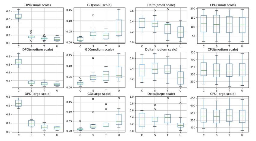
MOGWO -6.09 0.00
 Large
 PLMEAPS -6.26 0.00
 MOGWO -0.06 0.95
 Small
 PLMEAPS 0.50 0.62
 MOGWO -1.03 0.31
 Medium
 PLMEAPS -0.50 0.62
 MOGWO -2.21 0.53
 Large
 PLMEAPS -2.15 0.44
 MOGWO 11.25 0.00
 Small
 PLMEAPS 9.76 0.00
 MOGWO 9.98 0.00
 Medium
 PLMEAPS 14.76 0.00
 MOGWO 10.95 0.00
 Large
 PLMEAPS 18.54 0.00

(4) 4.5. Effect of the competition mechanism of crossover operators

 The competition mechanism of crossover operators chooses one from the three operators at a time
based on their contribution. So, the computational cost of it almost equals to just using one crossover
operator. However, the superiority of the mechanism should be justified in comparison with those which
utilize only one crossover. MOEA/D with this mechanism is denoted as C, and that with SBX, TPX or
UX as S, T and U. The experimental results are shown in box-plots as in Figure 6.

 Figure 9. Performance of C, S, T and U.

 The and values of C are better than the other three methods with acceptable degree of
variation. Algorithm U has the smallest value, while that of the other three algorithms do not differ
much. The mean value and variation of the of all methods are almost the same, consistent with the

previous analysis.

4.6. Effect of the improved salp swarm algorithm

 The improved salp swarm algorithm is denoted as M, while MOEA/D hybridized with SSA is S and
MOEA/D is D. These three algorithms run independently fifteen times for problem instances of different
scale. The experimental results are listed in Table 11, where and denote normalized mean
maximum completion time and mean total energy consumption of the pareto front. Indicator denotes
the average number of iterations (rounded up) where of M starts to be less than those of the other
two algorithms. Flag indicates the dominance state of M, and if and of M are both smaller
than those of S and D, then Flag = +1; if they are both larger, then Flag = -1; otherwise Flag = 0.
 In Table 8, it can be seen that and of M are the smallest most of the time. In view of
indicator Flag, it takes the value of +1 for 21 times out of the 30 instances. of M takes the largest
value for 28 times, and usually maintains this advantage from earlier iterations, as seen by indicator .

 Table 5. Performance of D, M and S.
 M S D
 Instance Flag
 
J10M5V1 4.59E+02 7.11E+03 0.662 4.78E+02 7.45E+03 0.314 5.36E+02 8.24E+03 0.108 37 +1
J20M5V1 1.42E+03 1.88E+04 0.715 1.59E+03 2.02E+04 0.556 1.65E+03 2.27E+04 0.535 84 +1
J30M5V1 4.59E+02 2.99E+04 0.687 1.81E+03 2.99E+04 0.389 1.87E+03 3.15E+04 0.455 79 0
J40M5V1 3.81E+03 5.30E+04 0.773 3.80E+03 5.27E+04 0.749 3.86E+03 5.50E+04 0.635 81 -1
J50M5V1 3.52E+03 4.81E+04 0.816 3.64E+03 5.18E+04 0.389 3.95E+03 5.36E+04 0.370 57 +1
J60M5V1 4.66E+03 3.84E+04 0.699 4.54E+03 3.99E+04 0.423 5.18E+03 4.22E+04 0.329 42 0
J70M5V1 6.19E+03 9.16E+04 0.724 6.22E+03 9.33E+04 0.482 6.85E+03 9.91E+04 0.316 53 +1
J80M5V1 7.54E+03 9.73E+04 0.844 7.69E+03 9.86E+04 0.258 8.29E+03 1.08E+05 0.250 82 +1
J90M5V1 1.73E+04 2.01E+04 0.634 1.77E+04 2.23E+04 0.324 2.03E+04 2.32E+04 0.279 76 +1
J100M5V1 6.35E+03 8.20E+04 0.714 6.58E+03 8.77E+04 0.479 6.89E+03 8.87E+04 0.385 65 +1
J110M5V1 1.73E+04 2.38E+05 0.792 1.79E+04 2.44E+05 0.669 1.84E+04 2.44E+05 0.444 135 +1
J120M5V1 1.35E+04 1.83E+05 0.668 1.42E+04 1.88E+05 0.541 1.41E+04 1.90E+05 0.499 147 +1
J130M5V1 2.39E+04 3.65E+05 0.604 2.39E+05 3.72E+05 0.439 2.40E+04 3.52E+05 0.580 192 0
J140M5V1 1.91E+04 2.86E+05 0.421 1.87E+05 2.81E+05 0.588 1.92E+04 2.92E+05 0.380 - -1
J150M5V1 1.61E+04 2.36E+05 0.849 1.63E+05 2.38E+05 0.766 1.81E+04 2.57E+05 0.532 81 +1
J160M5V2 1.55E+04 2.44E+05 0.810 1.57E+05 2.45E+05 0.509 1.67E+04 2.51E+05 0.268 152 +1
J170M5V2 2.58E+04 3.63E+05 0.661 2.65E+05 3.66E+05 0.422 2.37E+04 3.56E+05 0.405 78 +1
J180M5V2 2.29E+04 3.31E+05 0.66 2.29E+05 3.38E+05 0.401 2.37E+04 3.56E+05 0.443 93 0
J190M5V2 2.05E+04 2.94E+05 0.795 2.13E+05 2.92E+05 0.549 2.18E+04 3.13E+05 0.307 171 0
J200M5V2 1.35E+04 2.23E+05 0.687 1.50E+05 2.38E+05 0.560 1.54E+04 2.59E+05 0.476 74 +1
J210M5V2 2.64E+04 3.68E+05 0.807 2.70E+05 3.76E+05 0.685 2.83E+04 3.89E+05 0.340 146 +1

J220M5V2 3.09E+04 4.73E+05 0.825 3.19E+05 4.83E+05 0.448 3.41E+04 5.19E+05 0.413 153 +1
J230M5V2 3.40E+04 4.88E+05 0.638 3.46E+05 4.95E+05 0.504 3.55E+04 5.20E+05 0.396 239 +1
J240M5V2 3.70E+04 6.17E+05 0.601 3.71E+05 6.12E+05 0.267 3.92E+04 6.49E+05 0.263 186 +1
J250M5V2 3.71E+04 4.88E+05 0.788 3.74E+05 4.93E+05 0.407 3.98E+04 5.26E+05 0.394 231 +1
J260M5V3 3.03E+04 4.56E+05 0.627 3.10E+05 4.60E+05 0.591 3.98E+04 5.26E+05 0.422 134 +1
J270M5V3 3.20E+04 4.19E+05 0.480 3.18E+05 4.13E+05 0.729 3.27E+04 4.26E+05 0.348 - -1
J280M5V3 3.20E+04 5.19E+05 0.755 3.35E+05 5.38E+05 0.496 3.38E+04 5.48E+05 0.423 249 +1
J290M5V3 4.21E+04 6.16E+05 0.797 4.19E+05 6.20E+05 0.657 4.28E+04 6.31E+05 0.456 177 0
J300M5V3 3.69E+04 5.37E+05 0.653 3.82E+05 5.56E+05 0.469 3.91E+04 5.68E+05 0.370 196 +1

4.7. Effect of the stochastic-distribution-based operators

 The justification of stochastic-distribution-based operators is performed in the same way as that of
the crossover operators. MOEA/D incorporated with all the three operators is denoted as LS, and those
with Brownian motion, Cauchy motion and Lévy flight are BM, CM and LF respectively. LS, BM, CM,
LF and D are run independently fifteen times for the problem instances and the results is shown in Figure
7.
 LS notably outperforms the other four algorithms in , and is also the best in for most of
the instances. However, LS has shown little advantage in over the other methods.

0.8
0.7 DPO
 LS BM CM LF D
0.6
0.5
0.4
0.3
0.2
0.1
 0

 GD
 LS BM CM LF D
 0.16
 0.14
 0.12
 0.1
 0.08
 0.06
 0.04
 0.02
 0

 Delta
 LS BM CM LF D
 0.9
 0.8
 0.7
 0.6
 0.5
 0.4
 0.3
 0.2
 0.1
 0

 Figure 10. Performance of RW, BM, CM, LF and D.

4.8. Managerial applications

 To bridge some gaps between the proposed approach and its real-world implementation, this section

is to put some insights in its managerial applications.
 The bi-objective approach pursues the tradeoff between two objectives and may yield multiple non-
dominant solutions. Then, it is for the decision makers to choose from the solutions. Different decision
makers may have different opinions on the importance of the two objectives, namely the make span and
the energy cost. Thus, a preference vector = ( 1 , 1 − 1 ), is used to describe the relative attention
given by decision makers to the two objective functions.
 The decision maker can take the value of 1 based on the relative importance of 1 and 2 . The
importance of 1 is positively correlated with the value of 1 . In this paper, the value of 1 is equally
divided into 5 intervals, namely [0, 0.2), [0.2,0.4), [0.4, 0.6), [0.6, 0.8), [0.8, 1], each of which
corresponds to an applicational scenario. As an illustrative example, a medium-scale problem instance
J150M5V2 is solved and the results is presented in Figure 11.

 Scenario 1 Scenario 2 Scenario 3 Scenario 4 Scenario 5
 225000
 220000
 Total energy consumption

 215000
 210000
 205000
 200000
 195000
 190000
 14500 15000 15500 16000 16500 17000
 Make span

 Figure 11. Solutions of J150M5V2 in different applicational scenarios

 As shown in the figure, the pareto solution set is divided into 5 groups according to different intervals
of preference vector and the number of alternatives left for decision makers is narrowed down.
 In sight of the managerial applications of the addressed problem in this section, we believe that this
study can provide the managers with an approach to create greener flexible manufacturing cells with
guaranteed productivity, making their enterprise more competitive and sustainable.

5. Conclusions and future research

 Inspired by the opportunity in introducing energy-efficient criterion and conflict-free routing for
AGVs in FMCs, this paper models a bi-objective green scheduling problem for flexible manufacturing
cells. A realistic consideration of AGV routing can bridge some gaps between research and engineering
practice. At the same time, energy costs incurred during processing and transportation, which are
complexly interlinked, is calculated in a more simplified way. To solve this problem, we designed an
approach based on MOEA/D. The approach absorbs three strategies to adapt the MOEA/D to the problem.
First, the competition mechanism of crossover operators substitutes the SBX in MOEA/D to enhance its

search ability. Then, an improved salp swarm algorithm and three stochastic-distribution-based operators
are also incorporated. At last, an external archive update method with quality indicator is introduced.
Computational experiments are performed to evaluate the proposed algorithm on the studied problem,
and it outperforms MOGWO and PLMEAPS. The three components of the IMOSSA/D are also validated
experimentally.
 Future study may involve other greening practice such as shutdown reboot policies and processing
speed tuning. In addition, more practical consideration, such as battery depletion of AGVs and machine
downtime, can be introduced. As for the approach, the proposed meta-heuristic still has some weaknesses
in terms of solution diversity. Exact methods are also needed for smaller version of the studied problem.

Statements and Declarations

Funding

The authors declare that no funds, grants, or other support were received during the preparation of
this manuscript.

Competing Interests
The authors have no relevant financial or non-financial interests to disclose.

Ethical approval
This article does not contain any studies with human participants or animals performed by any of
the authors.

Author Contributions
All authors contributed to the study conception and design.
Binghai Zhou:
Proposed the research goals and aims. Verified the overall results, experiments and
other outputs. Provided the computing resources and analysis tools. Conducted the
statistical analysis. Reviewed the initial draft and revised the manuscript. In charge of
acquisition of the financial support for the project leading to this publication.
Jihua Zhang:
Developed and designed the mathematical model and methodology. Performed the
software development and experiments. Conducted the statistical analysis. Wrote the
initial draft and revised the manuscript.
All authors read and approved the final manuscript.

Data Availability
The datasets generated during and/or analysed during the current study are not
publicly available due to that the data also forms part of an ongoing study, but are
available from the corresponding author on reasonable request.

References

Balakrishnan K, Dhanalakshmi R and Khaire U M (2022) A novel control factor and brownian motion-
 based improved harris hawks optimization for feature selection. J. Ambient Intell. Humaniz.
 Comput.:23. https://doi.org/10.1007/s12652-021-03621-y
Barshandeh S, Dana R and Eskandarian P (2022) A learning automata-based hybrid mpa and js algorithm
 for numerical optimization problems and its application on data clustering. Knowledge-Based Syst.
 236:42. https://doi.org/10.1016/j.knosys.2021.107682
Bechtsis D, Tsolakis N, Vlachos D and Iakovou E (2017) Sustainable supply chain management in the
 digitalisation era: The impact of automated guided vehicles. Journal of Cleaner Production
 142:3970-3984. https://doi.org/10.1016/j.jclepro.2016.10.057
Chou Y L, Yang J M and Wu C H (2020) An energy-aware scheduling algorithm under maximum power
 consumption constraints. J. Manuf. Syst. 57:182-197. https://doi.org/10.1016/j.jmsy.2020.09.004
Chutima P and Arayikanon K (2020) Many-objective low-cost airline cockpit crew rostering optimisation.
 Computers & Industrial Engineering 150:12. https://doi.org/10.1016/j.cie.2020.106844
Dagal I, Akin B and Akboy E (2022) Improved salp swarm algorithm based on particle swarm
 optimization for maximum power point tracking of optimal photovoltaic systems. Int. J. Energy Res.
 46 (7):8742-8759. https://doi.org/10.1002/er.7753
Deb K, Pratap A, Agarwal S and Meyarivan T (2002) A fast and elitist multiobjective genetic algorithm:
 Nsga-ii. IEEE Transactions on Evolutionary Computation 6 (2):182-197.
Deliktas D, Ozcan E, Ustun O and Torkul O (2021) Evolutionary algorithms for multi-objective flexible
 job shop cell scheduling. Appl. Soft. Comput. 113:18. https://doi.org/10.1016/j.asoc.2021.107890
Diaz J L and Ocampo-Martinez C (2019) Energy efficiency in discrete-manufacturing systems: Insights,
 trends, and control strategies. J. Manuf. Syst. 52:131-145.
 https://doi.org/10.1016/j.jmsy.2019.05.002
Dong H, Xu Y L, Li X P, Yang Z L and Zou C H (2021) An improved antlion optimizer with dynamic
 random walk and dynamic opposite learning. Knowledge-Based Syst. 216
 https://doi.org/10.1016/j.knosys.2021.106752
Dorigo M, Maniezzo V and Colorni A (1996) Ant system: Optimization by a colony of cooperating agents.
 IEEE Trans. Syst. Man Cybern. Part B-Cybern. 26 (1):29-41.
 https://doi.org/10.1109/3477.484436
Feng Y X, Hong Z X, Li Z W, Zheng H and Tan J R (2020) Integrated intelligent green scheduling of
 sustainable flexible workshop with edge computing considering uncertain machine state. Journal of
 Cleaner Production 246:18. https://doi.org/10.1016/j.jclepro.2019.119070
Fontes D and Homayouni S M (2019) Joint production and transportation scheduling in flexible
 manufacturing systems. Journal of Global Optimization 74 (4):879-908.
 https://doi.org/10.1007/s10898-018-0681-7
Gao K Z, Cao Z G, Zhang L, Chen Z H, Han Y Y and Pan Q K (2019) A review on swarm intelligence
 and evolutionary algorithms for solving flexible job shop scheduling problems. Ieee-Caa Journal of
 Automatica Sinica 6 (4):904-916. https://doi.org/10.1109/jas.2019.1911540
Gao K Z, Huang Y, Sadollah A and Wang L (2020) A review of energy-efficient scheduling in intelligent
 production systems. Complex Intell. Syst. 6 (2):237-249. https://doi.org/10.1007/s40747-019-
 00122-6
Gupta S and Deep K (2019) A novel random walk grey wolf optimizer. Swarm Evol. Comput. 44:101-
 112. https://doi.org/10.1016/j.swevo.2018.01.001
He L J, Chiong R, Li W F, Budhi G S and Zhang Y (2022) A multiobjective evolutionary algorithm for