An Industrial-Strength Audio Search Algorithm - Columbia EE
←
→
Page content transcription
If your browser does not render page correctly, please read the page content below
An Industrial-Strength Audio Search Algorithm
Avery Li-Chun Wang
avery@shazamteam.com
Shazam Entertainment, Ltd.
USA:                                                                United Kingdom:
2925 Ross Road                                                      375 Kensington High Street
Palo Alto, CA 94303                                                 4th Floor Block F
                                                                    London W14 8Q

We have developed and commercially deployed a flexible audio search engine. The algorithm is noise and distortion resistant,
computationally efficient, and massively scalable, capable of quickly identifying a short segment of music captured through a
cellphone microphone in the presence of foreground voices and other dominant noise, and through voice codec compression, out
of a database of over a million tracks. The algorithm uses a combinatorially hashed time-frequency constellation analysis of the
audio, yielding unusual properties such as transparency, in which multiple tracks mixed together may each be identified.
Furthermore, for applications such as radio monitoring, search times on the order of a few milliseconds per query are attained,
even on a massive music database.

                                                                    30-second clip of the song to a friend. Other services, such
                                                                    as purchasing an MP3 download may become available
1 Introduction                                                      soon.
Shazam Entertainment, Ltd. was started in 2000 with the
idea of providing a service that could connect people to            A variety of similar consumer services has sprung up
music by recognizing music in the environment by using              recently. Musiwave has deployed a similar mobile-phone
their mobile phones to recognize the music directly. The            music identification service on the Spanish mobile carrier
algorithm had to be able to recognize a short audio sample          Amena using Philips’ robust hashing algorithm [2-4].
of music that had been broadcast, mixed with heavy                  Using the algorithm from Relatable, Neuros has included a
ambient noise, subject to reverb and other processing,              sampling feature on their MP3 player which allows a user
captured by a little cellphone microphone, subjected to             to collect a 30-second sample from the built-in radio, then
voice codec compression, and network dropouts, all before           later plug into an online server to identify the music [5,6].
arriving at our servers. The algorithm also had to perform          Audible Magic uses the Muscle Fish algorithm to offer the
the recognition quickly over a large database of music with         Clango service for identifying audio streaming from an
nearly 2M tracks, and furthermore have a low number of              internet radio station [7-9].
false positives while having a high recognition rate.
                                                                    The Shazam algorithm can be used in many applications
This was a hard problem, and at the time there were no              besides just music recognition over a mobile phone. Due to
algorithms known to us that could satisfy all these                 the ability to dig deep into noise we can identify music
constraints. We eventually developed our own technique              hidden behind a loud voiceover, such as in a radio advert.
that met all the operational constraints [1].                       On the other hand, the algorithm is also very fast and can
                                                                    be used for copyright monitoring at a search speed of over
We have deployed the algorithm to scale in our commercial           1000 times realtime, thus enabling a modest server to
music recognition service, with over 1.8M tracks in the             monitor significantly many media streams. The algorithm
database. The service is currently live in Germany,                 is also suitable for content-based cueing and indexing for
Finland, and the UK, with over a half million users, and            library and archival uses.
will soon be available in additional countries in Europe,
Asia, and the USA. The user experience is as follows: A
user hears music playing in the environment. She calls up           2 Basic principle of operation
our service using her mobile phone and samples up to 15             Each audio file is “fingerprinted,” a process in which
seconds of audio. An identification is performed on the             reproducible hash tokens are extracted. Both “database”
sample at our server, then the track title and artist are sent      and “sample” audio files are subjected to the same analysis.
back to the user via SMS text messaging. The information            The fingerprints from the unknown sample are matched
is also made available on a web site, where the user may            against a large set of fingerprints derived from the music
register and log in with her mobile phone number and                database.     The candidate matches are subsequently
password. At the web site, or on a smart phone, the user            evaluated for correctness of match.          Some guiding
may view her tagged track list and buy the CD. The user             principles for the attributes to use as fingerprints are that
may also download the ringtone corresponding to the                 they should be temporally localized, translation-invariant,
tagged track, if it is available. The user may also send a          robust, and sufficiently entropic. The temporal locality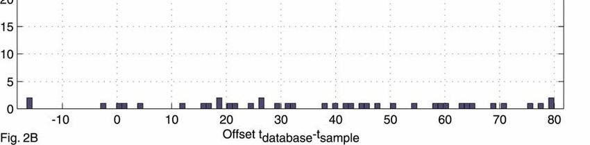
guideline suggests that each fingerprint hash is calculated
using audio samples near a corresponding point in time, so
that distant events do not affect the hash. The translation-
                                                               2.1    Robust Constellations
invariant aspect means that fingerprint hashes derived from    In order to address the problem of robust identification in
corresponding matching content are reproducible                the presence of highly significant noise and distortion, we
independent of position within an audio file, as long as the   experimented with a variety of candidate features that could
temporal locality containing the data from which the hash      survive GSM encoding in the presence of noise. We settled
is computed is contained within the file. This makes sense,    on spectrogram peaks, due to their robustness in the
as an unknown sample could come from any portion of the        presence of noise and approximate linear superposability
original audio track. Robustness means that hashes             [1]. A time-frequency point is a candidate peak if it has a
generated from the original clean database track should be     higher energy content than all its neighbors in a region
reproducible from a degraded copy of the audio.                centered around the point. Candidate peaks are chosen
Furthermore, the fingerprint tokens should have sufficiently   according to a density criterion in order to assure that the
high entropy in order to minimize the probability of false     time-frequency strip for the audio file has reasonably
token matches at non-corresponding locations between the       uniform coverage. The peaks in each time-frequency
unknown sample and tracks within the database.                 locality are also chosen according amplitude, with the
Insufficient entropy leads to excessive and spurious           justification that the highest amplitude peaks are most
matches at non-corresponding locations, requiring more         likely to survive the distortions listed above.
processing power to cull the results, and too much entropy
usually leads to fragility and non-reproducibility of          Thus, a complicated spectrogram, as illustrated in Figure
fingerprint tokens in the presence of noise and distortion.    1A may be reduced to a sparse set of coordinates, as
                                                               illustrated in Figure 1B. Notice that at this point the
There are 3 main components, presented in the next             amplitude component has been eliminated. This reduction
sections.                                                      has the advantage of being fairly insensitive to EQ, as
generally a peak in the spectrum is still a peak with the Yang also considered the use of spectrogram peaks, but
same coordinates in a filtered spectrum (assuming that the employed them in a different way [10].
derivative of the filter transfer function is reasonably
small—peaks in the vicinity of a sharp transition in the
transfer function are slightly frequency-shifted). We term
2.2 Fast Combinatorial Hashing
the sparse coordinate lists “constellation maps” since the Finding the correct registration offset directly from
coordinate scatter plots often resemble a star field. constellation maps can be rather slow, due to raw
constellation points having low entropy. For example, a
The pattern of dots should be the same for matching 1024-bin frequency axis yields only at most 10 bits of
segments of audio. If you put the constellation map of a frequency data per peak. We have developed a fast way of
database song on a strip chart, and the constellation map of indexing constellation maps.
a short matching audio sample of a few seconds length on a
transparent piece of plastic, then slide the latter over the Fingerprint hashes are formed from the constellation map,
former, at some point a significant number of points will in which pairs of time-frequency points are combinatorially
coincide when the proper time offset is located and the two associated. Anchor points are chosen, each anchor point
constellation maps are aligned in register. having a target zone associated with it. Each anchor point
is sequentially paired with points within its target zone,
The number of matching points will be significant in the each pair yielding two frequency components plus the time
presence of spurious peaks injected due to noise, as peak difference between the points (Figure 1C and 1D). These
positions are relatively independent; further, the number of hashes are quite reproducible, even in the presence of noise
matches can also be significant even if many of the correct and voice codec compression. Furthermore, each hash can
points have been deleted. Registration of constellation be packed into a 32-bit unsigned integer. Each hash is also
maps is thus a powerful way of matching in the presence of associated with the time offset from the beginning of the
noise and/or deletion of features. This procedure reduces respective file to its anchor point, though the absolute time
the search problem to a kind of “astronavigation,” in which is not a part of the hash itself.
a small patch of time-frequency constellation points must
be quickly located within a large universe of points in a To create a database index, the above operation is carried
strip-chart universe with dimensions of bandlimited out on each track in a database to generate a corresponding
frequency versus nearly a billion seconds in the database. list of hashes and their associated offset times. Track IDs
may also be appended to the small data structs, yielding anaggregate 64-bit struct, 32 bits for the hash and 32 bits for speedup is a factor of about 1000000/F2, or about 10000,
the time offset and track ID. To facilitate fast processing, over token searches based on single constellation points.
the 64-bit structs are sorted according to hash token value.
Note that the combinatorial hashing squares the probability
The number of hashes per second of audio recording being of point survival, i.e. if p is the probability of a spectrogram
processed is approximately equal to the density of peak surviving the journey from the original source
constellation points per second times the fan-out factor into material to the captured sample recording, then the
the target zone. For example, if each constellation point is probability of a hash from a pair of points surviving is
taken to be an anchor point, and if the target zone has a fan- approximately p2. This reduction in hash survivability is a
out of size F=10, then the number of hashes is tradeoff against the tremendous amount of speedup
approximately equal to F=10 times the number of provided. The reduced probability of individual hash
constellation points extracted from the file. By limiting the survival is mitigated by the combinatorial generation of a
number of points chosen in each target zone, we seek to greater number of hashes than original constellation points.
limit the combinatorial explosion of pairs. The fan-out For example, if F=10, then the probability of at least one
factor leads directly to a cost factor in terms of storage hash surviving for a given anchor point would be the joint
space. probability of the anchor point and at least one target point
in its target zone surviving. If we simplistically assume IID
By forming pairs instead of searching for matches against probability p of survival for all points involved, then the
individual constellation points we gain a tremendous probability of at least one hash surviving per anchor point
acceleration in the search process. For example, if each is p*[1-(1-p)F]. For reasonably large values of F, e.g.
frequency component is 10 bits, and the ∆t component is F>10, and reasonable values of p, e.g. p>0.1, we have
also 10 bits, then matching a pair of points yields 30 bits of approximately
information, versus only 10 for a single point. Then the p ≈ p*[1-(1-p)F]
specificity of the hash would be about a million times so we are actually not much worse off than before.
greater, due to the 20 extra bits, and thus the search speed
for a single hash token is similarly accelerated. On the We see that by using combinatorial hashing, we have
other hand, due to the combinatorial generation of hashes, traded off approximately 10 times the storage space for
assuming symmetric density and fan-out for both database approximately 10000 times improvement in speed, and a
and sample hash generation, there are F times as many small loss in probability of signal detection.
token combinations in the unknown sample to search for,
and F times as many tokens in the database, thus the totalFigure 4: Recognition rate -- Additive Noise
100.00%
90.00%
80.00%
70.00%
60.00%
50.00%
40.00%
30.00%
20.00%
10.00%
0.00%
-15 -12 -9 -6 -3 0 3 6 9 12 15
Signal/Noise Ratio (dB)
15 sec linear 10 sec linear 5 sec linear
Different fan-out and density factors may be chosen for robust regression technique. Such techniques are overly
different signal conditions. For relatively clean audio, e.g. general, computationally expensive, and susceptible to
for radio monitoring applications, F may be chosen to be outliers.
modestly small and the density can also be chosen to be
low, versus for the somewhat more challenging mobile Due to the rigid constraints of the problem, the following
phone consumer application. The difference in processing technique solves the problem in approximately N*log(N)
requirements can thus span many orders of magnitude. time, where N is the number of points appearing on the
scatterplot. For the purposes of this discussion, we may
assume that the slope of the diagonal line is 1.0. Then
2.3 Searching and Scoring corresponding times of matching features between
To perform a search, the above fingerprinting step is matching files have the relationship
performed on a captured sample sound file to generate a set tk’=tk+offset,
of hash:time offset records. Each hash from the sample is where tk’ is the time coordinate of the feature in the
used to search in the database for matching hashes. For matching (clean) database soundfile and tk is the time
each matching hash found in the database, the coordinate of the corresponding feature in the sample
corresponding offset times from the beginning of the soundfile to be identified. For each (tk’,tk) coordinate in the
sample and database files are associated into time pairs. scatterplot, we calculate
The time pairs are distributed into bins according to the δtk=tk’-tk.
track ID associated with the matching database hash. Then we calculate a histogram of these δtk values and scan
for a peak. This may be done by sorting the set of δtk values
After all sample hashes have been used to search in the and quickly scanning for a cluster of values. The
database to form matching time pairs, the bins are scanned scatterplots are usually very sparse, due to the specificity of
for matches. Within each bin the set of time pairs the hashes owing to the combinatorial method of generation
represents a scatterplot of association between the sample as discussed above. Since the number of time pairs in each
and database sound files. If the files match, matching bin is small, the scanning process takes on the order of
features should occur at similar relative offsets from the microseconds per bin, or less. The score of the match is the
beginning of the file, i.e. a sequence of hashes in one file number of matching points in the histogram peak. The
should also occur in the matching file with the same presence of a statistically significant cluster indicates a
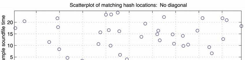
relative time sequence. The problem of deciding whether a match. Figure 2A illustrates a scatterplot of database time
match has been found reduces to detecting a significant versus sample time for a track that does not match the
cluster of points forming a diagonal line within the sample. There are a few chance associations, but no linear
scatterplot. Various techniques could be used to perform correspondence appears. Figure 3A shows a case where a
the detection, for example a Hough transform or otherFigure 5: Recognition rate -- Additive noise + GSM compression
100.00%
90.00%
80.00%
70.00%
60.00%
50.00%
40.00%
30.00%
20.00%
10.00%
0.00%
-15 -12 -9 -6 -3 0 3 6 9 12 15
Signal/Noise Ratio (dB)
15 sec GSM 10 sec GSM 5 sec GSM
significant number of matching time pairs appear on a
diagonal line. Figures 2B and 3B show the histograms of
the δtk values corresponding to Figures 2A and 3B. 3 Performance
This bin scanning process is repeated for each track in the 3.1 Noise resistance
database until a significant match is found. The algorithm performs well with significant levels of
noise and even non-linear distortion. It can correctly
Note that the matching and scanning phases do not make identify music in the presence of voices, traffic noise,
any special assumption about the format of the hashes. In dropout, and even other music. To give an idea of the
fact, the hashes only need to have the properties of having power of this technique, from a heavily corrupted 15
sufficient entropy to avoid too many spurious matches to second sample, a statistically significant match can be
occur, as well as being reproducible. In the scanning phase determined with only about 1-2% of the generated hash
the main thing that matters is for the matching hashes to be tokens actually surviving and contributing to the offset
temporally aligned. cluster. A property of the scatterplot histogramming
technique is that discontinuities are irrelevant, allowing
2.3.1 Significance immunity to dropouts and masking due to interference.
As described above, the score is simply the number of One somewhat surprising result is that even with a large
matching and time-aligned hash tokens. The distribution of database, we can correctly identify each of several tracks
scores of incorrectly-matching tracks is of interest in mixed together, including multiple versions of the same
determining the rate of false positives as well as the rate of piece, a property we call “transparency”.
correct recognitions. To summarize briefly, a histogram of
the scores of incorrectly-matching tracks is collected. The Figure 4 shows the result of performing 250 sample
number of tracks in the database is taken into account and a recognitions of varying length and noise levels against a
probability density function of the score of the highest- test database of 10000 tracks consisting of popular music.
scoring incorrectly-matching track is generated. Then an A noise sample was recorded in a noisy pub to simulate
acceptable false positive rate is chosen (for example 0.1% “real-life” conditions. Audio excerpts of 15, 10, and 5
false positive rate or 0.01%, depending on the application), seconds in length were taken from the middle of each test
then a threshold score is chosen that meets or exceeds the track, each of which was taken from the test database. For
false-positive criterion. each test excerpt, the relative power of the noise was
normalized to the desired signal-to-noise ratio, then linearly
added to the sample. We see that the recognition rate dropsto 50% for 15, 10, and 5 second samples at approximately
-9, -6, and -3 dB SNR, respectively Figure 5 shows the
same analysis, except that the resulting music+noise 5 References
mixture was further subjected to GSM 6.10 compression, [1] Avery Li-Chun Wang and Julius O. Smith, III., WIPO
then reconverted to PCM audio. In this case, the 50% publication WO 02/11123A2, 7 February 2002,
recognition rate level for 15, 10, and 5 second samples (Priority 31 July 2000).
occurs at approximately -3, 0, and +4 dB SNR. Audio [2] http://www.musiwave.com
sampling and processing was carried out using 8KHz, [3] Jaap Haitsma, Antonius Kalker, Constant Baggen, and
mono, 16-bit samples. Job Oostveen., WIPO publication WO 02/065782A1,
22 August 2002, (Priority 12 February, 2001).
[4] Jaap Haitsma, Antonius Kalker, “A Highly Robust
3.2 Speed Audio Fingerprinting System”, International
For a database of about 20 thousand tracks implemented on Symposium on Music Information Retrieval (ISMIR)
a PC, the search time is on the order of 5-500 milliseconds, 2002, pp. 107-115.
depending on parameters settings and application. The [5] Neuros Audio web site: http://www.neurosaudio.com/
service can find a matching track for a heavily corrupted [6] Sean Ward and Isaac Richards, WIPO publication WO
audio sample within a few hundred milliseconds of core 02/073520A1, 19 September 2002, (Priority 13 March
search time. With “radio quality” audio, we can find a 2001)
match in less than 10 milliseconds, with a likely [7] Audible Magic web site:
optimization goal reaching down to 1 millisecond per http://www.audiblemagic.com/
query. [8] Erling Wold, Thom Blum, Douglas Keislar, James
Wheaton, “Content-Based Classification, Search, and
3.3 Specificity and False Positives Retrieval of Audio”, in IEEE Multimedia, Vol. 3, No.
3: FALL 1996, pp. 27-36
The algorithm was designed specifically to target
[9] Clango web site: http://www.clango.com/
recognition of sound files that are already present in the
[10] Cheng Yang, “MACS: Music Audio Characteristic
database. It is not expected to generalize to live recordings.
Sequence Indexing For Similarity Retrieval”, in IEEE
That said, we have anecdotally discovered several artists in
Workshop on Applications of Signal Processing to
concert who apparently either have extremely accurate and
Audio and Acoustics, 2001
reproducible timing (with millisecond precision), or are
more plausibly lip synching.
The algorithm is conversely very sensitive to which
particular version of a track has been sampled. Given a
multitude of different performances of the same song by an
artist, the algorithm can pick the correct one even if they
are virtually indistinguishable by the human ear.
We occasionally get reports of false positives. Often times
we find that the algorithm was not actually wrong since it
had picked up an example of “sampling,” or plagiarism. As
mentioned above, there is a tradeoff between true hits and
false positives, and thus the maximum allowable
percentage of false positives is a design parameter that is
chosen to suit the application.
4 Acknowledgements
Special thanks to Julius O. Smith, III and Daniel P. W. Ellis
for providing guidance. Thanks also to Chris, Philip,
Dhiraj, Claus, Ajay, Jerry, Matt, Mike, Rahul, Beth and all
the other wonderful folks at Shazam, and to my Katja.You can also read