An Introduction to the Good, the Bad, & the Ugly Face Recognition Challenge Problem
←
→
Page content transcription
If your browser does not render page correctly, please read the page content below
An Introduction to the Good, the Bad, & the Ugly Face Recognition
                           Challenge Problem
               P. Jonathon Phillips, J. Ross Beveridge, Bruce A. Draper, Geof Givens, Alice J. O’Toole,
                David S. Bolme, Joseph Dunlop, Yui Man Lui, Hassan Sahibzada, and Samuel Weimer

   Abstract— The Good, the Bad, & the Ugly Face Challenge                               existing algorithms, nor so hard that progress cannot be
Problem was created to encourage the development of algo-                               made—the three bears problems [2].
rithms that are robust to recognition across changes that occur                            Traditionally, a challenge problem is specified by the two
in still frontal faces. The Good, the Bad, & the Ugly consists of
three partitions. The Good partition contains pairs of images                           sets of images that are to be compared. The difficulty of
that are considered easy to recognize. On the Good partition,                           the problem is then characterized by the performance of
the base verification rate (VR) is 0.98 at a false accept rate                           a set of algorithms tasked with matching the two sets of
(FAR) of 0.001. The Bad partition contains pairs of images of                           face images. To create a problem of a desired level of
average difficulty to recognize. For the Bad partition, the VR                           difficulty, a set of algorithms could be one component in
is 0.80 at a FAR of 0.001. The Ugly partition contains pairs
of images considered difficult to recognize, with a VR of 0.15                           the image selection process. Others factors in the selection
at a FAR of 0.001. The base performance is from fusing the                              process include limiting the number of images per person
output of three of the top performers in the FRVT 2006. The                             and requiring that pairs of images of a person are collected
design of the Good, the Bad, & the Ugly controls for pose                               on different days.
variation, subject aging, and subject “recognizability.” Subject                           The Good, the Bad, and the Ugly (GBU) challenge prob-
recognizability is controlled by having the same number of
images of each subject in every partition. This implies that the                        lem consists of three partitions which are called the Good, the
differences in performance among the partitions are result of                           Bad, and the Ugly. The difficulty of each partition is based
how a face is presented in each image.                                                  on the performance of three top performers in the FRVT
                                                                                        2006. The Good partition consists of pairs of face images
                          I. I NTRODUCTION                                              of the same person that are easy to match; the Bad partition
   Face recognition from still frontal images has made great                            contains pairs of face images of a person that have average
strides over the last twenty years. Over this period, error                             matching difficulty; and the Ugly partition concentrates on
rates have decreased by three orders of magnitude when                                  difficult to match face pairs. For the Good partition, the nom-
recognizing frontal faces in still images taken with consistent                         inal performance based on the FRVT 2006 is a verification
controlled illumination in an environment similar to a stu-                             rate (VR) of 0.98 at a false accept rate (FAR) of 0.001. For
dio [1], [2], [3], [4], [5], [6]. Under these conditions, error                         the Bad and Ugly partitions, the corresponding VR at a FAR
rates below 1% at a false accept rate of 1 in 1000 were                                 of 0.001 are 0.80 and 0.15. The performance range over the
reported in the Face Recognition Vendor Test (FRVT) 2006                                three partitions is roughly an order of magnitude. The three
and the Multiple Biometric Evaluation (MBE) 2010 [4], [6].                              partitions capture the range of performance inherent in less
   With this success, the focus of research is shifting to                              constrained images1 .
recognizing faces taken under less constrained conditions.                                 There are numerous sources of variation, known and
Less constrained conditions include allowing greater vari-                              unknown, in face images that can effect performance. Four
ability in pose, ambient lighting, expression, size of the                              of these factors are explicitly controlled in the design of
face, and distance from the camera. The trick in designing a                            the GBU challenge problem: subject aging, pose, change
face recognition challenge problem is selecting the degree                              in camera, and variations among faces. The data collection
to which the constraints are relaxed so that the resulting                              protocol eliminated or significantly reduced the impact of
problem has the appropriate difficulty. The complexity of                                three of the factors. Changes in the appearance of a face due
this task is compounded by the fact that it is not well                                 to aging is not a factor because all images were collected in
understood how the above factors effect performance. The                                the same academic year. However, the data set contains the
problem cannot be too easy that it is an exercise in tuning                             natural variations in a person’s appearance that would occur
                                                                                        over an academic year. Because all the images were collected
   P. J. Phillips and H. Sahibzada are with the National Institute of Standards
and Technology, 100 Bureau Dr., MS 8940 Gaithersburg MD 20899, USA                      by the same model of camera, difference in performance
(e-mail: jonathon@nist.gov). Please direct correspondence to P. J. Phillips.            cannot be attributable to changes in the camera. Changes in
   J. R. Beveridge, B. A. Draper, D. S. Bolme, and Y-M Lui are with                     pose are not a factor because the data set consists of frontal
the Department of Computer Science, Colorado State U., Fort Collins, CO
46556, USA.                                                                             face images.
   G. Givens is with the Department of Statistics, Colorado State U., Fort                 One potential source of variability in performance is that
Collins, CO 46556, USA.
   A. J. OToole, J. Dunlop, and S. Weimer are with the School of Behavioral                1 Instructions for obtaining the complete GBU distribution can be found
and Brain Sciences, GR4.1 The University of Texas at Dallas Richardson,                 at http://face.nist.gov. Instructions for obtaining the LRPCA algorithm can
TX 75083-0688, USA                                                                      be found at http://www.cs.colostate.edu/facerec.
                                                                                  346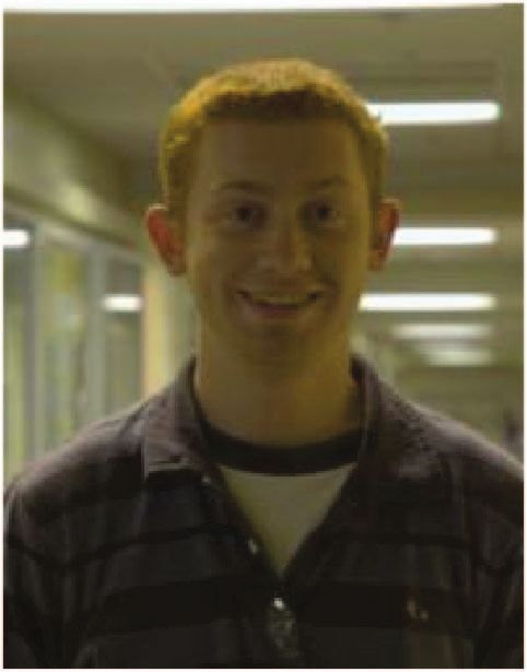
people vary in their “recognizability.” To control for this After applying these constraints, and given the total number
source of variability, the face images of the same people are of images available, the number of images per person in the
in each partition. In addition, each partition has the same target and query sets was selected to fall between 1 and 4.
number of images of each person. Because the partition This number depended upon the total availability of images
design controls for variation in the recognizability of faces, for each person.
the differences in performance among the three partitions are The selection criteria for the partition results in the follow-
a result of how a face is presented in each image, and with ing properties. An image is only in one partition. There are
the pairs of faces that are matched. the same number of match face pairs in each partition and the
same number of non-match pairs between any two subjects.
II. G ENERATION OF THE G OOD , THE BAD , & THE U GLY This implies that any difference in performance between the
PARTITIONS partitions is not a result of different people. The difference
in performance is a result of the different conditions under
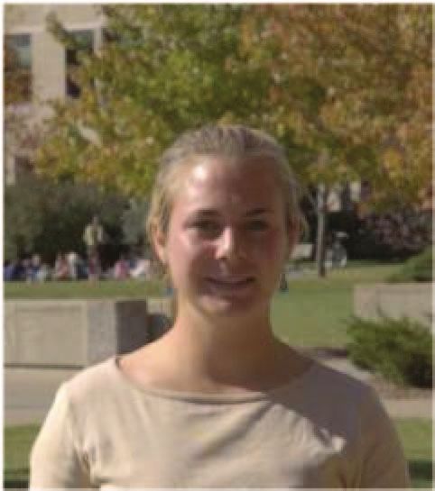
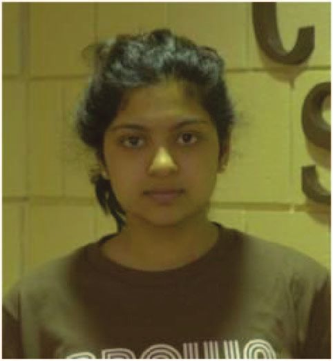
The GBU partitions were constructed from the Notre which the images were acquired. Figures 1, 2, and 3, are
Dame multi-biometric data set used in the FRVT 2006 [4]. examples of matching face pairs from each of the partitions.
The images for the partitions were selected from a superset of The images included in the GBU target and query sets
9,307 images of 570 subjects. All the images in the superset were decided independently for each person. For each subject
are frontal still face images collected either outside or with i, a subject-specific similarity matrix Si is extracted from a
ambient lighting in hallways. The images were acquired with larger matrix containing similarity scores from the FRVT
a 6 Mega-pixel Nikon D70 camera. All photos were taken 2006 fusion algorithm. Each subject-specific matrix contains
in the 2004-2005 academic year (Aug 2004 through May all similarity scores between pairs of images of subject i. For
2005). the Good partition, a greedy selection algorithm iteratively
Each partition in the GBU is specified by two sets of added match face pairs for subject i that maximized the
images, a target set and a query set. For each partition, an average similarity score for subject i; for the Ugly partition,
algorithm computes a similarity score between all pairs of match face pairs were selected to minimize the average
images in that partition’s target and query sets. A similarity similarity score for subject i; and for the Bad partition, face
score is a measure of the similarity between two faces. pairs for subject i were selected to maintain an approximately
A higher similarity scores implies greater likelihood that average similarity score. The selection process for each
the face images are of the same person. If an algorithm subject was repeated until the desired number of images were
reports a distance measure, then a smaller distance measure selected for that subject. Since the images for each subject
implies greater likelihood that the face images are of the are selected independently, the similarity score associated
same person. A distance measure is converted to a similarity with a good face pair can vary from subject to subject
score by multiplying by minus one. The set of all similarity (similarly for the Bad and Ugly partitions).
scores between a target and a query set is called a similarity Each of the GBU target and query sets contains 1,085
matrix. A pair of face images of the same person is called a images for 437 distinct people. The distribution of image
match pair; and a pair of face images of different people counts per person in the target and query sets are 117 subjects
is called a non-match pair. From the similarity matrix, with 1 image; 122 subjects with 2 images; 68 subjects with
receiver operating characteristics (ROC) and other measures 3 images; and 130 subjects with 4 images. In each partition
of performance can be computed. there is 3,297 match face pairs and 1,173,928 non-match face
To construct the GBU Challenge Problem we sought to pairs. In the GBU image set 58% of the subjects were male
specify target and query sets for each of the three partitions and 42% female; and 69% of the subjects were Caucasian,
such that recognition difficulty would vary markedly while at 22% east Asian, 4% Hispanic, and the remaining 5% other
the same time factors such as the individual people involved groups; and 94% of the subjects were between 18 and 30
or number of images per person remained the same. To gauge years old with the remaining 6% over 30 years old. For the
the relative difficulty associated with recognizing a pair of images in the GBU, the average distance between the centers
images, similarity scores were created by fusing scores from of the eyes is 175 pixels with a standard deviation of 36
three of the top performing algorithms in the FRVT 2006; pixels.
this fusion process is described more fully in the next section.
III. T HE FRVT 2006 F USION P ERFORMANCE
The following constraints were imposed when selecting
the GBU partitions: Performance results for the GBU Challenge Problem are
Distinct Images: An image can only be in one reported for the GBU FRVT 2006 fusion algorithm, which is
target or query set. a fusion of three of the top performers in the FRVT 2006. The
algorithms were fused in a two-step process. In the first step,
Balanced subject counts: The number of images
for each algorithm, the median and the median absolute devi-
per person are the same in all target
ation (MAD) were estimated from every 1 in 1023 similarity
and query sets.
scores (mediank and MADk are the median and MAD for
Different days: The images in all match pairs were algorithm k). The median and MAD were estimated from 1
taken on different days. in 1023 similarity scores to avoid over tuning the estimates to
347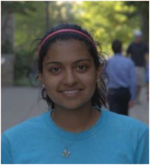
(a)                                      (b)                                     (c)
Fig. 1.   Examples of face pairs of the same person from each of the partitions: (a) good, (b) challenging, and (c) very challenging.

                        (a)                                      (b)                                     (c)
Fig. 2.   Examples of face pairs of the same person from each of the partitions: (a) good, (b) challenging, and (c) very challenging.

                                                                 348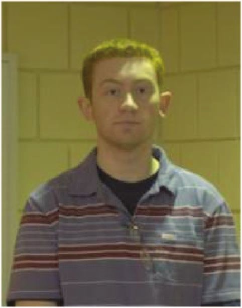
(a)                                      (b)                                     (c)
        Fig. 3.   Examples of face pairs of the same person from each of the partitions: (a) good, (b) challenging, and (c) very challenging.

the data. The similarity scores were selected to evenly sample                 there are images of the subjects in the GBU problem that are
the images in the experiment. The fused similarity scores are                  in the FRGC and the MBGC data sets. These images must
the sum of the individual algorithm similarity scores after the                be excluded from model selection, training, or tuning of an
median has been subtracted and then divided by the MAD.                        algorithm.
If sk is a similarity score for
                              algorithm k and sf is a fusion                     We illustrate acceptable and unacceptable training proto-
similarity score, then sf = k (sk − mediank )/MADk .                           cols with three examples. The first example is training of a
   Figure 4 reports performance of the fusion algorithm on                     principal components analysis (PCA) based face-recognition
each of the partitions. Figure 5 shows the distribution of                     algorithm. In a PCA-based algorithm, PCA is performed
the match and non-matches for the fusion algorithm on all                      on a training set to produce a set of Eigenfaces. A face is
three partitions. The non-match distribution is stable across                  represented by projecting a face image on the set of Eigen-
all three partitions. The match distribution shifts for each                   faces. To meet the training requirements of the protocol,
partition. The Good partition shows the greatest difference                    images of subjects in the GBU must be excluded from the
between the median of the match and non-match distributions                    PCA decomposition that produces a set of Eigenfaces. The
and the least difference for the Ugly partition.                               benchmark algorithm in Section V includes a training set
                          IV. P ROTOCOL                                        that satisfies the training protocol.
   The protocol for the GBU Challenge Problem is one-                             A second example is taken from a common training
to-one matching with training, model selection, and tuning                     procedure for linear discriminant analysis (LDA) in which
completed prior to computing performance on the partitions.                    the algorithm is trained on the images in a target set. Training
Consequently, under this protocol, the similarity score s(t, q)                an algorithm on a GBU target set the GBU protocol. Gen-
between a target image t and a query image q does not in                       erally, it is well known that the performance of algorithms
any way depend on the other images in the target and query                     can improve with such training, but the resulting levels of
sets. Avoiding hidden interactions between images, other                       performance typically do not generalize. For example, we’ve
than the two being compared at the moment, provides the                        conducted experiments with an LDA algorithm trained on
clearest picture of how algorithms perform. More formally,                     the GBU target images and performance improved over the
any approach that redefines similarity s(t, q; T ) such that                    baseline algorithm presented, see Section V. However, when
it depends upon the target (or query) image set T is NOT                       we trained our LDA algorithm following the GBU protocol,
allowed in the GBU Challenge Problem.                                          performance did not match the LDA algorithm trained on a
   To maintain separation of training and test sets, an algo-                  GBU target set.
rithm cannot be trained on images of any of the subjects                          The GBU protocol does permit image specific representa-
in the GBU Challenge Problem. It is important to note that                     tions as long as the representation does not depend on other
                                                                         349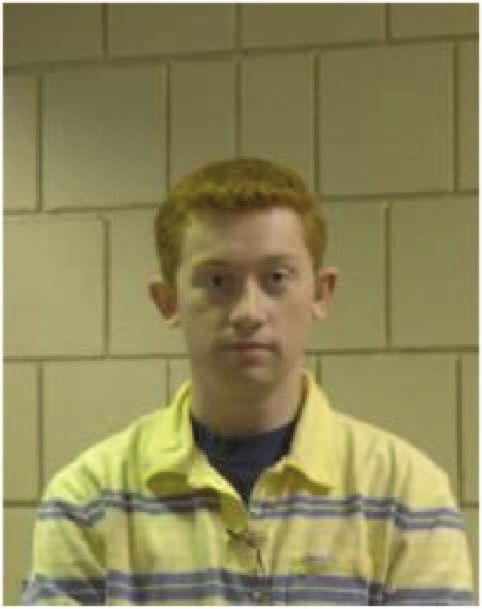
Good                                                 Bad                                           Ugly

                                  Less
                     Similarity
                                  More

                                                Match                 Nonmatch                 Match                       Nonmatch                Match                 Nonmatch

                                     0.1                0.0     0.1          0.2     0.3 0.1           0.0           0.1          0.2    0.3 0.1           0.0     0.1          0.2   0.3

Fig. 5. Histogram of the match and non-match distributions for the Good, the Bad, & the Ugly partitions. The green bars represent the match distribution
and the yellow bars represent the non-match distribution. The horizontal axes indicate relative frequency of similarity scores.

                                                                                                                         set and consequently is permitted by the GBU protocol.
                                                                                                                                          V. BASELINE A LGORITHM
                     1.0

                                           G
                                               0.98                                                                         The GBU Challenge Problem includes a baseline face
                                                                                                                         recognition algorithm as an entry point for researchers. The
                                                                                                                         baseline serves two purposes. First, it provides a working
                     0.8

                                           G
                                               0.80
                                                                                                                         example of how to carry out the GBU experiments following
                                                                                                                         the protocol. This includes training, testing and evaluation
                                                                                                                         using ROC analysis. Second, it provides a performance stan-
 Verification rate
                     0.6

                                                                                                                         dard for algorithms applied to the GBU Challenge Problem.
                                                                                                                            The architecture of the baseline algorithm is a refined im-
                                                                                                                         plementation of the standard PCA-based face recognition al-
                     0.4

                                                                                                                         gorithm, also known as Eigenfaces [7][8]. These refinements
                                                                                                                         considerably improve performance over a standard PCA-
                                                                                                                         based implementation. The refinements include representing
                     0.2

                                           G
                                                                                                                         a face by local regions, a self quotient normalization step,
                                               0.15
                                                                                                   Good                  and weighting eigenfeatures based on Fischer’s criterion. We
                                                                                                   Bad                   refer to the GBU baseline algorithm as local region PCA
                     0.0

                                                                                                   Ugly
                                                                                                                         (LRPCA).
                                    0.001                      0.01                0.1                       1.0            It may come as a surprise to many in the face recognition
                                                                 False accept rate                                       community that a PCA-based algorithm was selected for the
                                                                                                                         GBU benchmark algorithm. However, when developing the
                                                                                                                         LRPCA baseline algorithm, we explored numerous standard
Fig. 4. ROC for the Fusion algorithm on the Good, the Bad, & the Ugly
partitions. The verification rate for each partition at a FAR of 0.001 is                                                 alternatives, including LDA-based algorithms and algorithms
highlighted by the vertical line at FAR=0.001.                                                                           combining Gabor based features with kernel methods and
                                                                                                                         support vector machines. For performance across the full
                                                                                                                         range of the GBU Challenge Problem, our experiments
                                                                                                                         with alternative architectures never resulted in overall per-
images of other subjects in the GBU Challenge Problem.                                                                   formance better than the GBU baseline algorithm.
An example is an algorithm based on person-specific PCA
representations. In this example, during the geometric nor-                                                              A. A Step-by-step Algorithm Description
malization process, 20 slightly different normalized versions                                                               The algorithm’s first step is to extract a cropped and
of the original face would be created. A person-specific PCA                                                              geometrically-normalized face region from an original face
representation is generated from the set of 20 normalized                                                                image. The original image is assumed to be a still image and
face images. This method conforms with the GBU training                                                                  the pose of the face is close to frontal. The face region in the
protocol because the 20 face images and the person specific                                                               original is scaled, rotated, and cropped to a specified size and
PCA representation are functions of the original single face                                                             the centers of the eyes are horizontally aligned and placed on
image. When there are multiple images of a person in a target                                                            standard pixel locations. In the baseline algorithm, the face
or query set, this approach will generate multiple image-                                                                chip is 128 by 128 pixels with the centers of the eyes spaced
specific representations. This training procedure does not                                                                64 pixels apart. The baseline algorithm runs in two modes:
introduce any dependence upon other images in the target                                                                 partially and fully automatic. In the partially automatic mode
                                                                                                                   350
1.0
                                                                                                           0.8
                                                                                                                   G

                                                                                       Verification rate
                                                                                                                       0.64

                                                                                                           0.6
                                                                                                           0.4
                                                                                                                   G
                                                                                                                       0.24

                                                                                                           0.2
                                                                                                                                                      Good
                                                                                                                   G
                                                                                                                       0.07                           Bad

                                                                                                           0.0
                                                                                                                                                      Ugly
Fig. 6. This figure shows a cropped face and the thirteen local regions. The
crop face has been geometrically normalized and the self quotient procedure                                      0.001        0.01             0.1       1.0
performed.                                                                                                                      False accept rate

                                                                                      Fig. 8. ROC for the LRPCA baseline algorithm on the GBU partitions.
                                                                                      The verification rate for each partition at a FAR of 0.001 is highlighted by
                                                                                      the vertical line at FAR=0.001.

                                                                                      in the GBU Challenge Problem. A region in a face is encoded
                                                                                      by the 250 coefficients computed by projecting the region
Fig. 7. This figure illustrates the computation of a self-quotient face image.
The face image to the left is a cropped and geometrically normalized image.           onto the region’s 250 eigenvectors. A face is encoded by
The image in the middle is the geometrically normalized image blurred by a            concatenating the the 250 coefficients for each of the 14
Gaussian kernel. The image on the left is a self-quotient image. This image           regions into a new vector of length 3500.
is obtained by pixel-wise division of the normalized image by the blurred
image.                                                                                   Each dimension in the PCA subspace is further scaled.
                                                                                      First, the representation is whitened by scaling each dimen-
                                                                                      sion to have a sample standard deviation of one on the
the coordinates of the centers of the eyes are provided; in                           training set. Next, the weight on each dimension is further
the fully automatic mode, the centers of the eyes are located                         adjusted based on Fisher’s criterion. This weight is computed
by the baseline algorithm.                                                            based on the images in the training set. The Fisher’s criterion
   In the LRPCA algorithm, the PCA representation is based                            weight emphasizes the dimensions along which images of
on thirteen local regions and the complete face chip. The                             different people are spread apart. The weight attenuates
thirteen local regions are cropped out of a normalized face                           the dimensions along which the average distance between
image. Some of the local regions overlap, see Figure 6. The                           images of the same person and images of different people
local regions are centered relative to the average location of                        are roughly the same.
the eyes, eyebrows, nose and mouth.                                                      When used for recognition, i.e. during testing, images are
   The next step normalizes the 14 face regions to attenuate                          first processed as described above and then projected into
variation in illumination. First, self quotient normalization is                      the 14 distinct PCA subspaces associated with each of the
independently applied to each of the 14 regions [9]. The self                         14 regions. The coordinates of images projected into these
quotient normalization procedure first smoothes each region                            spaces, 250 for each of the 14 regions, are then concatenated
by convolving it with a two-dimensional Gaussian kernel and                           into a single feature vector representing the appearance
then divides the original region by the smoothed region, see                          of that face. This produces one vector per face image;
Figure 7. In the final normalization step, the pixel values in                         each vector contains 3,500 values. The baseline algorithm
each region are further adjusted to have a sample mean of                             measures similarity between pairs of faces by computing
zero and a sample standard deviation of one.                                          the Pearson’s correlation coefficient between pairs of these
   During training, 14 distinct PCA subspaces are con-                                vectors. The performance of the baseline algorithm on the
structed, one for each of the face regions. From each PCA de-                         GBU Challenge Problem is summarized in Figure 8. A
composition, the 3rd through 252th eigenvectors are retained                          comparison of performance of the Fusion and the LRPCA-
to represent the face. The decision to use these eigenvectors                         baseline algorithm is given in Table I.
was based upon experiments on images similar to the images                               A recent area of interest in face recognition and bio-
                                                                                351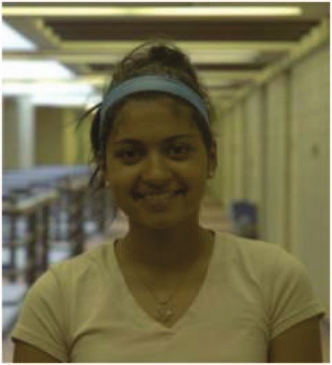
metrics is recognition from the ocular region of the face.                in pairs. Additional possible lines of investigation include
There is interest in recognition from both near infrared and              understanding the factors that characterize the difference in
visible imagery. The region-based design of the LRPCA                     match face pairs across the partitions. A second line of re-
algorithm allows for baselining ocular performance on the                 search is characterizing the recognizability of a face; e.g., the
GBU partitions. Baseline performance for the left ocular is               biometric zoo. A third line of research is developing methods
computed from three of the 14 regions. The regions are                    for predicting performance of face recognition algorithms.
the left eye and two left eye brow regions. For the right                 The design of the GBU Challenge Problem encourages both
ocular region, performance is computed from the right eye                 the development of algorithms, and the investigation of
and two right eye brow regions. The left eye (resp. right                 methods for understanding algorithm performance.
eye) are with respective to the subject; e.g., the left ocular
                                                                                                  ACKNOWLEDGMENTS
region corresponds to a subject left eye. Performance for the
LRPCA-ocular baseline for the left and right ocular regions                  The authors wish to thank the Federal Bureau of Inves-
is given in Figure 9.                                                     tigation (FBI) and the Technical Support Working Group
   A summary of performance of the Fusion, the LRPCA-                     (TSWG) for their support of this work. The identification
face baseline and the LRPCA-ocular baseline algorithms are                of any commercial product or trade name does not imply
given in Table I.                                                         endorsement or recommendation by the Colorado State Uni-
                                                                          versity, the National Institute of Standards and Technology
                              TABLE I                                     or the University of Texas at Dallas. The authors thank Jay
P ERFORMANCE OF THE F USION , THE LRPCA- FACE BASELINE AND THE            Scallan for his assistance in preparing the GBU challenge
    LRPCA- OCULAR     BASELINE ALGORITHMS .   F OR THE OCULAR             problem.
  BASELINE , PERFORMANCE IS GIVEN FOR BOTH THE LEFT AND THE
 RIGHT OCULAR REGIONS .   T HE VERIFICATION RATE AT A FAR = 0.001                                       R EFERENCES
                              IS GIVEN .                                   [1] P. J. Phillips, H. Wechsler, J. Huang, and P. Rauss, “The FERET
                                                                               database and evaluation procedure for face-recognition algorithms,”
                                            LRPCA-ocular                       Image and Vision Computing Journal, vol. 16, no. 5, pp. 295–306,
         Partition   Fusion   LRPCA-face    left  right                        1998.
          Good        0.98       0.64       0.47  0.46                     [2] P. J. Phillips, H. Moon, S. Rizvi, and P. Rauss, “The FERET evaluation
           Bad        0.80       0.24       0.16  0.17                         methodology for face-recognition algorithms,” IEEE Trans. PAMI,
          Ugly        0.15       0.07       0.05  0.05                         vol. 22, pp. 1090–1104, October 2000.
                                                                           [3] P. J. Phillips, P. J. Flynn, T. Scruggs, K. W. Bowyer, J. Chang,
                                                                               K. Hoffman, J. Marques, J. Min, and W. Worek, “Overview of the face
                                                                               recognition grand challenge,” in IEEE Computer Society Conference
                                                                               on Computer Vision and Pattern Recognition, 2005, pp. 947–954.
            VI. D ISCUSSION AND C ONCLUSION                                [4] P. J. Phillips, W. T. Scruggs, A. J. O’Toole, P. J. Flynn, K. W. Bowyer,
                                                                               C. L. Schott, and M. Sharpe, “FRVT 2006 and ICE 2006 large-scale
   This paper introduces the Good, the Bad, & the Ugly                         results,” IEEE Trans. PAMI, vol. 32, no. 5, pp. 831–846, 2010.
Challenge Problem. The main goal of the challenge is to                    [5] P. J. Phillips, P. J. Flynn, J. R. Beveridge, W. T. Scruggs, A. J. O’Toole,
encourage the development of algorithms that are robust                        D. Bolme, K. W. Bowyer, B. A. Draper, G. H. Givens, Y. M. Lui,
                                                                               H. Sahibzada, J. A. Scallan III, and S. Weimer, “Overview of the
to recognizing frontal faces taken outside of studio style                     Multiple Biometrics Grand Challenge,” in Proceedings Third IAPR
image collections. The three partitions in the GBU Challenge                   International Conference on Biometrics, 2009.
Problem emphasize the range of performance that is possible                [6] P. J. Grother, G. W. Quinn, and P. J. Phillips, “MBE 2010: Report on
                                                                               the evaluation of 2D still-image face recognition algorithms,” National
when comparing faces photographed under these conditions.                      Institute of Standards and Technology, NISTIR 7709, 2010.
This structure allows for researchers to concentrate on the                [7] M. Turk and A. Pentland, “Eigenfaces for recognition,” J. Cognitive
“hard” aspects of the problem while not compromising                           Neuroscience, vol. 3, no. 1, pp. 71–86, 1991.
                                                                           [8] M. Kirby and L. Sirovich, “Application of the karhunen-loeve pro-
performance on the “easier” aspects.                                           cedure for the characterization of human faces,” IEEE Trans. PAMI,
   Partitioning the challenge by levels of difficulty is the most               vol. 12, no. 1, pp. 103–108, 1990.
prominent feature of the GBU Challenge Problem design.                     [9] H. Wang, S. Li, Y. Wang, and J. Zhang, “Self quotient image for
                                                                               face recognition,” in Proceedings, International Conference on Image
Another is controlling for the “recognizability” of people by                  Processing, vol. 2, 2004, pp. 1397–1400.
selecting images of the same 437 people for inclusion in                  [10] A. J. O’Toole, P. J. Phillips, X. An, and J. Dunlop, “Demographic
each of the GBU partitions. The data in the three partitions                   effects on estimates of automatic face recognition performance,” in
                                                                               Proceedings, Ninth International Conference on Automatic Face and
is further balanced so as to ensure that for each person                       Gesture Recognition, 2011.
the number of target and query images in each partition                   [11] J. R. Beveridge, P. J. Phillips, G. H. Givens, B. A. Draper, M. N. Teli,
is the same. The design of the GBU Challenge Problem                           and D. S. Bolme, “When high-quality face images match poorly,” in
                                                                               Proceedings, Ninth International Conference on Automatic Face and
means that any difference in performance observed between                      Gesture Recognition, 2011.
partitions cannot be attributed to differences between people
or numbers of images for individual people.
   The unique design of the GBU Challenge Problem al-
lows researchers to investigate factors that influence the
performance of algorithms. O’Toole et al. [10] looks at the
demographic effects on the nonmatch distribution. Beveridge
et al. [11] shows that the quality of face images comes
                                                                    352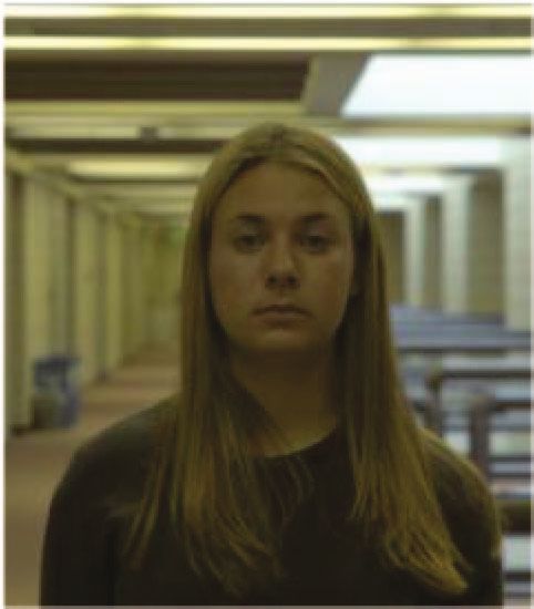
1.0

                                                                                                          1.0
                       0.8

                                                                                                          0.8
   Verification rate

                                                                                      Verification rate
                       0.6

                                                                                                          0.6

                               G
                                   0.47                                                                           G
                                                                                                                      0.46
                       0.4

                                                                                                          0.4
                       0.2

                                                                                                          0.2

                                                                                                                  G
                               G
                                   0.16                                                                               0.17
                                                                   Good                                                                              Good
                               G                                   Bad                                            G                                  Bad
                                   0.05                                                                               0.05
                       0.0

                                                                                                          0.0

                                                                   Ugly                                                                              Ugly

                             0.001        0.01             0.1        1.0                                       0.001        0.01             0.1       1.0
                                            False accept rate                                                                  False accept rate

                                                 (a)                                                                                (b)

Fig. 9. ROC for the LRPCA-ocular baseline algorithm on the Good, the Bad, & the Ugly partitions. In (a) performance is for the left ocular region that
consists of the left eye and two left eye-brow regions; performance in (b) is for corresponding right ocular regions. The verification rate for each partition
at a FAR of 0.001 is highlighted by the vertical lines at FAR=0.001.

                                                                            353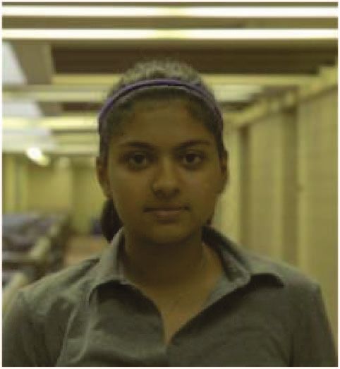
You can also read