Analysing the impact of dependency on conditional survival functions using copulas
←
→
Page content transcription
If your browser does not render page correctly, please read the page content below
STATISTICS IN TRANSITION new series, March 2021
Vol. 22, No. 1, pp. 217–226, DOI 10.21307/stattrans-2021-013
Received – 17.07.2020; accepted – 06.11.2020

       Analysing the impact of dependency on conditional
                survival functions using copulas
                       Hadi Safari-Katesari1 , Samira Zaroudi2
                                             ABSTRACT
     Nowadays, insurance contract reserves for coupled lives are considered jointly, which has a
     significant influence on the process of determining actuarial reserves. In this paper, condi-
     tional survival distributions of life insurance reserves are computed using copulas. Subse-
     quently, the results are compared with an independence case. These calculations are based
     on selected Archimedean copulas and apply when the ‘death of one individual’ condition
     exists. The estimation outcome indicates that the insurer reserves calculated by means of
     Archimedean copulas are far more effective than those resulting from an independence as-
     sumption. The study demonstrates that copula-based dependency modelling improves the
     calculations of reserves made for actuarial purposes.
     Key words: conditional survival distribution, copula, Kendall’s tau, reserves, life table.

1. Introduction
    There exist extensive literature on modelling insurance contracts of two lives using the
independence assumption between two lives with focusing on the starting time of the con-
tracts. The main problem for calculating reserves (provisions) between two lifetimes is
finding a way to reduce costs of insurance companies. In this paper, we relax the indepen-
dence assumption and show that the dependency between two lives has a great effect on the
solvency of financial businesses such as insurance companies.
    In the past few years, many works have been done on application of copula for modelling
the dependency between two lifetimes. See, for example Hougaard (2000), Spreeuw (2006),
Spreeuw and Owadally (2013), and Zaroudi et al. (2018a,b). Lee et al. (2014) studied the
dependence between the policyholders in multiple-life of insurance contracts. Also, many
works considered the relationship between two lifetimes of coupled lives, such as Carriere
(2000) and Ji et al. (2011). This dependency has a significant impact on the determination
of pricing of the insurance contracts. If one considers remaining lifetimes of coupled lives
dependently at the beginning period of issuing the insurance policy, then the death chance
of two lives might depend on the life status of each of them. A copula is a useful tool
for building multivariate distributions when the marginal distributions are available. The
copula captures the linear and nonlinear dependencies available in dataset simultaneously
and is an applicable tool for modelling the dependency structures between different random
   1 Corresponding Author: School of Mathematical and Statistical Sciences, Southern Illinois University, Car-

bondale, IL 62901-4408, USA. E-mail: hadi.safari@siu.edu. ORCID: https://orcid.org/0000-0003-2630-3133.
   2 School of Mathematical and Statistical Sciences, Southern Illinois University, Carbondale, IL 62901-4408,

USA. ORCID: https://orcid.org/0000-0001-8290-6137.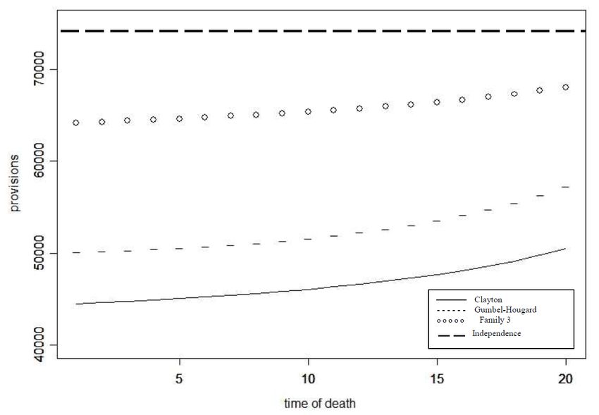
218                            H. Safari-Katesari, S. Zaroudi: Analysing the impact of dependency ...

variables (r.v.’s). Moreover, it opens a new vision for considering the properties of joint
distributions of marginal r.v.’s such that it separates the study of dependency effects from
the effects of the margins (Mari and Kotz, 2004). Following the studies by Spreeuw and
Owadally (2013), and Spreeuw (2006), in this paper, we discuss methods of calculating the
insurer’s reserves based on copula models using the life table of France. Moreover, we apply
Kendall’s tau for measuring the dependency of variables using copula models. Our method
is useful by selecting an optimal copula and bringing an approach for reserves calculation
of contracts. Statistical analyses were performed with R version 3.6.2: The R Project for
Statistical Computing.
    The framework of this paper goes as follows: In Section 2, we review copula models,
family of Archimedean copulas, Kendall’s tau correlation coefficient, survival functions,
and the relationship between copula and survival functions based on ‘death of one individ-
ual’. In Section 3, we calculate reserves for life insurance policy and three Archimedean
copulas for ‘death of one individual’ using life table of France. In Section 4, we apply a
numerical example for reserves of two lifetimes in insurance contracts. Section 5 provides
conclusion remarks.

2. Copula
    The term copula is a Latin word ‘copuler’ which means ‘tie and link’ and was intro-
duced at first by Sklar Theorem (Sklar, 1959) describing the relationship between r.v.’s to
build multivariate distribution functions (Nelsen, 2006). In this paper, only bivariate copu-
las are used for considering the dependency of two lives when one of them dies during the
time period of the insurance contract. In the next subsection, the bivariate copulas are intro-
duced and their properties are investigated. For more information on properties of copula in
insurance and financial concept, see Frees and Valdez (1998), Katesari and Vajargah (2015),
Katesari and Zarodi (2016), and Safari-Katesari and Zaroudi (2020).

2.1. Random Variables and Copula
    Copula is a statistical tool for modelling the dependence between r.v.’s. Let us start with
the definition of copula from Denuit et al. (2005) as follows:
Definition 2.1 A bivariate copula C : [0, 1]2 → [0, 1] is a non-decreasing and right-continuous
function which preserves the following:
   1. lim C(u1 , u2 ) = 0, for i = 1, 2,
       ui →0

   2. lim C(u1 , u2 ) = u1 and lim C(u1 , u2 ) = u2 ,
       u2 →1                       u1 →1

   3. C(v1 , v2 ) −C(u1 , v2 ) −C(v1 , u2 ) +C(u1 , u2 ) ≥ 0,
for any u1 , u2 , v1 , v2 ∈ [0, 1], u1 ≤ v1 and u2 ≤ v2 .
By Sklar’s Theorem (Sklar, 1959), one can easily consider the dependence between mul-
tivariate distribution functions and their corresponding margins with copulas. Now, we
consider Sklar’s Theorem, which is as follows: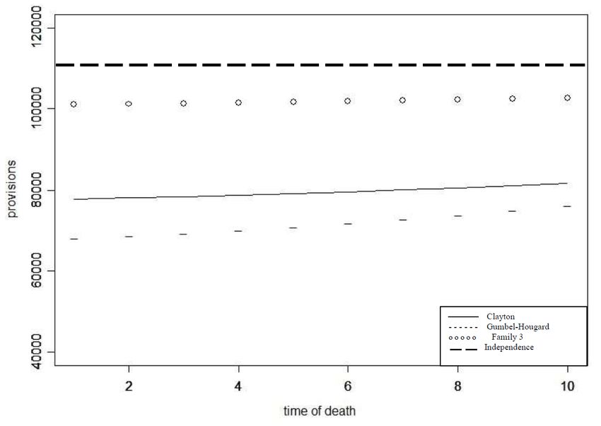
STATISTICS IN TRANSITION new series, March 2021 219
Theorem 2.1 Consider the joint distribution HX (x1 , x2 ) with continuous marginal cumu-
lative distribution functions (CDFs) F1 and F2 . Then, a copula C is available for all
x1 , x2 ∈ [−∞, +∞] as follows:
HX (x1 , x2 ) = C(F1 (x1 ), F2 (x2 )). (1)
Conversely, the function HX denoted in Eq. (1) is a bivariate distribution function when C
is a copula function with marginal CDFs F1 and F2 .
Moreover, we use the following corollary and definition from Nelsen (2006) and Denuit et
al. (2005), respectively.
Corollary 2.1 Following Theorem 2.1, for any (u1 , u2 ) ∈ [0, 1]2 , we have:
C(u1 , u2 ) = HX (F1−1 (u1 ), F2−1 (u2 )).
Definition 2.2 For any (u1 , u2 ) ∈ [0, 1]2 , C(u1 , u2 ) = u1 u2 defined as the independent cop-
ula.
In what follows, we will introduce one of the most famous family of copulas named Archimedean
copulas.
2.2. Archimedean Copulas
The copula described by Genest and MacKay (1986a) and Genest and MacKay (1986b)
called the Archimedean copulas and there exist rich applications of this copula family in
the mathematical and statistical literature. Many actuarial and financial dataset have been
analyzed using Archimedean copulas; for more information, see Frees and Valdez (1998),
Denuit et al. (2005) and Klugman and Parsa (1999). One of the important features of
this family is that they are parametric. A generating function is the general structure of
Archimedean copula, which is introduced in the following definition from Denuit et al.
(2005).
Definition 2.3 Assume φ : [0, 1] → [0, +∞] is a continuous, strictly decreasing function and
has following characteristics:
0 00
φ (1) = 0, φ (τ) < 0, φ (τ) > 0, ∀τ ∈ (0, 1). (2)
Then, the bivariate copula
−1
φ (φ (u1 ) + φ (u2 )), if φ (u1 ) + φ (u2 ) ≤ φ (0),
Cφ (u1 , u2 ) = (3)
0, otherwise.
is generated by φ (·) defined in Eq. (2) where the copula Cφ (u1 , u2 ) is the Archimedean
copula for 0 ≤ u1 , u2 ≤ 1. The generator function of the copula is φ .220 H. Safari-Katesari, S. Zaroudi: Analysing the impact of dependency ...
One of the most important criteria for explaining the relationship between the dependency
and the Archimedean copula is expressed in the following Theorem from Nelsen (2006).
Theorem 2.2 Consider X and Y as r.v.’s with Archimedean copula C generated by φ . Then,
Kendall’s tau (τ) correlation for X and Y is as follows:
Z 1
φ (t)
τ = 1+4 0 dt. (4)
0 φ (t)
In this paper, we apply three copula functions in the Archimedean family, which are defined
in Table 1. In this table, the second column displays the values of dependence parameter
(θ ) indicating the case of independence, the third column shows the relationships between
θ and τ, and the fourth and fifth columns display generation functions and domains of θ for
these copulas, respectively (Nelsen, 2006).
Table 1: Three copulas in Archimedean copula family
Family Independence τ φ (τ) θ∈
Family 3 θ =0 (1/θ ) − e exp[τ −θ ] − e (0, ∞)
G-H θ =1 θ − 1/θ (− ln τ)θ [−1, ∞)
Clayton θ =0 θ /(θ + 2) τ −θ − 1 [−1, ∞)\{0}
2.3. Survival Function and Copula
A contract of life insurance defines on couple (two persons) lives with x and y ages
at time 0, respectively. The remaining lifetimes of persons x and y are defined by Tx
and Ty , where the marginal survival functions and the copula survival function are denoted
by STx (s1 ), STy (s2 ) and STx ,Ty (s1 , s2 ), respectively. The survival function of the remaining
lifetime at time t for the person aged x, given the death of person aged y at time ty is defined
as (Spreeuw, 2006):
− dtdy P(Tx > t + s, Ty > ty )
STx ;t (s|Ty = ty ) = P(Tx > t + s|Tx > t, Ty = ty ) =
− dtdy P(Tx > t, Ty > ty )
(5)
− dtdy STx ,Ty (t + s,ty ) (C2 (STx (t + s) , ξ ))ξ =ST (ty )
y
= = .
− dtdy STx ,Ty (t,ty ) (C2 (STx (t) , ξ ))ξ =ST (ty )
y
Notice that the function defined in Eq. (5) is a survival copula function where the partial
derivative of copula C for the second argument denoted with C2 such that C2 (STx (t) , ξ ) 6= 0
is defined for ξ = STy (ty ). Then, following Spreeuw (2006) and using Eq. (3), we have:
C(STx (t + s), STy (ty )) = φ −1 (φ (STx (t + s)) + φ (STy (ty ))) = STx ,Ty (t + s,ty ) ,STATISTICS IN TRANSITION new series, March 2021 221
and
0 0
(C2 (STx (t + s) , ξ ))ξ =ST (ty ) = φ (STy (ty ))(φ −1 ) (φ (STx ,Ty (t + s,ty )))
y
0 0
(6)
= φ (STy (ty ))(φ −1 ) (φ (STx (t + s)) + φ (STy (ty ))).
3. Reserves
For calculating the insurer’s reserves, we use the expected present value for the payment
of insurance contract at the beginning of each year until the death of one individual. For a
whole life annuity-due, the net single premium is defined as (Gerber, 1997):
∞
äx = ∑ ν k k px , (7)
k=0
where ν = (1 + i)−1 is a discount factor and i is an annual interest rate. Notice that we
consider i the same for the entire years.
Definition 3.1 (Gerber, 1997). The survival function for remaining lifetime Tx is denoted
by STx (t) and defined as:
t px = STx (t) = P(Tx > t).
Using definition 3.1, we can rewrite Eq. (7) for ‘death of one individual’ status where person
aged x is still alive until t and person aged y will die between ty and ty + dt as follows:
∞
äx;t|ty = ∑ ν s STx ;t (s|Ty = ty ). (8)
s=0
By combining Eq. (5) and Eq. (6), we obtain:
0
(φ −1 ) (φ (STx (t + s)) + φ (STy (ty )))
STx ;t (s|Ty = ty ) = 0 . (9)
(φ −1 ) (φ (STx (t)) + φ (STy (ty )))
Notice that Eq. (8) is the annual reserves of the whole-life annuity (defined at Gerber,
1997) for the ‘death of one individual’ status, which by Eq. (9) can be written as follows:
0
∞ (φ −1 ) (φ (STx (t + s)) + φ (STy (ty )))
s
äx;t|ty = ∑ν 0 . (10)
s=0 (φ −1 ) (φ (STx (t)) + φ (STy (ty )))
Table 2 provided the reserve for some Archimedean copulas at ‘death of one individual’
status using Eq. (10).222 H. Safari-Katesari, S. Zaroudi: Analysing the impact of dependency ...
Table 2: Reserve for Archimedean copulas at ‘death of one individual’ status
Copula Reserves (äx;t|t )
s STx (t+s)−θ +STy (ty )−θ −1 − 1 −1
Clayton ∑∞
s=0 ν ( STx (s)−θ +STy (ty )−θ −1
) θ
1 1 −1
exp{−[(− ln STx (t+s))θ +(− ln STy (t))θ ] θ } θ θ
(− ln S
s Tx (t+s)) +(− ln STy (ty )) θ
G-H ∑∞
s=0 ν 1 × (− ln STx (t))θ +(− ln STy (ty ))θ
exp{−[(− ln STx (t))θ +(− ln STy (t))θ ] θ }
s ln(exp(STx (t+s)−θ )+exp(STy (ty )−θ )−e) − 1 −1 exp(STx (t)−θ )+exp(STy (ty )−θ )−e
Family 3 ∑∞
s=0 ν ( ln(exp(STx (t)−θ )+exp(STy (ty )−θ )−e)
) θ × exp(S (t+s) −θ )+exp(S (t )−θ )−e
Tx Ty y
4. Application
In this section, we calculate reserves using copula models for life insurance companies.
The results are compared with the independence case, which demonstrates the advantage of
the copula model in decreasing the amount of reserves and impact on the solvency of the
insurance companies. Moreover, statistical computations were conducted with R version
3.6.2: The R Project for Statistical Computing. In order to calculate the insurer’s reserves
based on the copulas defined in Table 2 for the ‘death of one individual’ status, one needs the
marginal distributions of male and female’s survival. For this goal, we use the life table of
France in the year 2008. The complete life table can be found at https://www.ined.fr/fr/tout-
savoir-population/chiffres/france/mortalite-cause-deces/table-mortalite/.
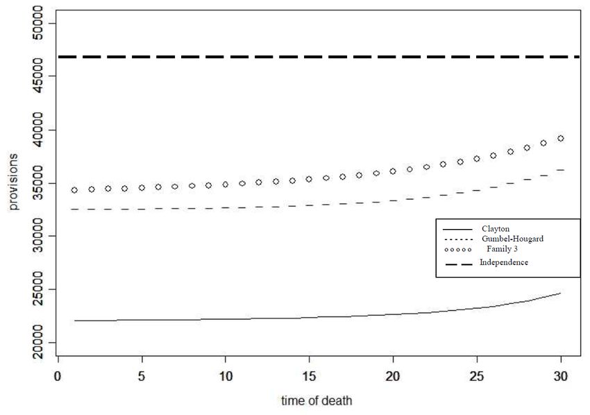
Figure 1: Reserves for time of death of person aged y at period 10.
We assume an insurance contract for a couple of 60 years old. As long as a person
(male regardless of the state of the woman) is alive, the insurer liabilities are 10,000 units
at the beginning of each year. Table 3 provided the percentage of difference in calculated
reserves average using some copulas in Archimedean family (Clayton, Gumbel-Hougaard
and Family 3) relative to the independence copula for the time period of 10, 20, and 30STATISTICS IN TRANSITION new series, March 2021 223
Figure 2: Reserves for time of death of person aged y at period 20.
Figure 3: Reserves for time of death of person aged y at period 30.
years. Moreover, the Kendall’s tau coefficient defined in Eq. (4) is 0.5 at the start point of
the contract with an annual interest rate of 4%. Table 3 demonstrated that applying copula in
Table 3: The percentage of difference in calculated reserves average using Archimedean
copula relative to the independence copula
Copula period 10 period 20 period 30
Clayton -29.2 -36 -44
Gumbel-Hougaard -38.1 -28.7 -15.5
Family 3 -11.5 -11.3 -14
Family 3 reduced the reserve from 11% through 14% compared to the independence copula
in the case that if one of the persons died at the age of y for 10, 20, and 30 years. As can be224 H. Safari-Katesari, S. Zaroudi: Analysing the impact of dependency ...
seen from Figures 1, 2, and 3, the reserves for all three copulas are less than independence
case during the time. Figure 1 shows the reserve at the time period of 10 years which the
copula of Family type 3 has the highest and the Gumbel-Hougaard copula has the lowest
amount of reserve. Figure 2 and Figure 3 displayed the reserves at the time period of 20
years and 30 years, respectively, which the Family 3 has the highest, and the Clayton has
the lowest amount of reserves. To this end, our estimation results indicate that the insurer’s
reserves with using Archimedean copula families are less than the independence case, which
increases the solvency of insurance companies.
5. Conclusion
Since life insurance reserves are calculated by the death of one individual, dependency
of the two lifetimes plays an important role for actuarial computations of insurance compa-
nies. In this paper, the insurer’s reserves are calculated using some Archimedean copulas
for different time periods. The results showed that fitting the appropriate copula optimizes
the amount of insurers’ funds, which can be spent for reserves of future liabilities. Thus,
considering dependency between two lifetimes for calculating the optimal reserves by the
insurer is highly recommended.
References
CARRIERE, J. F., (2000). Bivariate survival models for coupled lives. Scandinavian Actu-
arial Journal, (1), pp. 17–32.
DENUIT, M., DHAENE, J., GOOVAERTS, M., and KAAS, R., (2005). Actuarial theory
for dependent risks: measures, orders and models. John Wiley and Sons.
FREES, E. W., VALDEZ, E. A., (1998). Understanding relationships using copulas. North
American actuarial journal, 2(1), pp. 1–25.
GENEST, C., MACKAY, J., (1986a). The joy of copulas: Bivariate distributions with uni-
form marginals. The American Statistician, 40(4), pp. 280–283.
GENEST, C., MACKAY, R. J., (1986b). Copules archimédiennes et families de lois bidi-
mensionnelles dont les marges sont données. Canadian Journal of Statistics, 14(2),
pp. 145–159.STATISTICS IN TRANSITION new series, March 2021 225
GERBER, H. U., (1997). Life insurance mathematics. Springer Science and Business Me-
dia.
HOUGAARD, P., (2000). Analysis of multivariate survival data. Springer Science and
Business Media.
JI, M., HARDY, M., and LI, J. S. H., (2011). Markovian approaches to joint-life mortality.
North American Actuarial Journal, 15(3), pp. 357–376.
KATESARI, H. S., VAJARGAH, B. F., (2015). Testing Adverse Selection Using Frank
Copula Approach in Iran Insurance Markets. Journal of mathematics and computer
Science. 15(2), pp. 154–158.
KATESARI,H. S., ZARODI, S., (2016). Effects of Coverage Choice by Predictive Model-
ing on Frequency of Accidents. Caspian Journal of Applied Sciences Research, 5(3),
pp. 28–33.
KLUGMAN, S. A., PARSA, R., (1999). Fitting bivariate loss distributions with copulas.
Insurance: mathematics and economics, 24(2), pp. 139–148.
LEE, I., LEE, H. and KIM, H.T., (2014). Analysis of reserves in multiple life insurance
using copula. Communications for Statistical Applications and Methods, 21(1), pp. 23–43.
MARI, D., KOTZ, S., (2004). Correlation and Dependent. Imperial College Press.
NELSEN, R. B., (2006). An Introduction to Copulas. Springer Science and Business Media.
SAFARI-KATESARI, H., ZAROUDI, S., (2020). Count copula regression model using
generalized beta distribution of the second kind. Statistics in Transition New Series,
21(2), pp. 1–12.
SKLAR, M., (1959). Fonctions de repartition an dimensions et leurs marges. Publ. inst.
statist. univ. Paris, 8, pp. 229–231.
SPREEUW, J., (2006). Types of dependence and time-dependent association between two
lifetimes in single parameter copula models. Scandinavian Actuarial Journal, 5, pp.
286–309.
SPREEUW, J., OWADALLY, I., (2013). Investigating the broken-heart effect: a model for
short-term dependence between the remaining lifetimes of joint lives. Annals of Actu-
arial Science, 7(2), pp. 236–257.226 H. Safari-Katesari, S. Zaroudi: Analysing the impact of dependency ... ZAROUDI, S., BEHZADI, M. H., and FARIDROHANI, M. R., (2018a). Application of Copula in Life Insurance. International Journal of Applied Mathematics and StatisticsTM , 57(3), pp. 162–168. ZAROUDI, S., BEHZADI, M. H., and FARIDROHANI, M. R., (2018b). A Copula Ap- proach for Finding the Type of Dependency with Mortality Force Function in Insur- ance Market. Journal of Advances and Applications in Statistics, 53(2), pp. 103–121.
You can also read