Analysis of Driver Knee Contours for Vehicle Interior Design - UMTRI-2018-1 Matthew P. Reed University of Michigan Transportation Research ...
←
→
Page content transcription
If your browser does not render page correctly, please read the page content below
Analysis of Driver Knee Contours for Vehicle Interior Design

                          Matthew P. Reed

       University of Michigan Transportation Research Institute

                            Final Report

                           UMTRI-2018-1

                              April 2018

                                  i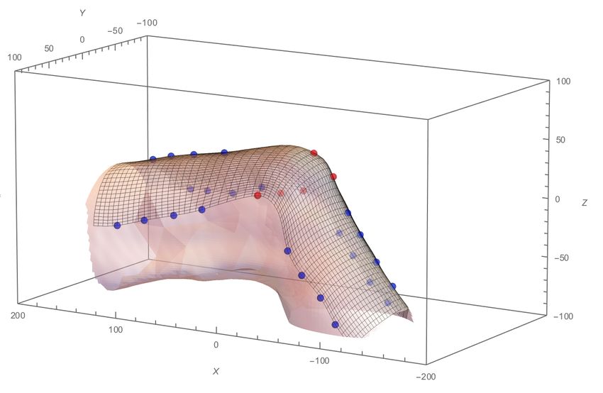
Technical Report Documentation Page
 1. Report No.                                 2. Government Accession No.                         3. Recipient's Catalog No.
 UMTRI-2018-1
Analysis of Driver Knee Contours for Vehicle Interior Design                                      5. Report Date

                                                                                                  6. Performing Organization Code

7. Author(s)                                                                                      8. Performing Organization Report No.
Reed, M.P.
9. Performing Organization Name and Address                                                       10. Work Unit No. (TRAIS)
University of Michigan Transportation Research Institute
2901 Baxter Rd.                                                                                   11. Contract or Grant No.
Ann Arbor MI 48109
12. Sponsoring Agency Name and Address                                                            13. Type of Report and Period Covered
General Motors
                                                                                                  14. Sponsoring Agency Code

15. Supplementary Notes

16. Abstract
An analysis of knee contours was conducted to provide design guidelines to prevent inadvertent actuation of switches
located in the lower part of the driver compartment. A programmatic analysis of 3D laser scan data from 181 men and
women was conducted. The results quantified the maximum level of penetration into a circular opening that could be
expected. The maximum penetration was generally observed in the lateral patella area. A statistical model of the data
was used to generate plots of the distributions of penetrations that would be observed for circular holes of various size.
A verification study was conducted using manual measurements on a convenience sample of 42 people. The results of
the manual measurements were generally consistent with the programmatic measurements from 3D scans, with
discrepancies typically less than 3 mm for holes up to 50 mm.

17. Key Words                                                                 18. Distribution Statement
Crash safety, vehicle maneuvers, occupant motions

 19. Security Classif. (of this report)             20. Security Classif. (of this page)                   21. No. of Pages     22. Price
                                                                                                                      21

Form DOT F 1700.7 (8-72)                  Reproduction of completed page authorized

                                                                          i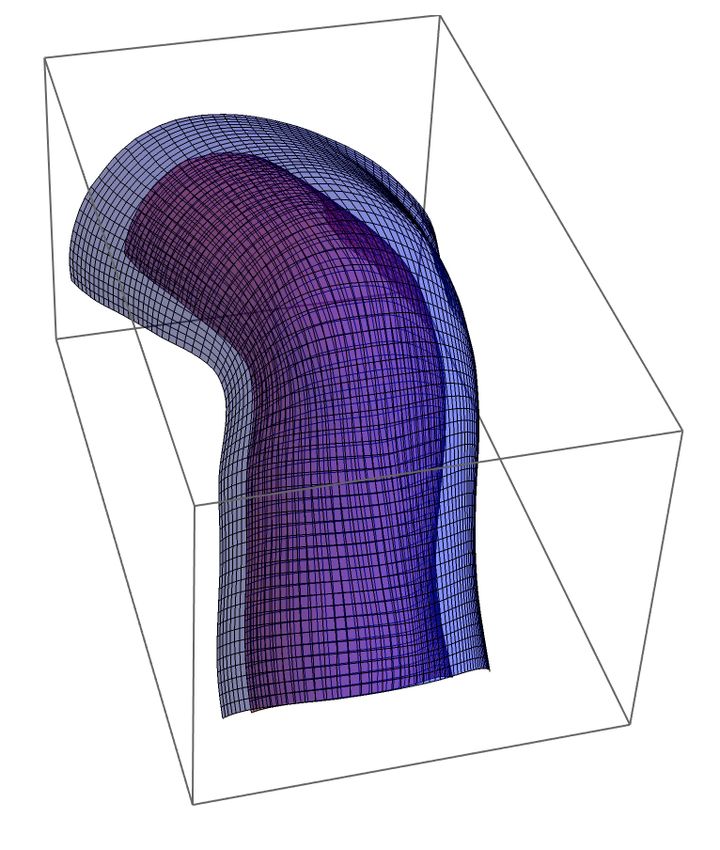
Metric Conversion Chart
                                APPROXIMATE CONVERSIONS TO SI UNITS
SYMBOL                       WHEN YOU KNOW    MULTIPLY        TO FIND                                   SYMBOL
                                                BY
                                                       LENGTH
    In                inches                            25.4                millimeters                 mm
    Ft                feet                              0.305               meters                      m
   Yd                 yards                             0.914               meters                      m
   Mi                 miles                             1.61                kilometers                  km
                                                         AREA
         2
    in                squareinches      645.2                  square millimeters                       mm2
    ft2               squarefeet        0.093                  square meters                            m2
   yd2                square yard       0.836                  square meters                            m2
    Ac                acres             0.405                  hectares                                 ha
   mi2                square miles      2.59                   square kilometers                        km2
                                                       VOLUME
              fl oz                  fluid 29.57                   milliliters             mL
                                     ounces
                 gal                 gallons 3.785                 liters                  L
                     3
                 ft                  cubic    0.028                cubic meters            m3
                                     feet
              yd3                    cubic    0.765                cubic meters            m3
                                     yards
NOTE: volumes greater than 1000 L shall be shown in m3
                                                         MASS
              oz                   ounces      28.35                          grams         g
              lb                   pounds      0.454                          kilograms     kg
                 T                 short       0.907                          megagrams Mg (or "t")
                                   tons                                       (or "metric
                                   (2000                                      ton")
                                   lb)
                                           TEMPERATURE (exact degrees)
             o                                                                                  o
                 F               Fahrenheit            5 (F-32)/9            Celsius                C
                                                       or (F-32)/1.8
                                        FORCE and PRESSURE or STRESS
             lbf                poundforce 4.45                                           newtons       N

                                                                                                              2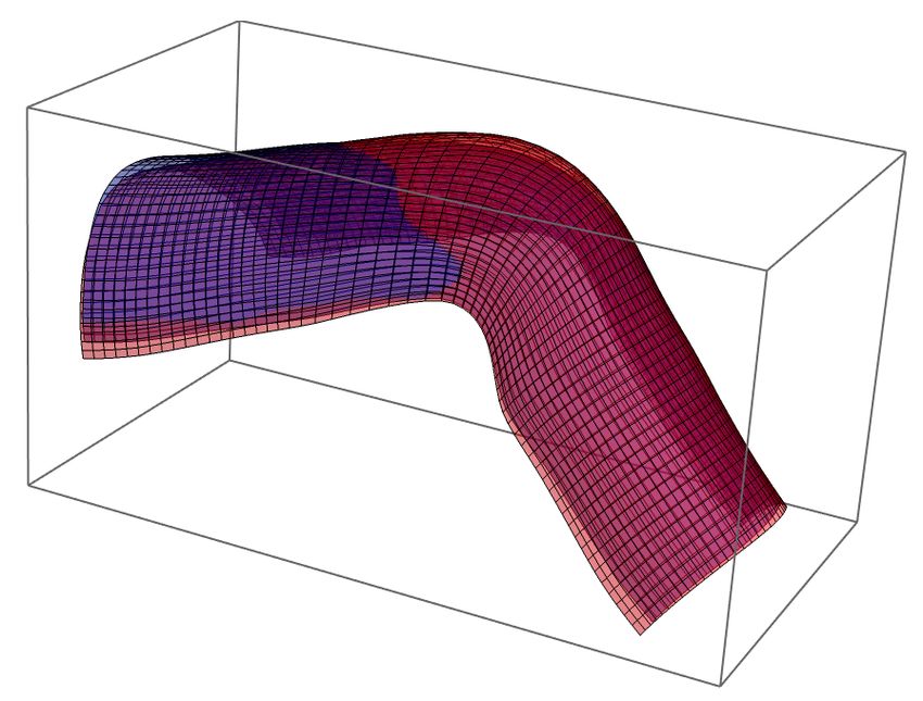
lbf/in2                   poundforce 6.89                            kilopascals kPa
                                per square
                                inch
                                                      LENGTH
         mm                    millimeters           0.039               inches in
             m                 meters                3.28                feet       ft
             m                 meters                1.09                yards yd
         km                    kilometers            0.621               miles mi
                                                       AREA
                 2
      mm                  square             0.0016                     square       in2
                          millimeters                                   inches
         m2               square meters      10.764                     square       ft2
                                                                        feet
         m2               square meters      1.195                      square       yd2
                                                                        yards
         ha               hectares           2.47                       acres        ac
              2
      km                  square             0.386                      square       mi2
                          kilometers                                    miles
                                                      VOLUME
    mL                milliliters                   0.034        fluid ounces            fl oz
     L                liters                        0.264        gallons                 gal
         3
     m                cubic meters                  35.314       cubic feet              ft3
     m3               cubic meters                  1.307        cubic yards             yd3
                                                       MASS
         g               grams                0.035                    ounces              oz
      kg                 kilograms            2.202                    pounds              lb
  Mg (or "t")            megagrams (or        1.103                    short tons          T
                         "metric ton")                                 (2000 lb)
                                         TEMPERATURE (exact degrees)
     o                                                                                         o
         C             Celsius                    1.8C+32         Fahrenheit                       F
                                        FORCE and PRESSURE or STRESS
     N               Newtons                   0.225               poundforce                      lbf
    kPa              Kilopascals               0.145               poundforce per lbf/in2
                                                                   square inch

*SI is the symbol for the International System of Units. Appropriate rounding should
be made to comply with Section 4 of ASTM E380.
(Revised March 2003)

                                                                                                         3
ACKNOWLEDGMENTS

This research was supported General Motors LLC. The body scan data used for the
retrospective analysis were gathered with support from the Toyota Collaborative Safety
Research Center. Sheila Ebert of UMTRI coordinated all data collection and assisted with
the scan data extraction.

                                                                                       4
CONTENTS

ACKNOWLEDGMENTS.................................................................................................

ABSTRACT .....................................................................................................................

INTRODUCTION ............................................................................................................

METHODS.......................................................................................................................

RESULTS ........................................................................................................................

DISCUSSION...................................................................................................................

                                                                                                                               5
ABSTRACT

An analysis of knee contours was conducted to provide design guidelines to prevent
inadvertent actuation of switches located in the lower part of the driver compartment. A
programmatic analysis of 3D laser scan data from 181 men and women was conducted.
The results quantified the maximum level of penetration into a circular opening that
could be expected. The maximum penetration was generally observed in the lateral
patella area. A statistical model of the data was used to generate plots of the distributions
of penetrations that would be observed for circular holes of various size. A verification
study was conducted using manual measurements on a convenience sample of 42 people.
The results of the manual measurements were generally consistent with the programmatic
measurements from 3D scans, with discrepancies typically less than 3 mm for holes up to
50 mm.

                                                                                            6
INTRODUCTION

The design and placement of switches in vehicle interiors must include consideration of
the potential for inadvertent activation. For switches located in the lower part of the
driver area, contact with the driver’s knee is a possibility. The current project considered
the situation of push-button switch recessed within a circular opening. The goal of the
research was to estimate the depth of switch placement that would be sufficient to greatly
reduce or eliminate the possibility of activation by a driver’s knee. The research was
conducted in two phases. First, a large set of three-dimensional (3D) body surface scan
data was queried to estimate the maximum penetration possible with a range of hole
sizes. Second, hole penetrations were manually measured for a convenience sample of
knees to verify the findings from the 3D scan study.

METHODS –– SCAN-BASED MEASUREMENTS

Surface scan data for right knees were extracted from scan data obtained in a large study
of driver postures and body shapes. Figure 1 shows the two postures from which the data
were extracted. The included knee angle was either 90 or 115 degrees (approximately
typical driving posture). Knees were extracted from scans of 181 men and women in the
automotive posture and 83 in the 90-degree posture.

                 Figure 1. Scan poses used: automotive (left) and 90-degree (right).

For each extracted scan, the locations of four landmarks were available: medial femoral
condyle (MFC), lateral femoral condyle (LFC), suprapatella, and infrapatella. These
landmark locations are shown in Figure 2. To facilitate programmatic analysis, a
rectangular grid was fit to the anterior surface of each scan, using the landmarks to ensure
that the grid placement was homologous for each knee.

Figure 2 shows the grid mesh, which was composed of 3111 vertices and is homologous
to a half cylinder. In addition to the LFC and MFC landmarks, 12 synthetic landmarks

                                                                                           7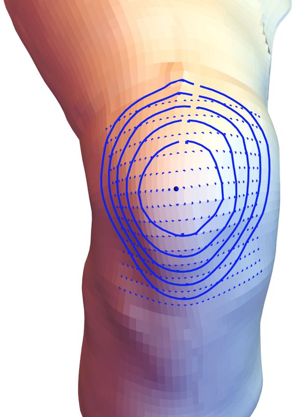
were generated on the thigh and 12 on the leg to guide the fitting. The suprapatellar
landmark was also used to ensure its position would be homologous across fitted scans.

Figure 2. Example of quadrangle mesh (black lines) fit to knee scan. Digitized landmarks are shown
in red. Synthetic landmarks used to align the mesh are shown in blue.

Statistical analysis was conducted on the fitted mesh data from the automotive posture.
Sex, stature, body mass index (BMI), and sitting height (expressed as the ratio of sitting
height to stature, SHS) were included as predictors. Interestingly, stature has very little
effect on knee size and shape, holding other variables constant (Figure 3). Sex also has a
minimal influence on knee shape (Figure 4). BMI has the largest effect; individuals with
high BMI have on average much wider knees (Figure 5).

                                                                                                     8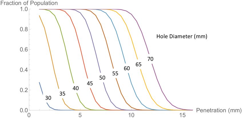
Figure 3. Small female (blue) and large male (red) predicted knee shape holding BMI=27.5 and
SHS=0.52. Statures are 1511 and 1870 mm, respectively.

                 Figure 4. Male (red) vs. female (blue) after accounting for stature,
                                      BMI, and sitting height.

                                                                                               9
Figure 5. Mid-stature male with BMI=20 (red) and BMI=35 kg/m2 (blue).
Simulating Hole Penetration – Automotive Posture
A simulation method was developed to determine how far each knee could penetrate into
holes of various sizes. The method is illustrated schematically in Figure 6. For each mesh
point in an area near the patella, planar slices were taken along the normal vector at 5-
mm increments into the knee. The maximum distance across the slice was determined.
This is effectively the diameter of the smallest circular hole into which the knee could
penetrate to the specified depth centered on the selected vertex. Repeating this across the
knee and taking the smallest slice width for each depth (5, 10, 15, 20, & 25 mm) gives,
for each knee, the minimum hole size the knee can penetrate each distance.
10Figure 6. Estimating penetration at 5, 10, 15, 20, and 25-mm increments along the normal for one
sample point on the knee (large dot). All sample points are shown with small blue dots.
Figure 7 shows the results from automotive posture scans. The cumulative distributions
of across 181 subjects are plotted. The distributions are approximately log-normal. The
interpretation of the curves is as follows, for example: approximately a 65-mm-diameter
hole is needed to allow 50% of the knees to penetrate at least 10 mm. For that same 65-
mm-diameter hole, essentially all knees would be able to penetrate 5 mm, but almost
none would penetrate 15 mm or more.
Figure 7. Distributions of the minimum widths for penetrations of 5, 10, 15, 20, and 25-mm (left to
right) for 181 men and women.
The areas of greatest penetration (effectively the “pointiest” area of the knee) lay on the
outside of the patella area. Figure 8 shows the locations of these sample points on an
11exemplar knee. This participant had the smallest max section widths at 10, 15, and 20
mm, effectively showing the highest penetrations (Figure 9).
Figure 8. Locations of 10 sample points with the highest penetrations across subjects (smallest
diameters at each penetration level) on an exemplar knee. (These are not necessarily the points of
highest penetration on this knee.) The lateral aspect is at the bottom of the figure.
Figure 9. “Pointiest knee”, demonstrating the greatest penetrations (subject T098, male, 1699 mm tall,
80 years old, BMI 30.4 kg/m2).
The most useful predictor of knee penetration depth is body mass index (BMI).
Figure 10 shows the minimum hole width for 10 mm penetration as a function of BMI.
12This is consistent with the earlier finding that lower BMI is associated with narrower
knees, but small stature is not. A consequence of this finding is that further investigation
of knee penetrations should focus on low BMI populations, regardless of stature, gender,
or age.
Figure 10. Hole width for 10-mm penetration (smaller indicates greater pointiness) as a function of
BMI (kg/m2). The pointiest-knee subject from Figure 9 is seen here as a low outlier at BMI 30.4.
Simulating Hole Penetration – 90-Degree Posture
The same method used previously was implemented to measure hole penetration with the
90-degree scans. Figure 11 shows the contours on the sample planes for sample point on
one knee.
As with the automotive-posture data, the largest width of the plane contour was obtained
for each sample point, corresponding to the minimum diameter hole that the knee could
penetrate to the prescribed depth at that point. For each penetration depth, the smallest
value across the knee was extracted; this corresponds to the smallest hole into which that
subject’s knee could penetrate by the prescribed amount.
Figure 12 shows these results per sample plane across 83 subjects and provides a
comparison with the values obtained using the automotive-like knee flexion (included
angle about 115˚). The differences for small amounts of penetration are not large. For
example, the median width for 5 mm of penetration is around 45 mm in both postures.
Larger differences are observed for greater penetration levels, but at the median the
differences are still typically less than 5 mm. The lack of posture effects for small
penetrations is because these penetrations are influenced predominantly by the local
shape around the patella, which is not strongly affected by knee angle.
13Figure 11. Estimating penetration at 5, 10, 15, 20, and 25-mm increments along the normal for one
sample point on the knee (large dot). All sample points are shown with small blue dots.
Figure 12. Distributions of the minimum widths for penetrations of 5, 10, 15, 20, and 25-mm (left to
right) for 83 men and women with 90-degree included knee angle (dashed lines) and 181 men and
women with 115-degree included knee angle (solid lines). Example Interpretation: only about 10% of
knees can penetrate more than 10 mm into a 60-mm-diameter hole
As with the previous analysis, the areas of greatest penetration (effectively the pointiest
points) lay on the outside of the patella area. One participant had the smallest max section
widths at all depths, effectively showing the highest penetrations. This “pointiest knee” is
shown in Figure 13. As before, the most useful predictor of knee pointiness (penetration)
14is body mass index (BMI). Age and overall body size (stature) had much weaker
relationships.
Figure 13. “Pointiest knee” in 90-deg scans, demonstrating the greatest penetrations. (subject T098,
male, 1699 mm tall, 80 years old, BMI 30.4 kg/m2)
The cumulative distributions of hole width for each penetration depth are approximately
log-normal. Figure 14 shows log-normal approximations for each penetration depth.
Using these distributions, the functions can be inverted to be more useful for analysis.
Figure 15 shows the population distribution of penetrations for a range of hole diameters,
based on the log-normal fits in Figure 14. The plot shows the distribution of maximum
penetrations given the specified hole diameter. For example, consider a penetration of 10
mm. From Figure 15, we expect that nearly all people to require a whole size larger than
50 mm to achieve 10 mm of penetration. In Figure 12, the fraction of the population
achieving 10 mm of penetration with a 50-mm hole is close to zero.
15Figure 14. Cumulative log-normal distribution approximations (solid lines) for empirical distributions
of hole diameter across penetration depths from Figure 12.
Figure 15. Distribution of penetration depths for a range of hole diameters based on log-normal
approximation.
16RESULTS – VERIFICATION STUDY
The scan-based analysis provided inexpensive analysis to a large dataset, but the
scanning and data processing steps may have tended to smooth the surface, resulting in
smaller penetration estimates. Moreover, any effect of soft-tissue deformation would not
be captured by the scan-based analysis. Consequently, a small verification study was
conducted to compare manual measurements with the scan-based results.
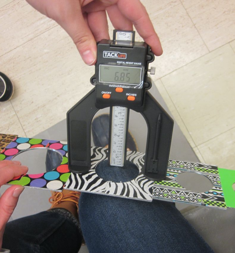
A series of holes were cut in a sheet of 2.25-mm-thick aluminum. As shown in Figure 16,
the hole fixture was manipulated to obtain the greatest penetration at each hole diameter
from 30 to 70 mm. The penetration was measured to 0.1 mm using a manual depth gage.
The fixture thickness was added to each measurement. Data were gathered from a
convenience sample of 42 young men and women with a wide range of body size.
Figure 18 shows an overview of the participants’ characteristics. Data were gathered with
people wearing their normal clothing, which included jeans, tights, and no clothing over
the knee.
Figure 16. Measuring penetration.
17Figure 17. Anthropometric data for N=42 participants in verification study.
18Figure 18 shows a boxplot of the data across hole diameter. The distributions within each
hole size are approximately symmetrical and the median penetration is an approximately
linear function of hole diameter. As in the previous analysis, slightly smaller penetrations
were observed for individuals with higher BMI (Figure 19).
Figure 18. Boxplot of measured penetration for a range of hole diameters (N=42 for each diameter).
Figure 19. Effects of BMI on penetration depth in verification dataset.
19The distributions of penetration depths can be compared to the estimates from obtained
from the scan-based analysis. Figure 20 shows cumulative plots of the manual data
(inverted to show fraction exceeding the penetration depth on the horizontal axis).
Predictions from the scan-based model (90-deg posture) are also shown. The manual-
measurement data show greater penetration than the scan-based model for all hole
diameters, but the differences are small in absolute terms. For example, the prediction
model shows essentially zero penetrations more than 10 mm for a 40-mm-dimeter hole.
The maximum value in the verification data was about 12 mm.
Figure 20. Comparison of verification data (dashed lines) with predictions from scan data (solid lines).
The vertical axis is cumulative population fraction exceeding the penetration depth on the horizontal
axis for range of hole diameters.
20DISCUSSION
The scan-based analysis was largely verified by the manually measured sample. Both
methods have some limitations that should be considered. The knees were scanned nude,
but as noted above the scanning and analysis process may have smoothed the surface
somewhat and flesh deformation is not taken into account. Moreover, the penetration
simulation method was based on the local normal. In some circumstances, greater
penetration could be obtained using a surface that is not orthogonal to the normal at the
center of the simulated hole. The manually measured sample included a range of normal
clothing; 16 of the 42 participants wore jeans and 8 had nude knees. Greater penetrations
might have been measured if all participants were measured directly on the skin.
Although a weak effect of BMI was observed, no attempt was made to normalize the
results to a particular population BMI distribution. The effort is not warranted given that
the adjustment is small relative to uncertainties in the BMI distribution.
The parametric models generated in this work can be used to estimate tail percentiles of
the penetration distributions. An alternative approach would be to manually measure
penetrations for a larger sample of people, specifically targeting those with low BMI,
including the youngest and oldest drivers, who are more likely to have lean knees.
The current work does not consider some foreseeable situations, such as individuals with
prosthetics or braces on their knees. Further study would be needed to identify the
penetrations that could be associated with such devices.
21You can also read