Antifragility of Real Estate Investments in a World of Fat-Tailed Risk

Antifragility of Real Estate Investments in a
 World of Fat-Tailed Risk*

 Authored by

 Guy Tcheau, Managing Director, Principal Real Estate Investors

 Norman Miller, PhD, Ernest Hahn Chair and Professor of Real Estate
 Finance, University of San Diego School of Business and affiliated with the
 Burnham-Moores Center for Real Estate
 *

*Disclaimer: All errors are ours. The views expressed herein are solely those of the authors and
 do not necessarily represent the views of Principal Real Estate Investors or the University of
 San Diego School of Business or the Burnham-Moores Center for Real Estate.

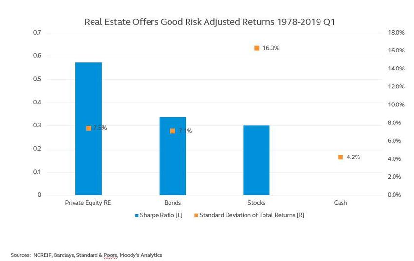
Antifragility of Real Estate Investments in a World of Fat-Tailed Risk*
 † Guy Tcheau
 ‡ Norman Miller, PhD

Abstract

Investors have sought to add real estate to their multi-asset portfolios due to the
lower volatility, higher component of total return from income, diversification and
tangible nature associated with real estate relative to other assets generally. Real
estate is often seen as defensive in this regard. Exogenous shocks or Black Swan
events, such as Covid-19, are by definition, ‘unknowable’ with respect to
occurrence and consequence and therefore susceptible to the limitations of
statistical models, a priori. This paper examines real estate investing, not just from
whether it is defensive, but whether it has antifragility characteristics. Antifragility
refers to an investment that is not only robust to exogenous shocks but benefits
from such shocks. We show from first principles and from empirical data that real
estate has antifragility and warrants higher allocations to multi-asset portfolios for
this reason.

Introduction

 1.1 Real Estate investments provide several key benefits when added to a
 multi-asset portfolio. These benefits stem from real estate’s inherently
 low volatility and low correlation vis-a-vis asset classes such as stocks
 and bonds, as well as inflation hedging potential1. In the traditional
 Markowitz modern portfolio theory construct, real estate improves the risk
 / return profile by enhancing the mean-variance efficient frontier in a
 multi-asset portfolio2. The diversification benefits from private real estate
 benefit portfolios in both down and up markets3. The high proportion of
 total return attributable to current income versus appreciation coupled
 with contractual leases from tenants that undergird the income yield adds
 defensiveness to the overall portfolio.

 1.2 One might argue that real estate returns, risk adjusted, i.e. for volatility,
 have proven superior to stocks and bonds. The chart below shows real
 estate having the highest Sharpe Ratio vis-à-vis the other asset classes.
 The Sharpe Ratio is aimed at measuring how well a portfolio’s return
 compensates the investor for risk. It is the excess return of an investment
 portfolio over the risk-free rate divided by standard deviation of the

 1

returns. Higher returns are not necessarily superior, if it is accompanied
 by higher variability in the returns. It is the returns per unit of risk that the
 Sharpe Ratio measures. The higher the Sharpe Ratio the better the
 returns relative to risk, measured in this fashion.

*Disclaimer: All errors are ours. The views expressed herein are solely those of the authors and
 do not necessarily represent the views of Principal Real Estate Investors or the University of
 San Diego School of Business or the Burnham-Moores Center for Real Estate.

† Guy Tcheau, Managing Director, Principal Real Estate Investors
‡ Norman Miller, PhD | Ernest Hahn Chair and Professor of Real Estate Finance, Burnham-Moore
Center for real Estate, University of San Diego School of Business

 2

1.3 In addition, real estate investments can be accessed via four quadrants
 which provides a menu of risk and return alternatives for the investor.
 EQUITY VS DEBT
 INCOME & APPRECIATION YIELD & DOWNSIDE PROTECTION

 PRIVATE DEBT :
 PUBLIC VS PRIVATE

 PRIVATE EQUITY :
 LONGER EXECUTION & LOWER Senior mortages, Mezzanine loans
 Core, Value-Add
 VOLATILITY Construction loans
 Opportunistic
 Participating loans

 PUBLIC EQUITY : PUBLIC DEBT :
 LIQUIDITY & HIGHER Listed developers AAA - Non-investment grade CMBS
 VOLATILITY Public REITs Interest only CMBS
 Preferred Securities REIT unsecured debt

 These four quadrants are obtained by combinations along two
 dimensions, namely public vs private and equity vs debt as shown in the
 figure above.

1.4 This paper examines the attractiveness of real estate investing from
 another vantage point called ‘robustness and anti-fragility’. This thesis
 flows primarily from the published work of Nassim Taleb on the subject
 of mathematical finance, uncertainty and randomness. By coincidence,
 the fourth quadrant is also referred to by Taleb in his book the Black
 Swan. However, the two dimensions in Taleb’s model are simple payoffs
 vs complex payoffs and thin-tailed vs fat-tailed distributions of outcomes.
 The fourth quadrant thus refers to financial outcomes that cannot be
 modeled or statistically quantified with sufficient robustness to permit
 qualified decision making. This quadrant is the domain of Black Swans,
 where investors are susceptible to the limitations of statistical models as
 applied to real world finance because of what Taleb calls the ‘unknown
 unknowns’4.

1.5 Institutional investors such as pension plans typically have an allocation
 of their multi-asset portfolios to real estate. Prior to the current Covid-19
 dislocation, real estate allocations for pension plans were averaging
 about 10.4% versus target allocations of 11.4% based on surveys by
 leading real estate associations (PREA, INREV and ANREV)10. Due to the
 decline in the stock market, these real estate allocations are likely to be
 near or overweight the targets due to the denominator effect, i.e., the fall
 3

in value of the overall portfolio relative to real estate value adjustments.
 Given the antifragile nature of real estate it can be argued that target
 allocations to real estate ought to be increased.

2. Probability Distribution

 2.1 Let us examine the two ways to view the real world; the first of which
 Taleb calls ‘mediocristan’5. In this view, outcomes are fairly predictable
 and stable. Within a large sample size, no single outlier outcome
 significantly impacts the aggregate total. Mediocristan is characterized
 by event probability distributions that tends towards the traditional thin-
 tailed normalized distribution. In other words, there exists a mild
 randomness which is reasonably easy to parametrize and model.

 2.2 The other view of the world, which is rarely used in finance, is called
 ‘extremistan’5. Here, one outlier observation can materially distort the
 aggregate. Randomness is not mild but severe. Rather than a
 normalized bell-shaped probability distribution we have instead a fat or
 fat-tailed curve. Outcome distributions are skewed or have high
 kurtosis6.

 2.3 It follows that that given the two sets of outcomes i.e. mediocristan or
 extremistan, we will have two distinct categories of investment decisions
 depending on whether mild or severe randomness is in force.
 Mediocristan based decisions are generally simple and binary i.e. either
 yes or no; true or false. Decisions are based solely on probability of
 events and are not impacted by the consequence of the outcome.
 Extremistan based decisions are much more involved. Both the
 probability of an event and the consequence of the outcome have to be
 considered in tandem.

 4

SIMPLE PAYOFF COMPLEX PAYOFF

 EVENT PROBABILITY THIN TAILED, NORMAL High Certainty & Low Consequence High certainty & Large Consequence
 DISTRIBUTION OF EVENT Highly Predictable Outcomes Somewhat Predictable Outcomes
 FREQUENCY Robust to Black Swans Fairly robust to Black Swans

 THICK TAILED OR Less Certainty & Low Consequence Less Certainty & Large Consequence
 ASSYMETRIC DISTRIBUTION Somewhat Predictable Outcome Unpredictable Potentially Big Outcomes
 OF EVENT FREQUENCY Fairly Robust to Black Swans Extreme Fragility to Black Swans

 4th Quadrant
2.4 Traditional financial models based on mean variance assumes
 normalized Gaussian distributions and thin tails6&7. The normalized
 distribution clusters outcomes symmetrically around the mean where the
 probability of an outcome being 2 standard deviations away from the
 mean is under 5%. The probability falls to 0.3% if the outcome is 3
 standard deviations away from the mean. Thin tails refer to very low
 probability of outcomes occurring outside of 3 standard deviations or
 three-sigma from the mean. However, the reality is that the measures of
 averages and variances that are relied on can be very misleading
 because distributions in the real world are more asymmetric than
 commonly assumed. Furthermore, so called thin tailed outliers occur with
 higher frequency then implied by normalized distributions. We call
 probability distributions fat tailed when the outcomes that deviate from
 the mean by 3 or more standard deviations are materially higher than
 implied in a normalized distribution.

2.5 As a consequence, portfolio construction based on mean variance
 modeling, while generally effective in 3 of the 4 outcome scenarios,
 become fraught with risks when applied to the 4th quadrant due to the
 high degree of fragility to Black Swan events. A casual observation of the
 Global Financial Crisis, Covid-19 and other systemic shocks bears
 witness to the impact of outcomes in the 4 th quadrant.

2.6 With the benefit of hindsight, financial market participants adjust
 quantitative models to account for the latest systemic shock followed up
 by stress tests to derive comfort that portfolios will be immunized from
 repeat debacles. However, the problem with ‘unknown unknowns’ is that

 5

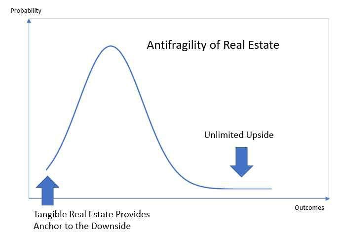
it falls outside the bounds of robust statistics and quantitative models,
 prima facie.

3. Antifragility

 3.1 There are essentially four outcomes as shown below 8. Robust outcomes
 are where outlier events have low probability and have small
 consequence, either positive or negative. Investment performances are
 fairly predictable since outcomes are not materially impacted by shocks.
 However, there are two types of fragile outcomes: symmetric and
 asymmetric, which are both descriptors of downside scenarios. Both give
 rise to more negative impacts since the tails are fat. Asymmetric tails to
 the left means that the investment is more fragile to negative outcomes
 than to positive upsides. Antifragile9 investments, on the other hand, are
 asymmetric to the right. Here the fat tail to the upside means outliers
 tend to be positive with large payoffs. In short, robust investments are
 agnostic to volatility whereas antifragile investments benefit from
 dislocations. Fragility implies that investments tend to go very badly with
 volatility.

 3.2 What exactly are antifragile investments? These are investments that
 benefit from volatility. Mathematically this is referred to as convexity.

 6

Convexity under Taleb’s model is different from convexity that is used for
 bond investments. For bonds, convexity measures the change in the
 price of the bond in relation to changes in the level of interest rates. As
 the diagram below illustrates, the higher the volatility in the events under
 Taleb’s model the greater the payoff with convexity12. Conversely,
 greater volatility results in greater losses for concavity.

 3.3 With these 4 outcomes in mind, Taleb advocates the majority of a
 portfolio be concentrated in robust investments with a small portion in
 antifragile investments. Fragile investments are to be shunned
 altogether. This barbell strategy seeks to resolve the problem with
 extremistan and the 4th quadrant of Black Swan event.

4. Antifragility of Private Equity Real Estate

 7

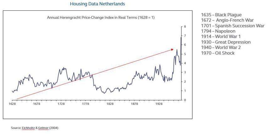
4.1 We believe that private equity real estate exhibits antifragile
 characteristics because of its asymmetric return profile that is skewed
 right. While these antifragile characteristics may have some degree of
 manifestation in real estate debt or publicly traded REITs, it is most
 pronounced and observable in private equity real estate performance.
 We focus on the private equity real estate exclusively when examining
 antifragility and convexity.

4.2 With public equities or corporate bonds for example, in Black Swan
 events, the value of certain securities might tend towards zero. The
 reason is that the underlying businesses can become unviable due to
 shocks. Take for example Lehman Brothers or Bear Stearns during the
 Global Financial Crisis. These firms were no longer able to be remain
 operational. With Covid-19 it remains to be seen whether certain cruise
 ship operators will remain in business, for example. However, with real
 estate there is real tangible property that underpins the investment. Real
 property has been a repository of value for many millennia. Real estate
 provides a non-trivial anchor to the downside which is largely overlooked
 in traditional financial models. Whereas the upside is technically
 unlimited, the downside has a floor. This makes the return distribution
 asymmetric to the right.
4.3 The empirical data on real estate price changes in real terms over very
 long time period of nearly 400 years (See the case study on housing
 prices in Netherlands below) supports asymmetry to the upside and finite
 downside. Despite major Black Swan events such as the Black Plague,
 Napoleanic Wars, both World Wars and the Great Depression, real
 estate showed resiliency to the downside (floors provided by tangible real
 property value) plus fat-tailed upside. Note also, that this period included

 8

the Spanish Flu of 1918 which reportedly infected over 500 million people
 with a death toll between 40 million to 100 million.

4.4 The next question is whether real estate exhibits convexity. On a relative
 return basis, as compared to public traded stocks or corporate bonds,
 real estate fares relatively well during periods of systemic distress.
 Therefore, we can infer that convexity exists in the relative sense. Yet, it
 is true nonetheless, that in the short term, Black Swan events do hurt real
 estate values. Therefore, real estate appears to exhibit concavity in the
 short term. However, when viewed over a longer-term horizon, rather
 than focusing on spot prices, we see evidence that real estate losses halt
 due to its intrinsic real value and then, not just recover, but move to the
 upside.

4.5 The reason is that real estate values are a function of rents paid by
 property occupiers. Rental rates are derived from supply and demand
 forces for both occupiers and suppliers of real estate. Following Black
 Swan events, the supply of capital for construction of new properties
 becomes highly curtailed. This chokes off new supply. However, the
 demand for real estate which is a derivative of population and
 employment increases in aggregate over the long term. This natural
 phenomena for demand results in a rightward shift in the demand curve
 while the supply curve either shifts left (obsolescence) or remains
 relatively constant in the aftermath of shocks. The combined effect leads
 to equilibrium pricing (rents) moving upwards. As rents rise so will real
 estate values, which discounts the stream of rental payments over the

 9

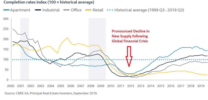
investment horizon. We posit that these forces result in convexity for real
 estate investors.

5. Convexity of Real Estate from First Principles
 5.1 To see the causal effects for convexity we compare the dynamics of real
 estate demand and supply with that of traditional businesses that
 underpin public equities and bonds. In the case of businesses in general,
 the demand side of the supply and demand equilibrium has the larger
 impact on success and viability. Businesses cater to their customers but
 cannot control the state of the customers and their demand at any point
 in time. We characterize businesses in the aggregate as predominantly
 ‘exogenous’.
 5.2 Real estate also caters to their customers who in this instance are the
 property occupiers. Demand is a function of the number of occupiers
 which in turn is a derivative of general population. As noted earlier,
 general population in aggregate increases over the long run. Therefore,
 it follows that occupier demand for real estate has a natural rightward
 shift; that is after smoothing out shorter term cyclical impacts of
 macroeconomic dislocations or localized sociopolitical perturbations. The
 more potent force in the demand supply equilibrium of real estate is the
 supply side. In other words, boom bust cycles in real estate are driven
 more by overbuilding of real estate than by demand side shifts; ceteris
 paribus.
 5.3 We are, of course, speaking about real estate in aggregate as segments
 of real estate by type or geography certainly do react to demand forces.
 Retail for example is greatly impacted by e-commerce, which in turn has
 decimated many bricks and mortar retailers, who are the occupiers of
 retail malls. The destruction of the demand base for retail has materially
 impacted retail mall rents and hence values, while benefitting logistics
 and industrial properties. However, across real estate in aggregate which
 also includes multifamily apartments, office, industrial, hospitality,
 housing, farmland, etc., we can see that demand exhibits less variability
 with a gradual right shift due to population increase. It follows then that
 supply is the principal driver of equilibrium in real estate demand and
 supply interaction. We characterize real estate as predominantly
 ‘endogenous’.
 5.4 Following the Global Financial Crisis, we can see a dramatic drop off in
 the level of new supply across real estate. This stems from fear and risk-

 10

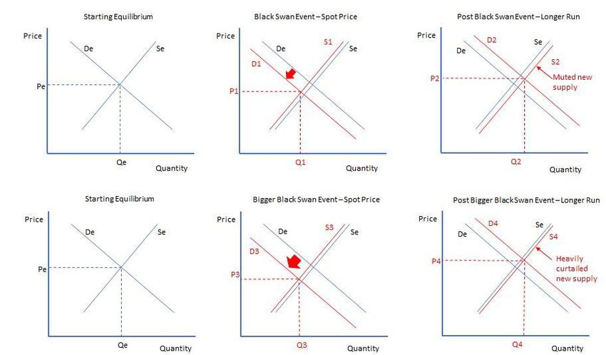
off mentality coupled with anti-risk-taking measures imposed by policy
 makers which act to curtail real estate developers’ access to capital.
 Paradoxically the more severe the shock i.e. greater volatility, the more
 severe the resulting curtailment of new supply. This is precisely the
 necessary force needed in a predominantly endogenously driven
 demand and supply market dynamic to produce the upwards pricing
 equilibria in response to volatility.

5.5 We examine the demand supply equilibria for real estate in the short and
 long run under conditions of increasing volatility (Black Swans) and
 decreasing volatility (strong macroeconomy). Starting with equilibrium
 between demand and supply with Price = Pe and Quantity = Qe we first
 examine the impact of a Black Swan even on the spot price. We see that
 demand falls off materially to D1 due to the shock to aggregate demand.
 There is a drop off in Supply to S1 which is small relative to the fall in
 demand. In real estate, supply decreases due to obsolescence or the
 withdrawal of marginal properties from the market. However, unlike
 manufacturing where production lines can be halted, real estate supply
 is sticky as it is essentially a fixed asset. At the new spot equilibrium,
 price falls to P1P1 and P2>Pe.

 11

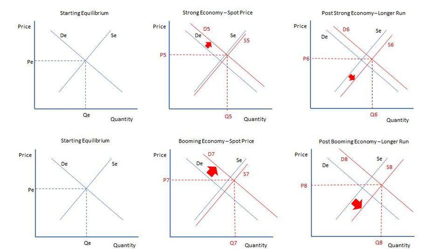
5.6 Paradoxically, the more severe the Black Swan event the stronger the
 curtailment of new supply in the longer run. In a bigger Black Swan
 dislocation, demand falls more dramatically to D3 and price to P3P2, meaning the long run equilibrium achieves higher pricing
 the more severe the Black Swan event.

5.7 Now, let us examine demand and supply equilibria of real estate under
 conditions of economic growth. Here, we have no outlier events and
 volatility of events is declining. In the short run, aggregate demand
 increases to D5 and supply increases to S5. Since new supply in real
 estate is sticky in the short run D5 outweighs S5 and the equilibrium price
 moves to P5>Pe. Since property development requires time to source
 capital, obtain government approvals, mobilize and construct there is a
 lag to new supply. The impact of exuberant macroeconomic conditions
 leads to ample supply of capital for property development. This results in
 a spike in new supply S6 which acts to swamp the growth in demand to
 D6. As noted earlier, real estate equilibrium is predominantly a function

 12

of endogenous forces. We find P6Pe in the short run.
 Interestingly, in the longer run, risk-on prevails and capital for property
 development becomes plentiful and inexpensive. The new supply
 response is even more pronounced, and supply moves to S8>S6.
 Although demand D8 is increasing it cannot keep pace with the wave of
 new construction deliveries and price equilibrium adjusts to P8

long run. Since rents are in effect a proxy for real estate values or prices,
 we can infer that real estate pricing outcomes will follow occupier rents
 based on the demand and supply equibria developed above. Convexity
 is inferred from first principles. What we mean is that in the following
 
 chart, the slopes > . . { } ≥ { } .

 Long Run Price Equilibirum in Real Estate

 Prices

 P4

 Y2
 P2
 X2
 Pe

 P6
 P8 Y1

 X1

 Volatility

6. Institutional Real Estate Returns Following Downturns
 6.1 Our thesis is that the combination of curtailed new supply plus as a result
 of risk aversion and policy response from Black Swan events plus revived
 occupier demand recovering post-shock with support from the natural
 right shift progression derived from general population growth produces
 gains for real estate that are asymmetric to the right. The bigger the Black
 Swan event the more acute the ensuing new supply curtailment in real
 estate in the long run. This then results in more sustained upside in real
 estate occupier rents and prices.
 6.2 We now seek to examine the performance of institutional owned
 commercial real estate under various conditions of macroeconomic
 shocks. Institutional real estate is the primary investible segment of real

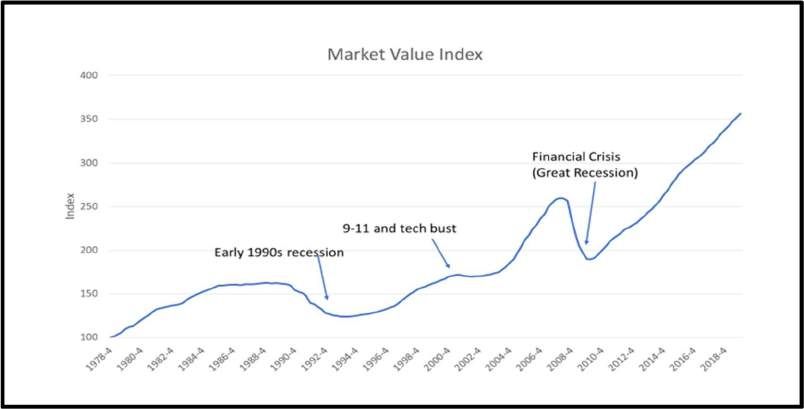
 14

estate for pension funds. The National Council of Real Estate Investment
 Fiduciaries (NCREIF) index is a widely used benchmark that tracks
 income and appreciation of institutionally owned commercial real estate
 (CRE). The quarterly data series starting in 1978 includes the
 performance of over 40,000 office, industrial, retail, multifamily and hotel
 properties plus other specialized property types such as self-storage and
 senior housing.
6.3 The following chart shows how the market value of NCREIF properties
 has changed over the past 42 years10. There is a parallel, albeit on a
 shorter time series, with the 400 years of data on housing prices in the
 Netherlands that we looked at earlier. We note that property values have
 increased over time despite intervening systemic shocks as evidenced
 by the rising market value index (MVI) over time. MVI is an equal
 weighted index which seeks to reduce the impact of value changes of
 large properties on the aggregate index. We observe that in each
 recession episode, value falls hit a floor, which is supported by the
 tangible value of real estate, and then rebound thereafter.

 Source: NCREIF & Jeffrey D. Fisher, Ph.D.

 15

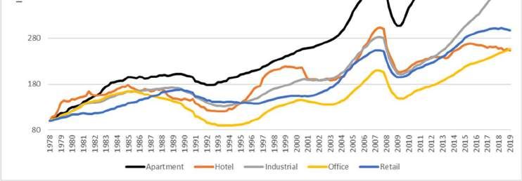
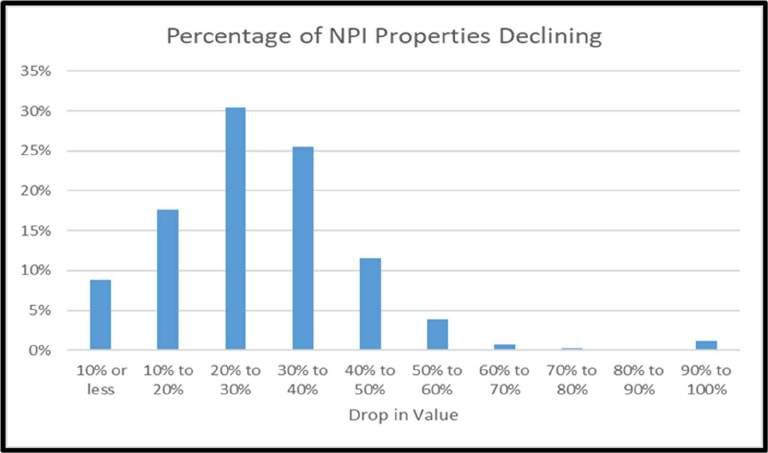
6.4 We have asserted that the tangible and intrinsic value of real estate
 provides a floor to the downside during period of declines. This makes
 the return distribution asymmetric and skewed right. Examining value
 declines in commercial property values as a result of the Global Financial
 Crisis lends light for this thesis. Looking at property value declines, peak
 to trough, using NCREIF data, we stratify the universe by percentage of
 declines. The following chart shows that the bulk of the declines ranged
 from 20%-40%10. Absent outliers, 50% value falls were the lower bound.

 Source: NCREIF & Jeffrey D. Fisher, Ph.D.

6.5 We asserted earlier that while real estate responds in aggregate to
 shocks, individual sectors of real estate respond differently and may in
 fact move more autonomously than the aggregate. The following chart
 shows the MVI index broken out by the five principal sectors, namely,
 apartments, hotel, industrial, office and retail10. We can see variability in
 value changes over time between each sector.

 16

Source: NCREIF & Jeffrey D. Fisher, Ph.D.

6.6 The following chart shows total returns of institutional real estate from the
 NCREIF (NPI index). Unlike the market value index, total returns in NPI
 include income returns in addition to appreciation. We note that the 1991
 Credit Crunch and Savings and Loans Crisis resulted in a real estate
 collapse. Total returns, meaning depreciation in property prices after
 factoring net income from rents, reached -13.4% in 1992. This was
 followed by 19 quarters of above 10% annualized total returns i.e.
 appreciation in property prices plus net income from rental revenues.
 The Global Financial Crisis resulted in a more severe real estate collapse
 which hit -26.7% in total annual return in 2009. This was followed by 23
 quarters of above 10% annualized returns in real estate. The anecdotal
 data suggests the larger the dislocation the stronger the ensuing
 performance in the long run.

 17

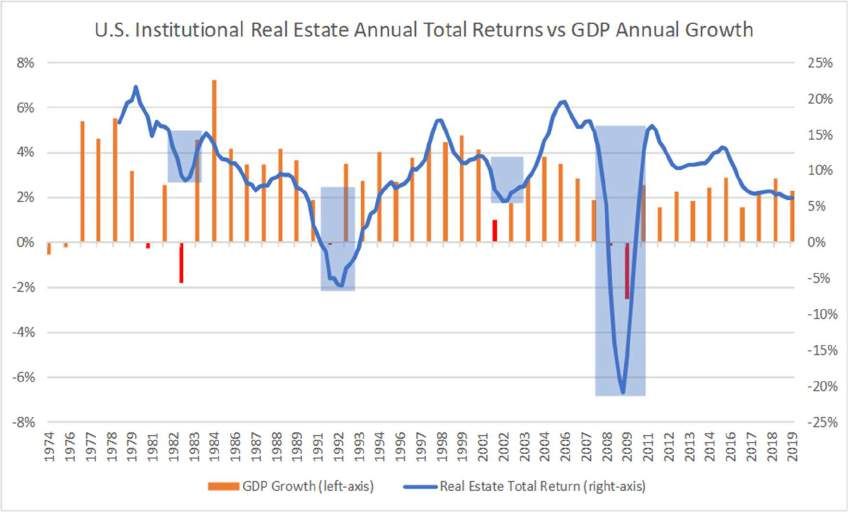
US Institutional Real Estate Total Returns
 25.0%

 20.0%

 15.0%

 10.0%
 19 quarters 23 quarters
 5.0%

 0.0%
 1979 1983 1987 1991 1995 1999 2003 2007 2011 2015 2019
 -5.0%

 -10.0%
 The bigger the Black Swan event the
 stronger the Returns
 -15.0%

 -20.0%
 Source: NCREIF NPI
 -25.0%

7. Empirical Data for Real Estate Convexity
 7.1 Thus far we have inferred convexity based on first principles effected by
 means of curtailment of new construction following market shocks. The
 slower it takes for new supply to return the longer rental pricing power
 favors owners. We also saw anecdotally that the length of real estate
 outperformance corresponds to the depth of the real estate decline
 following systemic shocks. We now seek to examine convexity
 empirically.
 7.2 A systemic shock refer to the widespread adverse impact on the financial
 system stemming from an unforeseen cause. The cause can be
 endogenous to financial market meaning that the shock was a result of a
 negative event triggered by a problem from within the financial industry.
 Or the cause may be exogenous where the source of the disturbance
 emanates from outside the field of finance. Terrorism, war, plagues are
 examples of exogenous shocks. The size of the adverse impact on real
 estate performance is a function of the type and severity of the shock.
 For the purposes of studying real estate’s antifragility we are less
 concerned with source of the shock and the immediacy of the decline in
 real estate values but we are focused on the length and strength of the
 recovery of real estate in the years following the shock.
 7.3 As a measure for Black Swan events or market shocks we use real GDP
 declines. We can see that real estate total returns are impacted by

 18

external shocks in the following chart. We use annualized total returns
 from the NCREIF return index on institutionally owned commercial real
 estate as a measure for real estate performance. We can see visually
 that each downturn is followed by a sustained period of strong real estate
 returns.

 Source: NCREIF

7.4 To test for convexity we need to plot real estate performance against
 volatility. We use annual percentage change in real GDP as a proxy for
 volatility. The bigger the shock the greater the downside to GDP growth.
 We compare a marked slowdown in GDP growth (which includes an
 outright recession) with the average level of GDP growth in the prior 2
 years. In the case of the 1982 recession we compared only against 1981
 as 1980 was also a recession year. In the case of 2001, while GDP
 growth was slightly positive, the less than 1% growth was a marked fall
 from the 4%+ growth in the prior 2 years. The 3% divergence in growth
 represented the effects of a shock which in this case was the 9/11 terror
 attacks.

 19

7.5 Following each episode of GDP volatility there followed a period of
 sustained real estate outperformance. We calculated the cumulative
 total returns using NCREIF performance data in each case. We then
 adjusted the returns by CPI to
 Severity of Cummulative
 obtain inflation adjusted or real
 Point GDP Shock Real Returns
 returns. We then plotted volatility
 C (1982) 4.34% 54.72%
 as measure by GDP declines A (1991) 2.89% 55.91%
 against the cumulative total real B (2001) 3.44% 56.40%
 returns from real estate following D (2008-09) 5.04% 80.76%
 each shock.
7.6 Can convexity be demonstrated empirically? In mathematics, based on
 Jensen’s inequality11, in order for function ( ) to be convex then
 ( ) { ( ) ( )}
 ≤ . We can apply this proof.

 7.6.1 ( ) = 55.91; ( ) = 80.76; ℎ = 2.89 = 5.04;
 { ( ) ( )} ( )
 ℎ = 68.33. = {3.96}

 From the chart we visually observe the {3.96} is in between point
 B and C. The result will be roughly 55 and will not be more than
 60. Since 55 60 < 68.33 the proof is valid. The points
 { ( ) ( )} ( )
 are indicated in the chart below. Clearly
 { ( ) ( )} ( )
 .

 7.6.2 ( ) = 56.40; ( ) = 80.76; ℎ = 3.44 = 5.04;
 { ( ) ( )} ( )
 ℎ = 68.57. = {4.24}

 From the chart we visually observe the {4.24} is in between point
 B and C. The result will be roughly 57 and will not be more than
 60. Since 57 60 < 68.57 the proof is valid.
 7.6.3 ( ) = 55.91; ( ) = 54.7; ℎ = 2.89 = 4.34;
 { ( ) ( )} ( )
 ℎ = 55.31. = {3.61}

 From the chart we visually observe the {3.61} is in between point
 B and C. Since the distance between B and C is fairly short, the
 result will on the line (more likely under the line) between B and C,
 which is congruent with line between A and D. (3.61} ≤ 55.31
 supporting the Jensen inequality for convexity.

 20

Cummulative Real Estate Total Returns Post Shock
 85%
 D
 Cummulative Total Real Returns

 80%
 75%
 70%
 {f(A)+f(D)}/2}
 65%
 60%
 A B
 55% C
 f{(A+D)/2}
 50%
 45%
 40%
 2.0% 2.5% 3.0% 3.5% 4.0% 4.5% 5.0% 5.5% 6.0%
 Severity of GDP Shock

7.7 Another feature of convexity is that the sum of ( ) + ( ) decreases by
 “smoothing” a and b together. ( ) + ( ) = 136.7. Smoothing a and b,
 we select B and C since both points are inside of A and D. ( ) + ( ) =
 111.1 which is smaller than ( ) + ( ) as expected, supporting the
 proof for convexity.
7.8 We approach convexity by attempting linear, superlinear and sublinear
 curves to fit the empirical distribution found above. We are not seeking
 a perfect fit but rather the shape of the curve with reasonable accuracy.
7.9 We started with a second order linear regression as shown in the
 following chart. The goodness of fit R2 at 0.9031 is very high for this
 superlinear model. While there may be other functions with superior
 goodness of fit, we are only seeking to determine the shape of the curve
 with reasonable accuracy.
7.10 For reference we attempted a 1st order linear regression and derived only
 0.56 for the R2. The linear model was significantly inferior to the
 superlinear model.
7.11 We then attempted a sublinear function which was the logarithmic
 regression. The slightly concave curve has an even lower R2 of 0.4982.
7.12 Based on the empirical data, the superlinear function had a goodness of
 fit that was far superior than either a linear or concave function. Based
 21

on this result, as well as the Jensen inequality proof detailed earlier, we
 conclude that the performance of real estate in the longer run is convex
 with respect to the severity of the perturbation in the economy brought
 about by a systemic shock or Black Swan event.
 Superlinear Convex Model Best Fit: ( ) = + + 

 Cummulative Real Estate Total Returns Post Shock
 85%
 D
 Cummulative Total Real Returns

 80% R² = 0.9031
 75%
 Superlinear: 2nd order
 70%
 polynomial convex
 65%
 60%
 A B
 55% C
 50%
 45%
 40%
 2.0% 2.5% 3.0% 3.5% 4.0% 4.5% 5.0% 5.5% 6.0%
 Severity of GDP Shock

 Sublinear Concave Model Best Fit: ( ) = . ln( ) + Linear Model Best Fit: ( ) = + 

 Cummulative Real Estate Total Returns Post Shock
 85%
 D
 Cummulative Total Real Returns

 80%
 75%
 R² = 0.4982
 70%
 Sublinear: Logarithmic concave
 65%
 60%
 A B
 55% C
 50%
 45%
 40%
 2.0% 2.5% 3.0% 3.5% 4.0% 4.5% 5.0% 5.5% 6.0%
 Severity of GDP Shock

8. Covid-19 Black Swan
 8.1 As of this writing, the Covid-19 pandemic has resulted in over 2 million
 confirmed cases and 134,000 deaths based on data from John
 Hopkins15. With infections several order of magnitude greater than

 22

confirmed cases and estimates of case fatality ratios of 1·4% [0·4–3·5]
 in those aged

that multi-asset portfolios would benefit from assets that have convexity
 and antifragile characteristics. We posit based on both first principles
 and empirical data that private equity real estate investments have these
 desired attributes. Since private equity real estate underpins real estate
 debt (private and public) and public traded REITs, the antifragility benefits
 can be found in varying degrees in all 4 quadrants of real estate.
 9.3 Current market turbulence brought about by the sudden impact of the
 coronavirus demonstrates vividly the impact of unknown unknowns on
 investment portfolios. Real estate’s track record through other shocks,
 asymmetrically skewed right return distribution, and antifragility in the
 longer run suggests performance of multi-asset portfolios will benefit from
 higher allocations to real estate.

Footnotes and References

1) Diversification Issues in Real Estate Investment, Michael Seiler, James Webb, Neil Myer. Journal of Real Estate
Literature. Vol. 7, No. 2 (July, 1999). Published by American Real Estate Society.

2) Spanning tests on public and private real estate. Kevin C.H. Chiang, Ming-Long Lee. The Journal of Real Estate
Portfolio Management, Vol. 13, No. 1 (2007), Published by American Real Estate Society

3) Time-Varying Diversification Effect of Real Estate in Institutional Portfolios: When Alternative Assets Are
Considered. Kathy Hung, Zhan Onayev and Charles C. Tu. The Journal of Real Estate Portfolio Management. Vol.
14, No. 4 (2008)

4) The Importance of Taleb’s System: From the Fourth Quadrant to the Skin in the Game. Branko Milanovic - 29
January 2018. Global Policy Journal, Durham University

5) Edge.org. The Fourth Quadrant: A Map of the Limits of Statistics by Nassim Nicholas Taleb, 14 August 2008.
Introduction by: John Brockman

6) How Much Data Do You Need? A Pre-asymptotic Metric for Fat-tailedness Nassim Nicholas Taleb Tandon School
of Engineering, New York University November 2018 Forthcoming, International Journal of Forecasting

7) Finiteness of Variance is Irrelevant in the Practice of Quantitative Finance Second version, June 2008 Nassim
Nicholas Taleb

8) Gold Republic, This Is What I Learned from Nassim Taleb. April 25, 2018 Olav Dirkmaat. (Olav Dirkmaat,
Professor in Economics, Business School of Universidad Francisco Marroquín).

9) Farnam Street, Nassim Taleb: A Definition of Antifragile and its Implications (2014)

10) Impact of Recessions on CRE Values: Lessons from the NCREIF Index. Jeffrey D. Fisher, Ph.D.
https://www.ncreif.org/globalassets/public-site/covid19/fisher-impact-of-recessions-on-cre-value-2020-03-24.pdf

11) IPE Real Assets, COVID-19: Immediate and long-term effects on RE could be substantial [corrected], Richard
Lowe, 17 March 2020

 24

12) A Visual Explanation of Jensen's Inequality, Article in The American Mathematical Monthly · October 1993
(DOI: 10.2307/2324783), Tristan Needham, University of San Francisco

13) Edge.org. Understanding is a Poor Substitute for Convexity (Antifragility), Nassim Nicholas Taleb. 12 December
2012.

14) The Lancet Infectious Diseases. Estimates of the severity of coronavirus disease 2019: a model-based analysis.
March 30, 2020. https://doi.org/10.1016/S1473-3099(20)30243-7

15) John Hopkins University and Medicine, Coronavirus Resource Center (https://coronavirus.jhu.edu/map.html)

16) Estimates of the severity of coronavirus disease 2019: a model-based analysis. MRC Centre for Global
Infectious Disease Analysis, Abdul Latif Jameel Institute for Disease and Emergency Analytics, and Department of
Infectious Disease Epidemiology, Imperial College London, London, UK. Published Online March 30, 2020
https://doi.org/10.1016/S1473-3099(20)30243-7.

17) The Institute for Health Metrics and Evaluation (IHME) UW Medicine, University of Washington (April 1, 2020)

18) Longer-run economic consequences of pandemics? Oscar Jorda, Sanjay R. Singh, Alan M. Taylor, (Federal
Reserve Bank of San Francisco and Department of Economics, University of California, Davis) March 2020

19) The Global Decline of the Natural Rate of Interest and Implications for Monetary Policy by Sungki Hong and
Hannah G. Shell. 2019, No. 4. Posted 2019-02-01© 2019, Federal Reserve Bank of St. Louis.

 25