Appendix A: Technological Innovation Activities in Britain and Other Western Countries (1400-1900)-A Quantitative Analysis
←
→
Page content transcription
If your browser does not render page correctly, please read the page content below
ppendix A: Technological Innovation
A
Activities in Britain and Other Western
Countries (1400–1900)—A Quantitative
Analysis
As has been shown in Chap. 2, as regards the scientific-technological innovation
rates, Europe outpaced China (and the East in general) in the fifteenth century—see
Fig. 2.6 (“Number of innovations in science and technology in Europe and China
per half a century, 900–1600 CE”), which supports our idea that the Industrial
Revolution started in Europe in the fifteenth century. It started in the belt that
included the Netherlands, Southern Germany, Northern Italy, as well as some parts
of France, Spain and Portugal. We suggest identifying the last third of the fifteenth
century and the sixteenth century as the initial phase of the Industrial Revolution.
During the sixteenth and the first half of the seventeenth century, the achievements
of different European countries were consolidating and diffusing, thus creating a
new foundation for growth. This phase of modernization (in terms of inventions)
can be subdivided into two subphases: the first was characterized by comparable
levels of technological innovation activities in a number of European countries; at
the second phase an undeniable lead belonged to Britain.
As regards technological innovation, a comparison of Britain with its European
neighbors very clearly shows that the British lead began to appear only in the second
half of the seventeenth century (Figs. A.2, A.3, A.4, A.5 and A.6; in Figs. A.4 and
A.5 this can be seen particularly well). Before that, Britain clearly lagged behind
Italy, Germany, and (for some period) the Netherlands. Thus, it is clear that during
the two initial centuries of the Industrial Revolution Britain absorbed the achieve-
ments of European societies, and only then it was able to start its own innovative
climbing. This British lead gradually grew until it reached its peak in the second
half of the eighteenth century. But this superiority could not continue too long.
Already in the first decades of the nineteenth century it became visible that some
other European countries and the USA were trying quite successfully to catch up
with Britain (Figs. A.6 and A.7), and in the second half of the nineteenth century
(from the 1860s) Britain ceased to be a technological leader, and its role in the
global technological invention process decreased from decade to decade. The tech-
nological leader role started to be performed by the USA (see Figs. A.7 and A.8).
© Springer International Publishing Switzerland 2015 167
L. Grinin, A. Korotayev, Great Divergence and Great Convergence,
International Perspectives on Social Policy, Administration, and Practice,
DOI 10.1007/978-3-319-17780-9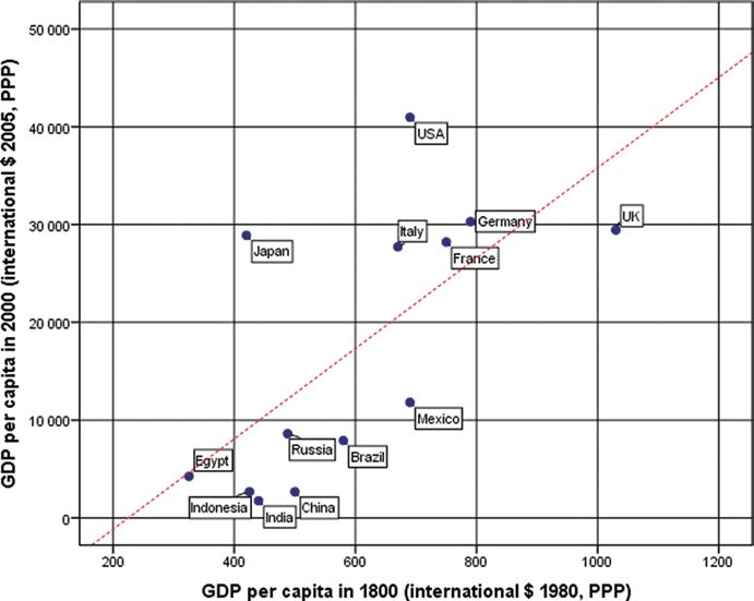
168                             Appendix A: Technological Innovation Activities in Britain...

   We emphasize again that, on the one hand, we see an evident technological
innovation leadership of Britain for two centuries (from the second half of the
seventeenth century to the first half of the nineteenth century); but, on the other
hand, for a greater part of this period, the overall innovation activity of “the rest of
the West” was higher than the one of Britain (Figs. A.9 and A.10). Thus, the primacy
of Britain in the technological invention field was relative, except for only one rela-
tively brief period of the second half of the eighteenth century and the early nine-
teenth century—i.e., the period of the final phase of the Industrial Revolution, when
the leadership of Britain was absolute (Figs. A.9 and A.10).
Methodology The main database used for calculations in this appendix is
Hellemans and Bunch (1988), which was augmented with data from Usher (1954),
Haustein and Neuwirth (1982), van Duijn (1983), Рыжов (1999), Silverberg and
Verspagen (2003), Ballhausen and Kleinelümern (2008), Challoner (2009) and
Kondratieff (1926, 1935, 1984). In this appendix we have only taken into account
technological inventions, excluding purely scientific discoveries (note that in
diagrams in Chap. 2 we try to quantify the innovation dynamics in science and
technology—hence, there we take into account both technological inventions and
scientific discoveries). In addition, in this appendix we take into account only those
inventions that were actually implemented within a century (thus, we do not take
into account those sketches of Leonardo da Vinci that remained on paper only).
With regard to scientific discoveries, the only exception was made to those of them
with a direct technological significance.
    For the initial phase of the Industrial Revolution and the first half of its interme-
diate phase (the fifteenth, sixteenth, and seventeenth centuries), we have identified
five major players in the technological innovation sector: Italy, Germany, France,
the Netherlands, and Britain (Figs. A.1, A.2, A.3 and A.4). Of course, some impor-
tant technological inventions were made in some other European countries (see
Figs. A.6, A.7 and A.8), and their total number exceeded in the fifteenth and six-
teenth centuries the one recorded for France. But in general, they did not play any
significant role until the early eighteenth century. Their role began to grow after-
wards, which confirms our idea of a common European space for open innovation
during the Industrial Revolution. Figures A.6, A.7, and A.8 clearly demonstrate that
in the eighteenth century the total number of major inventions made in the rest of
Europe (including Russia) exceeded the number of innovations in such a former
leader as Germany, in which the innovative activity in the technological area during
this time slowed down.
    For over a century and a half (until the early seventeenth century) Italy remained
the technological innovation leader. It also fully corresponds to an important fact
which was mentioned in Chap. 2—it is in Italy (especially in Venice) where in the
fifteenth and sixteenth centuries one could observe the most advanced legislation
and practice for registering inventions. However, the growth of its activity stopped
in the middle of the sixteenth century, while other countries were catching up with
Italy. The stagnation of the innovation activity in Italy correlated quite well with the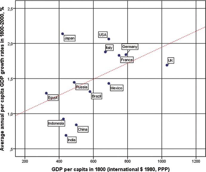
Appendix A: Technological Innovation Activities in Britain...                                       169

    14

    12

    10
                                                                                      Britain
     8                                                                                Italy
                                                                                      Germany
     6
                                                                                      France
     4                                                                                Netherlands
     2

     0
     1400         1450         1500         1550         1600         1650

Fig. A.1 Dynamics of technological inventions (=endogenous technological growth rate) in five
leading countries of Early Modern Europe, 1400–1650. Note: the data source is Hellemans and
Bunch 1988. Datapoints for 1450 refer to the fifteenth century, datapoints for 1550 refer to the
sixteenth century, datapoints for 1625 refer to the first half of the seventeenth century. The diagram
indicates the number of important technological innovations (listed in our database) made in
respective countries per century. If a database refers for half a century, we provide the endogenous
technological growth rate as inventions per century (to make all the datapoints comparable).
Hence, for the Netherlands, the datapoint for 1450 indicating “3” means that for the fifteenth cen-
tury our database lists three discoveries (which yields a “3 inventions per century” growth rate”),
for sixteenth century it increases to “4 per century”; for the first half of the seventeenth century our
database records six inventions in the Netherlands, which yields for the Netherlands for 1600–
1650 the endogenous technological growth rate of “12 inventions per century”

start of economic and political crisis, associated with changes of world trade routes,
its inability to change the political model of development and foreign policy chal-
lenges. At the same time, we note that future long-term leaders in innovation, Britain
and France at the start of the Early Modern Period were lagging far behind Italy and
Germany (Figs. A.1 and A.2, A.3 and A.4).
    Figures A.1, A.2, A.3, A.4 and A.5 indicate a rather interesting point, as in the
early seventeenth century four European powers converge as regards the number of
important innovations per country, which supports the idea that for the seventeenth
century it is quite possible to speak about a general Western European level of tech-
nological innovation activity. Although the further development of innovative activ-
ity in different countries was rather different, it is evident that a certain base was
established at a fairly high level, which was necessary to begin a new breakthrough,
a new phase of the Industrial Revolution. Also Figs. A.3 and A.4 show quite clearly
the stagnation of Italy, where in the seventeenth century the technological innovaton
activity rates fell almost to zero, which correlated quite well with the political and
social decline of Italy. Innovative activity from the south of Europe moved to the
North-West (including France) (see Fig. A.2).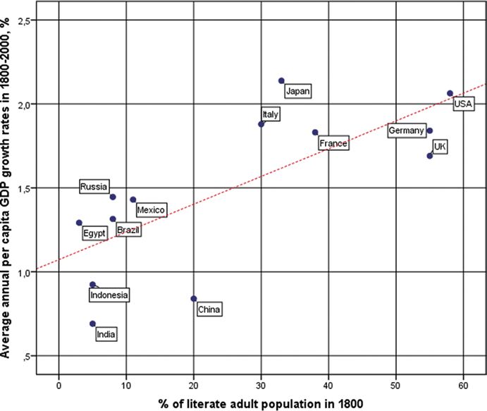
170 Appendix A: Technological Innovation Activities in Britain...
40
35
Britain
30
Italy
25
20 Germany
15
France
10
Netherlands
5
0
1400 1450 1500 1550 1600 1650 1700 1750
Fig. A.2 Dynamics of technological inventions (=endogenous technological growth rate) in five
leading countries of Early Modern Europe, 1400–1700. Note: datapoints for 1625 and 1675 refer
to the first and the second half of the seventeenth century respectively. Recall that in such cases we
still measure the endogenous technological growth rate as inventions per century (to make all the
datapoints comparable). Hence, for example, for the first half of the seventeenth century our data-
base records six inventions for Germany, which yields for Germany for 1600–1650 the endoge-
nous technological growth rate of “12 inventions per century”. For the second half of the
seventeenth century five major inventions are recorded in Germany, which yields for Germany for
1650–1700 the endogenous technological growth rate of “10 inventions per century”, etc
In the first half of the eighteenth century a certain divergence was observed in the
European North-West itself. The endogenous technological innovation rates grew
very substantially in France, but especially in Britain (see Fig. A.3).
Thus, already in the first half of the eighteenth century the British technological
lead became quite visible. But it only became really absolute in the second half of
the eighteenth century (see Fig. A.4).
As we see, in the second half of the eighteenth century in Britain the endogenous
technological growth rate increased by more than 250 %. This happened against a
rather slow growth of this indicator in France, a weak recovery in Italy and clear
decline in Germany and especially the Netherlands. As a result, the technological
lead of Britain became almost absolute—in the second half of the eighteenth century
the overwhelming majority of all the important technological inventions were made
in Britain (see Fig. A.9). The enormous lead of Britain with respect to the techno-
logical leaders of the start of the Early Modern Period becomes especially visible if
we delete the French curve from our graph (see Fig. A.5).Appendix A: Technological Innovation Activities in Britain... 171
40
35
Britain
30
Italy
25
20 Germany
15
France
10
Netherlands
5
0
1400 1450 1500 1550 1600 1650 1700 1750
Fig. A.3 Dynamics of technological inventions (=endogenous technological growth rate) in five
leading countries of Early Modern Europe, 1400–1750. Change of the leaders
140
120
Britain
100
Italy
80
Germany
60
40 France
20
Netherlands
0
1400
1450
1500
1550
1600
1650
1700
1750
1800
Fig. A.4 Dynamics of technological inventions (=endogenous technological growth rate) in five
leading countries of Early Modern Europe, 1400–1800. The absolute technological lead of the
British in the late eighteenth century172 Appendix A: Technological Innovation Activities in Britain...
140
120
Britain
100
Italy
80
60
Germany
40
Netherlands
20
0
1400 1450 1500 1550 1600 1650 1700 1750 1800
Fig. A.5 Dynamics of technological inventions (=endogenous technological growth rate) in four
leading countries of Early Modern Europe, 1400–1800. With France excluded the absolute techno-
logical lead of the British with respect to Germany, the Netherlands and Italy in the late eighteenth
century looks even more salient
However, this British absolute technological prevalence continued just for half a
century. Already in the first half of the nineteenth century the British endogenous
technological growth rate virtually stagnated against the background of a very fast
increase in those rates in France, Germany and the USA, as a result of which those
countries caught up with Britain in a rather significant way (see Fig. A.6), whereas
the number of major inventions made outside Britain exceeded substantially the
number of British inventions (Fig. A.10).
In the first half of the nineteenth century the Industrial Revolution was com-
pleted. Figures A.1, A.2, A.3, A.4, A.5 and A.6, as well as Figs. A.9 and A.10 in
different projections well confirm our idea that the Industrial Revolution from the
fifteenth to the nineteenth century passed through three phases: initial, intermediate,
and final.
In the second half of the nineteenth century Britain finally lost its technological
lead, as in the late nineteenth century the number of major inventions made in each
of the USA, Germany, and France exceeded the number of British inventions (see
Fig. A.7), whereas in 1880–1900 the number of major inventions made in Britain
constituted just about 10 % of all the major inventions made in the West (see
Fig. A.10). The technological lead by the end of the nineteenth century was clearly
taken by the USA (see Fig. A.7).Appendix A: Technological Innovation Activities in Britain... 173
140
Britain
120
100 Germany
80
France
60
Other
40 European
countries
USA
20
0
1400
1450
1500
1550
1600
1650
1700
1750
1800
1850
Fig. A.6 Dynamics of technological inventions (=endogenous technological growth rate) in
Europe and the USA, 1400–1850. A few Western countries are catching up with Britain in the first
half of the nineteenth century
300
Britain
250
200 Germany
150 France
100 Other
European
countries
50 USA
0
1450
1500
1550
1600
1650
1700
1750
1800
1850
1400
1900
Fig. A.7 Dynamics of technological inventions (=endogenous technological growth rate) in
Europe and the USA, 1400–1900. Convergence among the leading European countries and the
USA lead in the second half of the nineteenth century174 Appendix A: Technological Innovation Activities in Britain...
We continue to talk about the three phases of the Industrial Revolution as an
interconnected process, during which, however, technological leaders were changing,
which is quite clearly reflected in Figs. A.7 and A.8. At the initial phase (1450–1600),
we already see a fairly high rate of technological innovation activity (especially in
comparison with earlier periods that preceded the onset of the Industrial Revolution),
which further increased during the second half of the sixteenth century. This indi-
cates a transition to the intermediate phase when the base of the industrial revolution
greatly increased. As we remember (see Figs. A.1, A.2, A.3 and A.4), at this phase
technological leaders were Italy and Germany, but one could also observe a gradual
growth of the role of some other European countries: England, France and the
Netherlands. However, in the late sixteenth century it was not clear yet which coun-
try would be the future leader. The intermediate phase was characterized by the
emergence of new centers of technological innovation, as well as by the dissemina-
tion and improvement of previous innovations. Important improving inventions
were made, which were extremely important for the future of the Industrial
Revolution. The dynamics of the process was not linear, as the further development
of the technology base required a serious political change. This is quite visible in the
diagrams (e.g., Figs. A.3 and A.9). First, we see a general continuation of the inno-
vation activity growth in the first half of the seventeenth century (except Italy, which
in terms of invention rates stagnated—though still at a rather high level) and the
convergence of the endogenous technological growth rates on all the main countries
of Western Europe. In the second half of the seventeenth century in all the main
Western European countries (except Britain) the technological invention activity
stagnated or even decreased, yet it generally remained higher than at the previous
(initial) phase of the Industrial Revolution. In Germany, after a certain decline in
1650–1700, it somehow increased in the first half of the eighteenth century, but
Germany was no longer one of technological leaders of Europe. Real technological
innovation rise started there only in the first half of the nineteenth century. However,
during this period (the seventeenth century and the first half of the eighteenth cen-
tury) a number of important innovations in military tactics and strategy as well as in
international relations were made, which, however, by definition, we could not
reflect in our calculations. In any case, in the seventeenth century in Britain (not-
withstanding the political revolution and civil war) the technological invention
activity did not stagnate or decrease at all; what is more, it increased very signifi-
cantly, indicating the preparation of the technological breakthrough in Britain (to
some extent this was also a reflection of legislation on patents and monopolies that
was enacted in the early seventeenth century). Nevertheless, it is clear (see Figs. A.9
and A.10) that in the seventeenth century and even in the first half of the eighteenth
century, the total invention activity of Continental Europe was substantially greater
than the invention activity of Britain alone. In addition, two other new technological
innovation leaders emerged in the seventeenth century—the Netherlands and
France, which reflected the well-known World System hegemony of the Netherlands
in this century (see, e.g., Braudel 1981–1984; Arrighi 1994; Modelski 1987, 2006;
Modelski and Thompson 1996) as well as military-political growth of France [this,
in its turn, reflected the growing might of France as the leading continental power,Appendix A: Technological Innovation Activities in Britain... 175
300
Britain
250
Germany
200
France
150
Other
100
European
countries
USA
50
0
1750 1770 1790 1810 1830 1850 1870 1890
Fig. A.8 Dynamics of technological inventions (=endogenous technological growth rate) in
Europe and the USA, 1750–1900
140
120
100
80
Britain
60 Rest of the West
40
20
0
1400 1500 1600 1700 1800
Fig. A.9 Comparison of technological innovation rates in Britain and the rest of the West,
1400–1800176 Appendix A: Technological Innovation Activities in Britain...
800
700
600
500
400 Britain
Rest of the West
300
200
100
0
1400 1500 1600 1700 1800 1900
Fig. A.10 Comparison of technological innovation rates in Britain and the rest of the West in
1400–1900
which was the first in Europe to create a new type of state—a mature state (see
Гринин 2011; Grinin and Korotayev 2006; Grinin 2012a)].
Return now to the idea of comparing Britain with the rest of the West (Figs. A.9
and A.10). As we can see, before 1650 the number of major inventions made in
Britain was a few times less than in the rest of Europe; in 1650–1750 this gap
decreased very significantly, but still the number of major inventions made in the
Continent substantially exceeded the number of such inventions made in the British
Isles. We draw attention once again to the point that the overall growth of innovation
in Continental Europe slowed down very substantially in the period after the 30
Years War (and in Britain despite its revolution the technological innovation contin-
ued to accelerate). A new wave of invention activity growth started in the European
Continent in the first half of the eighteenth century (see Fig. A.9). However, in the
second half of the eighteenth century one could hardly observe in Continental
Europe anything comparable with the explosive growth of major technological
inventions that was observed in Britain during this period of time (corresponding to
the industrial breakthrough). In the second half of the eighteenth century Britain
became an absolute global technological leader, the main engine of world techno-
logical progress. But if we look at Fig. A.10, we can clearly see that in the overall
picture of the Industrial Revolution this is a relatively short period when Britain had
an almost total global superiority in the field of technological innovation, when
more technological inventions were made in Britain than in the rest of the world.
Already in the first half of the nineteenth century, a few Western countries managed
to catch up with Britain in a very significant way, and by the end of the nineteenth
century the USA, Germany, and France were outperforming Britain. Just becauseAppendix A: Technological Innovation Activities in Britain... 177 many countries of Continental Europe (as well as the USA) were ready to use those possibilities that were opened by the Industrial Revolution, this revolution was able to produce a world historical effect. So in conclusion, we note that the US coming to the first place with respect to technological innovation rates (Fig. A.8) meant not only the loss of leadership by Britain, but the fact of the formation of the West in the full modern sense of the word, of the West, which is not isolated only within Western Europe but includes North America, and Central Europe. And it meant the formation of the really well integrated World System.
 ppendix B: A Mathematical Model
A
of the Great Divergence and the Great
Convergence—Demography, Literacy,
and the Spirit of Capitalism

Reconsidering Weber1

In his classic The Protestant Ethic and the Spirit of Capitalism, Max Weber
(1904[1930]) suggested that Protestantism stimulated the development of modern
capitalism in Europe and North America. Weber disregarded the wide-spread expla-
nation of economic success of the Protestants in Europe in the Modern Age as a
result of their religious minority position. He pointed out that the German Catholics
failed to achieve similar results despite being a religious minority in many parts of
Germany.
    Weber explained the significant differences between Catholics and Protestants in
their social status and economic success by the different world views inherent in the
doctrines of these two confessions. He suggested that a decisive role was played by
the formation of a peculiar “spirit of capitalism”, which implied the devotion to one’s
business, the desire to increase one’s wealth in an honest way and so on. According
to Weber, the spiritual basis of capitalism was grounded in the vulgarized versions of
the theology of Calvinism and some other Protestant sects. It was, above all, the
belief in predestination and (in vulgarized versions) in the possibility to obtain the
signs of whether one is predestined to salvation via perfection in one’s profession.
    Many of Weber’s followers used to exaggerate the effect of religious ethics on
the economic dynamics. Yet, Weber himself wrote:
    “… however, we have no intention whatever of maintaining such a foolish and doctrinaire
    thesis as that the spirit of capitalism… could have only arisen as the result of certain effect
    of the Reformation, or even that capitalism as an economic system is a creation of the
    Reformation” (Weber 1930[1904]: 91).

1
 This section has been prepared on the basis of Chap. 6 of our monograph Introduction to Social
Macrodynamics: Compact Macromodels of the World System Growth (Korotayev et al. 2006a) that
has been written in collaboration with Daria Khaltourina.

© Springer International Publishing Switzerland 2015                                              179
L. Grinin, A. Korotayev, Great Divergence and Great Convergence,
International Perspectives on Social Policy, Administration, and Practice,
DOI 10.1007/978-3-319-17780-9
180 Appendix B: A Mathematical Model of the Great Divergence...
Yet, this doctrinaire thesis is still frequently attributed to Weber [see, e.g.,
Maddison (2001: 45), or Landes (1998)]. At the same time Weber, in our opinion,
showed quite convincingly that the processes of religious evolution could produce
some independent effect on socioeconomic development. On the other hand, the
mathematical model presented below in below in the section on “A Mathematical
Model of the Great Divergence and the Great Convergence” in the present suggests
another explanation for the correlation between the spread of Protestantism and
some increase in economic development, which was noted by Weber (see also
Korotayev et al. 2006a).
As is well known, the human capital development has been suggested as one of
the most important factors of economic growth, whereas education is considered to
be one of the most important components of human capital (see, e.g., Schultz 1963;
Denison 1962; Lucas 1988; Scholing and Timmermann 1988 etc.). We tested our
model below in the next section of the present Appendix and one of the assumptions
of this model was a significant positive effect of literacy level on the economic
growth during the modernization period. The model based on this assumption cor-
relates well with the historical data on the demographic, economic, and educational
dynamics of the World System (see below). Consequently, this hypothesis has
passed a preliminary testing. Let us also test it using cross-national data.
In the twentieth century, mass literacy spread around the globe, and nowadays
the differences in literacy levels between different countries tend to dissolve. At the
same time, according to our hypothesis, the differences in various countries’ eco-
nomic development during the process of Great Divergence were rooted in the
period of the beginning of modernization era. Therefore, it seems reasonable to
investigate the connection between such indicators as GDP per capita in 2000 and
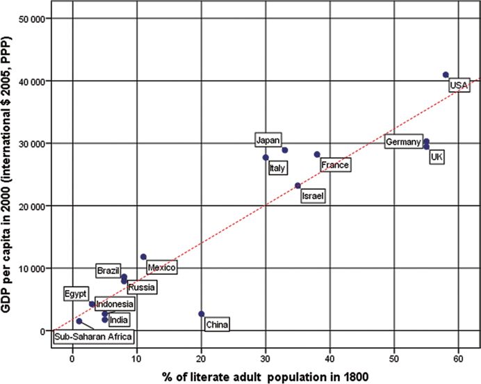
the literacy level in the early nineteenth century.2 For the data on these variables, as
well as on GDP per capita in the early nineteenth century, see Table B.1.
Note that a statistical test of this dataset generally supports Allen’s (2009, 2011)
hypothesis that the average income level in a country in the early nineteenth century
is regarded as the main predictor of its average income level around year 2000 (see
Fig. B.1).
As we see, in our case the correlation in the direction predicted by Allen’s
hypothesis, has again turned out to be quite strong (r = 0.65) and statistically signifi-
cant (p = 0.02).
However, what is even more important is that the per capita GDP levels in 1800
correlate positively and in a statistically significant way with the average annual per
capita GDP growth rates in the subsequent two centuries (1800–2000) (see Fig. B.2):
What is more, we believe that Allen’s explanation for this correlation is generally
accurate. In the nineteenth century, with the onset of intensive global modernization,
the countries with higher average per capita incomes (and, hence, with generally
higher wages) had more incentives to introduce new labor-saving (and, hence,
2
Since the indicators of educational level are strongly correlated with each other, the percentage of
literate population seems to be a good integral indicator of the level of education for the early
modernization period.Appendix B: A Mathematical Model of the Great Divergence... 181
Table B.1 GDP per capita in the countries and regions of the World in 1800 [international $ 1980,
PPP (Purchasing power parity)], GDP per capita in 2000 (international $ 2005, PPP) and % of
literate population in 1800
GDP per capita GDP per capita Average annual
in 2000 in 1800 per capita GDP % of literate
(international $ (international $ growth rates population
Country/Region 1995, PPP) 1980, PPP) in 1800–2000, % in 1800
USA 40,965 690 2.06 58
UK 29,445 1,030 1.69 55
Germany 30,298 790 1.84 55
France 28,210 750 1.83 38
Israel 23,213 (35)
Japan 28,889 420 2.14 33
Italy 27,717 670 1.88 30
China 2,667 500 0.84 20
Mexico 11,810 690 1.43 11
Brazil 7,906 580 1.31 8
Russia 8,613 488 1.45 8
India 1,745 440 0.69 5
Indonesia 2,679 425 0.92 5
Egypt 4,236 325 1.29 3
Sub-Saharan 1,502 (1)
Africa
Note: The source of the data on GDP per capita and literacy rate in 1800 is Мельянцев (1996); on
GDP per capita and the literacy rate in Russia in 1800 see Мельянцев (2003); on GDP per capita
in the countries and regions of the world in 2000 see World Bank (2014): NY.GDP.PCAP.PP.
KD. Our estimates are in parentheses
labor-productivity-increasing) technologies (that abundantly appeared in the nine-
teenth century); as a result, the productivity of labor (and hence, per capita GDP)
grew much faster in those countries than in the countries where the average incomes
(and wages) were lower (and where, as a result, the incentives to introduce labor-
productivity-increasing innovations were weaker), which, quite predictably, pro-
duced an unconditional divergence effect (Allen 2009, 2011).
However, we believe that this factor was not the only one. Below, we will discuss
another factor, which, as we will see, turns out to be much stronger than the one
proposed by Allen. And this factor is just the literacy level.
The correlation between literacy rates in 1800 and per capita GDP in 2000 is
presented in Fig. B.3.
Figure B.2 indicates that there is a very strong (r = 0.93) and definitely significant
(p ≪ 0.0001) linear correlation between the literacy rate in 1800 and GDP per capita
in year 2000. What is more, it is much stronger and more statistically significant
than the previous correlation (see Fig. B.1). R2 coefficient indicates that this corre-
lation explains 86 % of the entire data dispersion.
However, what is even more important is that the literacy rate in 1800 correlates
much stronger with the average annual per capita GDP growth rates in the subsequent182 Appendix B: A Mathematical Model of the Great Divergence... Fig. B.1 Correlation between per capita GDP in 1800 and per capita GDP Levels in 2000 (inter- national $ 2005, PPP), scatterplot with a fitted regression line. Note: r = 0.65, R2 = 0.42, p = 0.02 two centuries than the 1800 GDP per capita levels do (see Fig. B.4 and compare it with Fig. B.2). Therefore, the hypothesis that the spread of literacy was one of the major factors of modern economic growth gains additional support. On the one hand, literate populations have much more opportunities to obtain and utilize the achievements of modernization than the illiterate ones do. On the other hand, literate people are characterized by a greater innovative-activity level, which provides opportunities for modernization, development, and economic growth. Literacy does not simply facilitate the process of perceiving innovation by an individual. It also to a certain extent changes her or his cognition. This problem was studied by Luria, Vygotsky, and Shemiakin, the famous Soviet psychologists, on the basis of the results of their fieldwork in Central Asia in the 1930s. Their study shows that education has a fundamental effect on the formation of cognitive processes (perception, memory, and cognition). The researchers found out that illiterate respondents, unlike the literate ones, preferred concrete names for colors to abstract ones, and situative groupings of items to categorical ones (note that abstract think- ing is based on category cognition). Furthermore, illiterate respondents would fail
Appendix B: A Mathematical Model of the Great Divergence...                                       183

Fig. B.2 Correlation between per capita GDP in 1800 and average annual per capita GDP growth
in 1800–2000 (%), scatterplot with a fitted regression line. Note: r = 0.47, R2 = 0.22, p = 0.05
(1-tailed)

to solve syllogistic problems one of the kind: “Precious metals do not get rust. Gold
is a precious metal. Can gold get rust or not?” These syllogistic problems did not
make any sense to illiterate respondents because they were out of the sphere of their
practical experience. Literate respondents who had at least minimal formal educa-
tion solved the suggested syllogistic problems quite easily (Luria 1976; Лурия
1974, 1982: 47–69).
    Therefore, literate workers, soldiers, inventors and so on turn out to be more
effective than illiterate ones not only due to their ability to read instructions, manu-
als, and textbooks, but also because of the developed skills of abstract thinking.
Some additional support for this could be found in Weber’s work itself:
   The type of backward traditional form of labor is today very often exemplified by women
   workers, especially unmarried ones. An almost universal complaint of employers of girls,
   for instance German girls, is that they are almost entirely unable and unwilling to give up
   methods of work inherited or once learned in favor of more efficient ones, to adapt them-
   selves to new methods, to learn and to concentrate their intelligence, or even to use it at all.
   Explanations of the possibility of making work easier, above all more profitable to them-
   selves, generally encounter a complete lack of understanding. Increases of piece rates are
184 Appendix B: A Mathematical Model of the Great Divergence...
Fig. B.3 Correlation between literacy rates in 1800 (% of literate people among the adult popula-
tion) and per capita GDP levels in 2000 (international $ 2005, PPP), scatterplot with a fitted regres-
sion line. Note: r = 0.93; R2 = 0.86; p ≪ 0.0001
without avail against the stone wall of habit. In general it is otherwise, and that is a point of
no little importance from our view-point, only with girls having a specifically religious,
especially a Pietistic, background (Weber 1930[1904]: 75–76).3
We believe that the above mentioned features of the German female workers’
behavior simply reflect a relatively low educational level of German women from
labor circles in the late nineteenth—early twentieth centuries. The spread of female
literacy in Germany and elsewhere lagged behind the male literacy (see Korotayev
et al. 2006a, Chap. 7). In the early twentieth century, the majority of women could
write and read only in the most developed parts of Germany (Мельянцев 1996).
A more rational behavior of German workers from Pietistic circles could be easily
explained by the special role of education in Protestants’ lives.
The ability to read was essential for Protestants (unlike for Catholics) to perform
their religious duty—to read the Bible. The reading of Holy Scripture was not just
3
By the way, one can easily notice that these complaints on the working qualities of the German
women workers resemble very much the complaints on the working qualities of the Indian workers
made a few decades later and reported by Gregory Clark (2007: 353–357).Appendix B: A Mathematical Model of the Great Divergence... 185 Fig. B.4 Correlation between literacy rates in 1800 (% of literate people among the adult popula- tion) and average annual per capita GDP growth in 1800–2000 (%), scatterplot with a fitted regres- sion line. Note: r = 0.74; R2 = 0.54; p = 0.004 unnecessary for Catholic laymen, for a long time it was even prohibited for them. The edict of the Toulouse Synod (1229) prohibited the Catholic laymen from pos- sessing copies of the Bible. Soon after that, a decision by the Tarragon Synod spread this prohibition to ecclesiastic people as well. In 1408, the Oxford Synod absolutely prohibited translations of the Holy Scripture. From the very beginning, Protestant groups did not accept this prohibition. Thus, in 1522–1534, Luther translated into German first the New Testament and then the Old Testament, so that any German- speaking person could read the Holy Scripture in his or her native language. Moreover, the Protestants viewed reading the Holy Scripture as a religious duty of a Christian. As a result, the level of literacy and education was, in general, higher among Protestants than it was among Catholics and among the followers of other confessions that did not provide religious stimuli for learning literacy [see, for example: Малерб (1997): 139–157)]. In our opinion, this could to a considerable extent explain the differences between economic performance of the Protestants and the Catholics in the late nineteenth— early twentieth centuries in Europe noticed by Weber. One of Weber’s research goals
186                             Appendix B: A Mathematical Model of the Great Divergence...

was to show that religion can have an independent influence on economic processes.
The results of our study support this point. Indeed, the spiritual leaders of Protestantism
persuaded their followers to read the Bible not to support the economic growth but
for religious reasons, which were formulated as a result of ideological processes that
were rather independent of economic life. We do not question that specific features
of Protestant ethics could have facilitated economic development. However, we
believe that we found another (and probably more powerful) channel of Protestantism’s
influence on the economic growth of the Western countries.
    In the next section of this appendix we will try to use these findings in order to
develop such a mathematical model which is able to describe via six simple differ-
ential equations both the Great Divergence and the Great Convergence.

 Mathematical Model of the Great Divergence
A
and the Great Convergence4

In this section we suggest a simple mathematical model that is capable to describe
mathematically both the process of the Great Divergence and the one of the Great
Convergence.
   In this two-component model the world was divided into the core and the periph-
ery. The core includes high income OECD countries (the USA, Japan, Western
Europe, etc.). The periphery includes all other countries (except for post-socialist
countries of Eastern Europe and former USSR).
   For each of the two macro-zones the dynamics of three sub-systems are mod-
eled: (1) population; (2) technological-economic sub-system; (3) education-cultural
(human capital) subsystem. In initial conditions the level of the development of
sub-system 3 is set for the core to be significantly higher than the one in the periph-
ery. According to the model, the value of this variable affects positively the eco-
nomic growth and it affects negatively the population growth (reflecting the negative
impact of the female education on the fertility). On the other hand, the model
describes the technological transfer from the core to the periphery (the catch-up
term)—according to the model, the higher the level of the human capital in the
periphery, the easier the technological transfer takes place; on the other hand, the
larger is the gap between the core and the periphery, the higher is the value of the
catch-up term; hence, the catch-up force is very low at the initial phase with the very
low level of the human capital in the periphery, it becomes the highest at the
advanced phase when a wide gap between the core and the periphery is combined
with a rather high level of the human capital development in the periphery; and it
decreases again at the final phase with the decrease of the gap between the devel-
oped and developing countries.

4
 This section has been prepared on the basis of Chap. 2 of our monograph Mathematical Modeling
and Forecasting of the World and Regional Development (Коротаев и др 2010) that was written
in collaboration with Justislav Bogevolnov and Artemy Malkov (see also Zinkina et al. 2014).
Appendix B: A Mathematical Model of the Great Divergence... 187
Note also that within the model the population growth is assumed to be affected
positively by the economic growth, but, as the economic growth (both in the model
and the real life) also promotes the development of the education, finally it leads to
the decline of the population growth rates.
Within the model, at the first phase, the core’s GDP grows much faster than in
the periphery because of the high level of human capital in the core (which s timulates
the economic growth there) and the low level of human capital in the periphery
(which inhibits both the endogenous economic growth and the diffusion of the high
technologies from the core). Within the model this generates the Great Divergence.
Note that at this phase within the model the population in the core grows faster than
in the periphery, because the high economic growth rates outweigh there the influ-
ence of the education that is not high enough there to inhibit sufficiently the popula-
tion growth rates.
At the second phase, the economic growth rates in the periphery increase mainly
due to the development of the human capital there, as this promote both the endog-
enous economic growth and the transfer of the high technologies from the core.
However, at this phase the level of education in the periphery is not sufficiently high
to inhibit decisively the population growth and to raise the economic growth rates to
the core countries’ levels; hence, at this phase the economic growth in the periphery
leads to a very substantial population growth, but as regards the GDP per capita, the
gap between the core and the periphery continues to increase.
Finally, at the third phase, the human capital in the periphery develops to such an
extent that it allows simultaneously to achieve substantially high endogenous eco-
nomic growth rates, very high levels of technological transfers (reflected in the high
value of the catch-up term), and a significant slowdown of the population growth
rates. As a result, at the third phase, the GDP per capita growth rates of the periphery
start to exceed substantially the ones of the core—thus, the explicit Great
Convergence begins within the model (note that the model also describes the fourth
phase when the convergence rate slows down due to the decrease of the gap between
the developing and developed countries, which leads to the decrease of the value of
the catch-up term).
We start with the model (B.1)–(B.2)–(B.3) [for the description of its underlying
logic see Korotayev et al. (2006a: 81–91)]:
dN
= aSN (1 − L ) , (B.1)
dt
dS
= bLS, (B.2)
dt
dL
= cSL (1 − L ) . (B.3)
dt
N is the population, L is the proportion of literate population, S is the “surplus” per
capita product produced at the given level of technological development per capita188 Appendix B: A Mathematical Model of the Great Divergence...
over the subsistence level5; a, b, c are constants. As we have shown earlier, this
“macromodel describes rather well the modernization period, which appears to
reflect the fact that [in this period] the development of human capital became the
most important factor of economic development (see, e.g., Denison 1962; Schultz
1963; Scholing and Timmermann 1988; Lucas 1988 etc.)” (Korotayev et al.
2006a: 86).
The model also assumes that under certain conditions the periphery could “catch
up” with the center through the diffusion of the technologies developed in the cen-
ter (which actually proceeds along with the capital diffusion). Naturally, this phe-
nomenon cannot be regarded unilaterally, as the diffusion of capital and technology
to the periphery becomes possible only at both center’s economic benefit (con-
nected with the costs decrease) and at the appearance of a sufficient quantity of
literate labor force in the periphery. Quantitative feature of the “convergence force”
(C, “catch-up coefficient”) was chosen as follows:
Sc − S p
C= ⋅ Lp , (B.4)
Sc + S p
where
Sc is “surplus” GDP per capita over subsistence income in the core;
Sp is “surplus” GDP per capita over subsistence income in the periphery;
Lp is literacy rate in the periphery.
This equation reflects the following logic. On the one hand, the higher the difference
Sc − S p
in per capita incomes between the core and the periphery , the stronger the
Sc + S p
“convergence force”, as in this case the capital in the core has more incentives to
move the production from the very high-wage core to the very low-wage periphery
(together with investments and technologies). However, the strength of this force
also depends on the level of the development of the human capital (which is mea-
sured in our model through the literacy rate L). Hence, even with a very high value
Sc − S p
of the convergence force will be rather low with a very low value of Lp.
Sc + S p
This reflects the point that even if wages in a certain region are very low, invest-
ments and capitals will hardly move there if the level of the human capital develop-
ment is so low that it is unable to absorb the technologies moving from the core
[Clark (2007, 359f) describes rather vividly how this happened in reality]. Thus, in the
1950s and 1960s the wages in South Asia were much lower than in South Europe;
however, South Europe had at that time a much more developed human capital that
allowed absorbing technologies from the most advanced Western economies much
5
This level was estimated as 440 international Geary–Khamis 1990 dollars in purchasing power
parity (PPP); for the justification of this estimate see Коротаев et al. (2007: 59–60).Appendix B: A Mathematical Model of the Great Divergence... 189
50 000
5 000
USA
Italy
East Pakistan/Bangladesh
500
1950 1960 1970 1980 1990 2000 2010
Fig. B.5 Per capita GDP dynamics in the USA, Italy, and East Pakistan/Bangladesh in 1950–
2008, international $ 1990 at PPP. Data source: Maddison (2001) and (2010)
easier than this was possible in South Europe—hence, during those decades capitals
(and technologies) preferred to move to South Europe rather than to South Asia
(and the economic growth rates in South Europe were much higher than in South
Europe). On the other hand, by the 2000s the gap in the incomes between South
Europe and the most advanced Western economies had shrunk in a very substantial
way, remaining still very wide as regards South Asia6 (see Fig. B.5), whereas the
human capital had developed in South Asia by that time in a rather dramatic way
(see Figs. 3.3 and 3.4). Hence, it is not surprising that in the 2000s South Asia grew
much faster than the World System core in general, and South Europe in particular7
(see Fig. B.5).
Hence the gap between Sc and Sp continues to grow (the Great Divergence) until
the human capital development level of the periphery (Lp) reaches a certain level
after which the Great Convergence starts. Equation (B.4) seems to be the most par-
simonious way to describe mathematically the abovementioned pattern of the Great
Divergence and Great Convergence.
The model also accounts for the factor of resource limitations and fundamental
limitations (see Акаев 2010).
It should be noted that the accuracy of the mathematical description of the World
System macrodynamics regarded by the model significantly increases (especially
for the latest decades) if the model accounts for a 25 to 30-year-long lag between
literacy growth and the acceleration of economic growth rates. This is not surpris-
ing, as the databases that we used (first of all, ones affiliated with UNESCO) com-
monly regard literacy rate as the proportion of literate population aged 15+. That is
6
And—of course—the other Third World regions.
Sc − S p
7
Note that the highest values of the convergence force are observed when a large value of
Sc + S p
is accompanied by a very high level of the human capital development—this was just the case of
China in the recent decades.190 Appendix B: A Mathematical Model of the Great Divergence...
why literacy level growth (which has lately been proceeding almost only in the
Third World countries) occurs each year due to the increase in the proportion of
literate 15-year-olds (thanks to the gradual increase of primary education enroll-
ment rate).
However, the growth of the proportion of literate 15-year-olds does not lead to
any significant increase of economy growth rates, as even in modern developing
countries the majority of literate 15-year-olds do not get involved into manufactur-
ing, but continue their education (even if they start working in manufacturing, they
are likely to get only low-qualified jobs where their literacy does not lead to any
remarkable productivity growth). The effect of literacy rate growth within this given
age cohort is likely to reveal itself only in 25–30 years when the representatives of
this age cohort achieve the maximum level of their professional qualification.
Thus, the following lags were introduced into the model: 30 years between the
literacy growth and the corresponding GDP per capita growth, and 10 years between
the literacy growth and the corresponding slowdown of the population growth rates.
Since the late nineteenth century Kondratieff waves have been clearly observed
in time series, especially for economy growth rates (see, e.g., Kondratieff 1926,
1935, 1984; Schumpeter 1939; Rostow 1975; Mensch 1979; Forrester 1981; van
Duijn 1983; Marchetti 1986; Freeman 1987; Goldstein 1988; Berry 1991; Hirooka
2006; Tausch 2006; Papenhausen 2008; Korotayev and Tsirel 2010; Korotayev
et al. 2011d; Modelski 2012; Thompson 2012; Perez 2012; Grinin et al. 2012;
Korotayev and Grinin 2012a; Гринин and Коротаев 2012). Thus, Kondratieff
behavior with a 40 to 60-year-long period was externally introduced into the model.
In the wave dynamics downswing phases are 1929–1947 and 1973–1987, while
upswing phases are 1895–1929, 1947–1973, and 1987–2008.
The following equations are proposed for the formalization of what has been said
above. Let
Nc be population in the core, thousands
Sc be “surplus” GDP per capita in the core
Lc be literacy rate in the core
Np be population in the periphery, thousands
Sp be “surplus” GDP per capita in the periphery
Lp be literacy rate in the periphery
and the system of equation looks as follows:
dN c ( t )
= ac N c ( t ) Sc ( t ) (1 − Lc ( t − 10 ) ) + α N p ( t ) C ( t )
dt
dSc ( t ) G (t )
= bc Sc ( t ) Lc ( t − 30 ) 1 − K (t ) (B.5–B.7)
dt Glim
dL t
c ( ) = c L ( t ) S ( t ) (1 − L ( t ) ) K ( t )
dt c c c cAppendix B: A Mathematical Model of the Great Divergence... 191
dN p ( t )
= a p N p ( t ) S p ( t ) (1 − L p ( t − 10 ) )
dt
dS p ( t ) G (t )
= bp S p ( t ) L p ( t − 30 ) 1 − K ( t ) + β Sc ( t ) C ( t ) (B.8–B.10)
dt Glim
dL t
p ( ) = c L ( t ) S ( t ) (1 − L ( t ) ) K ( t ) + γ L ( t ) C ( t )
dt p p p p c
G = N c Sc + N p S p Global GDP, $ thousandsa
Sc − S p “convergence coefficient” describes the interaction of the two
C= ⋅ Lp components of the system
Sc + S p
Glim = 400 trillion dollars Fundamental limitation
K(t) Kondratieff dynamics
a
Following Angus Maddison (2001, 2010) calculations here and below are made in international $
1990, PPP
Thus, for each of the two macro-zones the dynamics of three sub-systems are
modeled:
–– population, Eq. (B.5) for the core, and Eq. (B.8) for the periphery;
–– technological-economic sub-system, Eq. (B.6) for the core, and Eq. (B.9) for the
periphery;
–– education-cultural subsystem, Eq. (B.7) for the core, and Eq. (B.10) for the
periphery.
Table B.2 states the values of equations’ coefficients and initial values of the
variables N, S, and L (for 1800):
The component αNpC describes the migration from the periphery to the core,
while the migration from the core to the periphery is negligible. We suppose that the
volume of migration is proportionate to the periphery literacy rate and to GDP per
capita discrepancy between the core and the periphery (as it is mostly literate people
in search for better lives who migrate).
The component βScC describes the diffusion of capital and technology to the
periphery. We suppose that both capital and technology start flowing actively
only at a sufficient literacy level of the interacting regions (this is why C is
Table B.2 Values of equations’ coefficients and initial values of basic variables
“Convergence
Core Periphery coefficient”
ac 2.1 × 10⁻⁵ Nc 1.6 × 10⁵ ap 3.3 × 10⁻⁵ Np 9.0 × 10⁵ α 4.0 × 10⁻⁴
bc 2.7 × 10⁻² Sc 580 bp 3.7 × 10⁻² Sp 120 β 4.0 × 10⁻³
cc 1.4 × 10⁻⁵ Lc 0.42 cp 5.0 × 10⁻⁶ Lp 0.10 γ 1.0 × 10−8192 Appendix B: A Mathematical Model of the Great Divergence...
included into Lp), as well as with a sufficient GDP per capita discrepancy S
between the regions.
The component γLNpC describes literacy diffusion to the periphery.
The second equations of the system (dynamics of S) are to be regarded sepa-
rately. Taagepera-Kremer-Tsirel-Jones equation looks like
dT
= bNT .
dt
It describes the dynamics of technology development. Taagepera (1976, 1979,
2014), Kremer (1993), Tsirel (2004), and Jones (2005) suppose that the relative
technology growth rates are proportionate to population number: the more people,
the more potential inventors. It should be accounted here that Taagepera, Kremer,
Tsirel, and Jones imply summing the innovation, i.e., not only that a larger number
of people do produce more innovations, but they produce more complementary
innovations, not repeating ones. This is possible only if the mass of people repre-
sents a coherent system. Taagepera, Kremer, Tsirel, and Jones regarded the equation
for the World System and stated that it would not work for its separate parts (see
also Korotayev 2005, 2007, 2008, 2009, 2012; Korotayev et al. 2006a, b; Korotayev
and Khaltourina 2006; Khaltourina and Korotayev 2007).
Indeed, as we have seen above, the periphery having a much larger population did not
produce a larger number of innovations than the core. Among other circumstances it was
connected with the fact that the periphery did not represent a holistic system, and did not
“sum up” its inventions: the innovations made in Africa did not contribute to the innova-
tions in Latin America, neither did they improve the living standards in South Asia.
With regard to this we proposed an alternative equation for technology growth
which in our model is associated with S:
dS
= bSL.
dt
The growth rates of technology and GDP per capita are proportionate to literacy rate.
Thus, we suppose that namely literacy provides for the additivity of innovations.
From the point of view of the basic one-component model of the World System
development, replacing N for L does not “spoil” the dynamics, because, as we have
seen above, N is proportionate to L almost in the whole diapason of the demo-
graphic transition (see Korotayev et al. 2006a, b for more details).
Retrospective Numerical Calculation from 1800 till the 2000s
Figure B.6 presents the results of quantitative calculation for the period from 1800
till the 2000s:
Figure B.7 describes the dynamics of the difference between the core and the
periphery as regards per capita GDP. Figure B.8 presents economic growth rates of
the core and the periphery.Appendix B: A Mathematical Model of the Great Divergence... 193
Core Periphery
0.9 7
0.8 6
0.7
Population
5
(billions)
0.6
0.5 4
0.4 3
0.3 2
0.2 1
0.1 0
1800 1850 1900 1950 2000 1800 1850 1900 1950 2000
sands of inter-national
30 5
PercapitaGDP (thou-
4.5
25
4
20 3.5
3
dollars*)
15 2.5
10 2
1.5
5 1
0.5
0
1800 1850 1900 1950 2000
1800 1850 1900 1950 2000
100 100
80 80
Literacy (%)
60 60
40 40
20 20
0
0
1800 1850 1900 1950 2000
1800 1850 1900 1950 2000
Fig. B.6 Parameters of order. Empirical and theoretical curves. Note: Constant international $
1990, PPP. Here and below black curves stand for the calculation, while grey marks represent
historical data
Fig. B.7 Difference between 10
the core and the periphery
with respect to per capita 9
Numerical
GDP. Note: the figures on the calculation
8
Y-axis scale denote by how
many times the GDP per Historical data
7
capita in the developed
countries exceeded that in the 6
developing countries for a
given year. Thus, the value of 5
7 for 1960 means that in 1960
the GDP per capita was in the 4
developed countries seven 3
times as high as in the
developing countries. Source 2
of historical data: Maddison
(2010) 1
0
1800
1820
1840
1860
1880
1900
1920
1940
1960
1980
2000194 Appendix B: A Mathematical Model of the Great Divergence...
Core Periphery
6 8
5 7
Annual GDP growth rate (%)
6
4 5
3 4
3
2 2
1 1
0
0 –1
1800 1850 1900 1950 2000 1800 1850 1900 1950 2000
6 6
5 5
Annual per capita GDP
4 4
growth rate (%)
3 3
2 2
1 1
0 0
–1 –1
1800 1850 1900 1950 2000 1800 1850 1900 1950 2000
Fig. B.8 Indicators of economic growth rates. Empirical and theoretical curves
Forecast
The model check on the basis of historical data shows that it describes rather accu-
rately the main trends connecting such key variables of the global dynamics as the
world population, GDP, and education. This result allows us to use the model not
only in retrospective, but also for forecasting as well. The forecast horizon was
chosen as half a century, as this is the characteristic time scale for the variables
specified. The results of the calculations made according to the model allow making
the following forecast (see Figs. B.9 and B.10).
The diagrams suggest that the Great Convergence process will continue in the
forthcoming decades, though its rate will experience a certain slowdown.8
One of the most important results of the proposed forecast looks as fol-
lows. Our inertial9 population forecast exceeded significantly the UN medium
8
In the real world this may be connected with the prospect of the “Reindustrialization of the West”,
on the one hand, and the “middle income trap” threatening the development of many middle-
income countries, on the other. As defined by Aiyar et al., the “middle-income trap” is “the phe-
nomenon of hitherto rapidly growing economies stagnating at middle-income levels and failing to
graduate into the ranks of high-income countries” (Aiyar et al. 2013: 3). For a detailed description
of the factors and mechanisms of the middle income trap see, e.g., Kharas and Kohli (2011). In
general the model predicts the slow-down of the Great Convergence speed with the decrease of the
gap between the First and the Third World in the forthcoming decades.
9
The inertial forecasts were generated by the mathematical model (4)–(9) with those values of
parameters that produced the best fit with the empirical data for the last two centuries.You can also read