Assessing claims made by a pizza chain
←
→
Page content transcription
If your browser does not render page correctly, please read the page content below
Journal of Statistics Education, Volume 20, Number 1(2012)
Assessing claims made by a pizza chain
Peter K. Dunn
University of the Sunshine Coast
Journal of Statistics Education Volume 20, Number 1 (2012),
www.amstat.org/publications/jse/v20n1/dunn.pdf
Copyright © 2012 by Peter K. Dunn all rights reserved. This text may be freely shared among
individuals, but it may not be republished in any medium without express written consent from
the author and advance notification of the editor.
Key Words: Initial data analysis; t-tests; Boxplots; Study design; Real data
Abstract
A pizza chain in Australia made a number of claims about the size of its pizzas relative to those
from another pizza chain. Interestingly, the pizza chain made publically available the data upon
which those claims were made. The claims of the pizza company can be assessed using these
data. Instructors can use the data to guide students to form research questions and hypotheses; to
produce numerous graphical, numerical and tabular summaries; and for conducting some simple
analyses such as one- and two-sample t-tests. Notes are made on how the data can be used to
demonstrate the importance of initial data analysis, and the importance of understanding the
source of the data and the research design. In addition, suggestions are made for how students
can use these results in a way that taps students‟ creative potential.
1. Introduction
Most statistical educators are aware of the value of using real data in classes, which has been
reinforced by the American Statistical Association‟s Guidelines for Assessment and Instruction
in Statistics Education in their College Report (Aliaga, Cobb, Cuff, Garfield, Gould, Lock,
Moore, Rossman, Stephenson, Utts, Velleman, and Witmer 2010). Using real data is advocated
for numerous reasons. Using real data:
Demonstrates to students the relevance and importance of statistics in solving real (not artificial)
problems (Hand, Daly, Lunn, McConway, and Ostrowski 1996; Bradstreet 1996);
Emphasizes that statistics is not just about computation, but about solving real problems (Hand et
al. 1996), which can increase student interest and engagement in the analysis and the use of
statistics (Aliaga et al. 2010);
Ensures students do not perpetuate the idea that statistics is dull and dry (Willet & Singer 1992);
1Journal of Statistics Education, Volume 20, Number 1(2012)
Ensures the data are realistic and not misleading, and do not misrepresent the context (Hand et al.
1996; Aliaga et al. 2010);
Engages students in thinking about the data and related statistical context (Aliaga et al. 2010) and
adds value to statistical thinking (Bradstreet 1996);
Enables students to learn to formulate good research questions, and be able to use the data to
answer these questions (Aliaga et al. 2010); this helps students to understand why we analyze
data, not just how (Willet & Singer 1992);
Ensures students remember the analysis as one that solved a real problem (Bradstreet 1996);
Can be memorable, becoming triggers for later recall of the statistical techniques (Singer &
Willet 1990);
Validates the importance of exploratory (or initial) data analysis (Singer & Willet 1990).
No doubt, other reasons can also be found. In summary, as is often quoted, “If you have only
pretend data, you can only pretend to analyze it” (Watkins, Scheaffer and Cobb 2004, page vii).
Willet & Singer (1992) lists eight attributes of real data that make such data effective for
teaching: the data are in raw form; are authentic; include sufficient background information;
have case-identifying information; are interesting or relevant to students; are topical or
controversial; offer substantive learning; and lend themselves to many analyses.
While the use of real data is admirable for all the reasons listed above, fake data can also be used
effectively for many situations (for example, the famous Anscombe (1973) datasets). In fact,
Gelman & Nolan (2002, p. 3) even state that “it can be good to use fake data for a first example
and to discuss how you set up the fake data and why you did it the way you did.”
Sources of real data are numerous. There are many books (for example, Hand et al. 1996;
Chatterjee, Handcock, and Simonoff 1995; Peck, Haugh, and Goodman 1998; Peck, Casella,
Cobb, Hoerl, Nolan, Starbuck, and Stern 2006) and websites (such as, OzDASL, Smyth 2011;
the JSE Data Archive, American Statistical Association 2011; The Data and Story Library 1996)
that offer access to real data sets. These resources make the task of finding suitable real datasets
far easier and quicker.
While the use of real data is pervasive and advantageous,
…real data problems are necessary but not sufficient. It is not enough to have “data
examples.” Considerable care and some skill are needed to use the full data problems to
communicate the entire process of data analysis and the role of statistics in scientific
learning. (Schafer and Ramsey 2003, Section 3)
A further challenge exists when teaching large, first-year statistics classes to students enrolled in
a wide range of disciplines: finding real datasets that appeal to the majority of students can be
difficult. The GAISE report (Aliaga et al. 2010, p. 16) acknowledges this when it states that
“few data sets interest all students, so one should use data from a variety of contexts.”
Recently, the author found a dataset that has the potential to appeal to a wide cross-section of the
usual university cohort, allows students to use some basic statistical skills taught in the typical
2Journal of Statistics Education, Volume 20, Number 1(2012)
introductory statistics course (exploratory skills and inference skills), but also raises a number of
questions about the study design and reporting that moves beyond just analysis.
Eagle Boys is a pizza chain in Australia that has, for many years, conducted an advertising
campaign that claims their large pizzas are bigger than those of Australia‟s largest pizza chain,
Domino‟s Pizza. This campaign strategy has adopted many forms. The current campaign
includes a webpage (http://www.eagleboys.com.au/realsizepizza, accessed 19 February 2012;
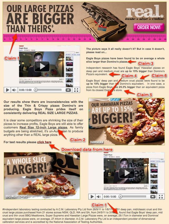
one page is shown in Figure 1), which makes a number of claims about the pizzas from both
companies:
Claim 1: The main claim in the advertisement is that “Our large pizzas are bigger than
theirs”. This is expanded upon in the fine print in the advertisement: “…Eagle Boys‟
deep pan, mid crust and thin crust BBQ Meatlovers, Super Supremo and Hawaiian Large
Pizzas were, on average, 29.17cm in diameter and Dominos‟ equivalent large pizzas
were, on average, 27.44cm in diameter.”
Claim 2: Eagle Boys‟ claim that they have “real size 12-inch large pizzas”.
Claim 3: “Eagle Boys pizzas have been found to be on average a whole slice larger than
Domino‟s pizzas.”
Claim 4: “Independent research has found Eagle Boys‟ Hawaiian pizzas on deep pan and
medium crust are up to 15% bigger than Domino‟s Pizza‟s equivalent.”
Claim 5: “In one case, a pizza from Eagle Boys was 25.3% bigger than an equivalent
pizza from its closest Domino‟s store.”
Claim 6: “Eagle Boys‟ deep pan and medium crust pizzas were found to be up to 10%
bigger than the Domino‟s equivalent.”
Helpfully, the previously-mentioned webpage points to the data upon which these claims are
based. This means that the claims made by Eagle Boys can be verified, at least potentially.
Other questions of interest can be studied also, some arising from the data and some from the
way in which the data are interpreted and used in the advertising.
In this article, the data are discussed (Section 2), including design issues (Section 3). This is
followed by a study of Claims 1 and 2 in some detail (Section 4). Then, further pedagogical uses
of the data, including the remaining claims, are discussed (Section 5).
3Journal of Statistics Education, Volume 20, Number 1(2012)
Figure 1: One page of the Eagle Boys campaign webpage, showing claims made by Eagle Boys (located
at http://www.eagleboys.com.au/realsizepizza, visited 19 February 2012)
4Journal of Statistics Education, Volume 20, Number 1(2012)
2. The data
The data were obtained by following the links in the webpage advertisement; the data are
publically available in a PDF file, but are undocumented. The data obtained in this manner also
contains numerous other variables whose descriptions were unclear. The author contacted the
independent company responsible for the testing (A.C.M. Laboratory Pty Ltd) as given on the
webpage, and an A.C.M. company representative replied saying “we just measured the
diameters” (Carol Sieker, personal communication in an e-mail dated 24 July 2011). Our request
for more information was then passed to Eagle Boys, both from the author directly and via
A.C.M., but no reply has been forthcoming. Consequently, the data made available here do not
include these variables whose meanings are unknown.
The data can be accessed in a comma-delimited file at:
http://www.amstat.org/publications/jse/v20n1/dunn/pizzasize.csv.
A documentation file for the data set can be accessed in a text file at:
http://www.amstat.org/publications/jse/v20n1/dunn/pizzasize.txt.
The data contain information from 250 pizzas, 125 each from Eagle Boys and Domino‟s. A
fuller description is provided in the Appendix A, and in Table 1. The data contain no missing
values. However, the data file contains an ID for each pizza tested, and all information regarding
IDs 192 and 193 are missing (so that the largest ID in the file is 252).
Helpful Hint: As a lead-in to the data, consider asking students to guess the mean size of
a large pizza, and then to guess the amount of variation observed in the sizes of large
pizzas.
3. Design and introductory issues
The claims made by Eagle Boys are a starting point for discussing these data. Students can be
engaged with the context by asking how they think the claims made on the campaign webpage
were substantiated.
Helpful Hint: Before revealing to the students that the data are available, ask students to
discuss how the claims could be tested. Ask students how such a study would be
designed, what data would be needed, etc., so they obtain some insight into the context.
A representative from the independent company who measured the pizza diameters told us that
“we weren‟t involved in the design of the experiment or the statistical analysis” (Carol Sieker,
personal communication in an e-mail dated 24 July 2011). In other words, their involvement
was simply measuring pizza diameters. Importantly, this means that no information is available
about how the pizzas in the data were selected.
Helpful Hint: This is an opportunity to talk about study design issues. For example, this
is an opportunity to talk about evaluating published studies, and self-funded studies in
5Journal of Statistics Education, Volume 20, Number 1(2012)
particular. Eagle Boys have funded the study, and presumably selected the samples sent
to A.C.M., and performed the analysis. How does this, and should this, affect our
perception of the conclusions?
The data give the pizza diameters in centimetres (one inch is 2.54 centimetres exactly). The data
as provided also contain the descriptions of the crust types as used by each company, which are
not always the same. Both companies use the “Deep Pan” description, but different terms for
the thinnest crust (“Thin „n‟ Crispy” for Domino‟s; “Thin Crust” for Eagle Boys) and the
medium crust (“Classic Crust” for Domino‟s; “Mid Crust” for Eagle Boys). We adopted the
terms Thin, Mid and DeepPan. Similarly, Domino‟s has a Supreme pizza, and the Eagle
Boys equivalent is called a Super Supremo, both of which we call Supreme.
Helpful Hint: We purposely do not amend these descriptions in the data files we make
available to students. (Other instructors may elect to make these changes before giving
the data to students.) Changing the descriptions to a common lexicon serves as a useful
reminder to the students that ‘real data’ usually needs cleaning and checking. The actual
task of making the amendments for these data is simple, so that the reminder can be made
without requiring the students to spend lots of time on the process of amending the data
itself.
4. Claims 1 and 2
4.1 Initial data analysis
Before testing any of the claims, an initial data analysis should be performed, consistent with
standard statistical practice. A variety of exploratory techniques can be employed to understand
the data, including graphics (for example, bar charts of toppings; boxplots comparing diameters
for each company), numerical summaries (means; etc.), two-way tables (for example, company
and crust; crust and topping; company and the number of pizzas exceeding 12-inches in
diameter). A numerical summary of the data is provided in Table 1.
Table 1: A numerical summary of the data. Diameters are given as mean (standard deviation) in
centimetres. (Note: Twelve inches corresponds to 30.48cm.)
Domino‟s Eagle Boys
Diameter n Diameter n
Crust Deep Pan 26.69 (0.46) 40 29.09 (0.48) 43
Mid 26.75 (0.51) 42 28.78 (0.48) 43
Thin 28.81 (0.80) 43 29.70 (0.55) 39
Topping BBQ Meatlovers 27.36 (1.16) 43 29.16 (0.56) 42
Hawaiian 27.36 (1.23) 41 29.21 (0.62) 43
Supreme 27.61 (1.13) 41 29.15 (0.71) 40
Combined 27.44 (1.17) 125 29.17 (0.63) 125
6Journal of Statistics Education, Volume 20, Number 1(2012)
The distributions of pizza diameter can also be explored graphically. A naïve plot comparing the
distribution of pizza diameters for each company (Figure 2) shows that Domino‟s pizzas tend to
have smaller diameters than those from Eagle Boys, and that the variability is much greater. A
more careful initial data analysis would also explore the relationships between the company and
pizza diameter for various crust types (Table 1; Figure 3) and toppings (Figure 4). These plots
reveal that the variation of the diameters across crust types is reasonably uniform for both
companies, but deep pan and mid crust pizzas from Domino‟s appear smaller in diameter than
those from Eagle Boys.
Figure 2: The distribution of the pizza diameter by pizza company. The gray horizontal line indicates 12
inches (30.48 cm).
Figure 3: The diameter of pizzas at both companies, for the three crust types.
7Journal of Statistics Education, Volume 20, Number 1(2012)
Figure 4: The diameter of pizzas at both companies, for the three toppings.
4.2 Claim 1
Claim 1 makes claims about the diameter of the pizzas in a very general sense: “Our large pizzas
are bigger than theirs”. This claim could be interpreted as a formal hypothesis test of H0: EB ≤
D against H1: EB > D where represents the mean diameter of the pizza. Using Welch‟s two-
sample t-test (t = 14.6; df = 189.8; one-tailed p < 0.0001) suggests strong evidence to reject the
null hypothesis. However, the initial data analysis indicates that this is an inappropriate
approach: the data should not be combined over crust types. Furthermore, the data contain a
number of outliers. The fine print in the advertisement implies a two sample t-test is the
approach taken, as the fine print quotes (correctly; see Table 1) the mean overall diameters for
both companies‟ pizzas.
Potential Pitfall: In R, which we used for analysis, the order of the two groups is (by
default) in alphabetical order. In other words, by default R will test the hypotheses H0:
D ≥ EB against H1: D < EB. Other software may approach hypothesis tests in a
similar way. Students and instructors should be wary of the output, and ensure that the
output matches the hypothesis being tested.
Helpful Hint: The implication in the claim is that a test for the comparison of means
should be one-sided. Consider asking students to justify whether the test should be one-
tailed or two-tailed.
If this analysis is inappropriate, it is possible that another analysis was used to substantiate the
claim? This is unlikely given the overall means quoted in fine print attached to the claim.
However, one possible alternative is that the claim has been substantiated by comparing the
pizza diameters within each crust–topping combination (that is, 3 3 = 9 individual Welch‟s two
8Journal of Statistics Education, Volume 20, Number 1(2012)
sample hypothesis tests provided evidence that Eagle Boy‟s pizzas had a larger mean diameter in
each subgroup). In each subgroup the results are statistically significant, but clearly a problem of
multiple testing is apparent. After adjusting using (for example) the method due to Holm (1979),
each sub-group comparison remains statistically significant (Table 2). While unlikely that such
analyses were performed, these results do support the overall claim made in the advertisement.
Table 2: The diameter of pizzas at both companies, for the three toppings.
Topping Crust Mean (Std dev) of the pizza p-value p-value (adj.
diameters (in cm) with “Holm”)
Domino‟s Eagle Boys
BBQ Thin 28.86 (0.62) 29.70 (0.48) 0.0004 0.0011
Meatlovers n = 14 n = 12
Mid 26.62 (0.44) 28.88 (0.30)Journal of Statistics Education, Volume 20, Number 1(2012)
In summary, evidence exists to support Claim 1 that Eagle Boys pizzas are significantly larger
than Domino‟s pizzas on average, but no evidence exists to support Claim 2, that the “real 12-
inch large pizzas” from Eagle Boys have a mean diameter of 12-inches. The campaign focuses
on the former result, despite the results probably being based on inappropriate analysis. It is
interesting that Claim 2 is even mentioned given that no evidence exists in support.
5. Further analysis using the data
5.1 Other claims
In this section, we make brief notes about assessing the other claims made by Eagle Boys.
First, consider Claim 3: “Eagle Boys pizzas have been found to be on average a whole slice
larger than Domino‟s pizzas.” On one level, this claim is silly: both pizzas have eight slices!
Helpful Hint: Instructors may take this opportunity to talk to students about clarity in
operational definitions and interpretations.
Presumably Claim 3 is made about the area of the pizzas, a claim that can also be tested. The
hypothesis is that the mean area of an Eagle Boy‟s pizza is at least the same as nine-eights of the
mean area of a Domino‟s pizza (assuming a pizza has eight slices). The formal hypotheses to be
tested are H0: EB ≤ (9/8)D against H1: EB > (9/8)D, where here represents the mean area of
the pizza (not the mean diameters as used previously).
Helpful Hint: The hypothesis to test is less obvious here. Allow students to discuss the
hypothesis in groups before presenting the hypothesis.
However, the problems observed with Claim 1 are obviously still relevant here: comparing the
pizzas from both companies across all crust types is inappropriate. Again, the comparisons could
be performed in each of the nine crust–topping subgroups.
Claim 4 states that “Independent research has found Eagle Boys‟ Hawaiian pizzas on deep pan
and medium crust[s] are up to 15% bigger than Domino‟s Pizza‟s equivalent.” This statement is
interesting because it does not combine all crusts sizes, which (as noted earlier) is a more
appropriate analysis (thin crusts for Domino‟s pizzas are clearly larger, on average, than other
Domino‟s pizza crusts). However, the claim also restricts to just Hawaiian pizzas.
Claim 4 appears to be based on using the smallest diameter pizza (Hawaiian on deep pan or
medium crust) at Domino‟s and the largest diameter equivalent pizza at Eagle Boys. Given the
students training in statistics, they usually interpret the claim as being based on means, but the
claim is that Eagle Boys pizzas “are up to” 15% bigger. This is a useful lesson in reading
carefully!
Claim 5 states that “in one case, a pizza from Eagle Boys was 25.3% bigger than an equivalent
pizza from its closest Domino‟s store”. This claim cannot be assessed from the given data, as
store locations are not provided.
10Journal of Statistics Education, Volume 20, Number 1(2012)
Helpful Hint: Do not tell the students that this claim cannot be assessed from the given
information. Simply ask them to evaluate the claims made using the data. This helps
students to realize the limitations of the data.
Claim 6 states that “Eagle Boys‟ deep pan and medium crust pizzas were found to be up to 10%
bigger than the Domino‟s equivalent.” As before, the claim is not about means, but that Eagle
Boys pizzas are “up to” 10% bigger. We cannot determine how this claim was reached, using
the data; for example, working with pizza diameters the claim would appear to be understated, as
Eagle Boys pizzas are “up to” 19% larger in diameter.
5.2 Further analysis and discussion at introductory level
In the previous sections, the claims made by Eagle Boys have been examined using the data.
However, these data have more to offer in a teaching context.
The data can be used for further analyses and discussion of concepts at an introductory level; for
example: using non-parametric tests to compare pizza diameters rather than t-tests; identification
of outliers; computing confidence intervals for the mean pizza diameter (and then discussing
what these mean in this context); the difference between practical and statistical significance in
this context; one-way ANOVA to compare the difference in mean diameters for crust types for
each company; etc.
Beyond these traditional issues, these data can be used to explore a wide range of the skills
needed for living in modern society (Sternberg 2008). For example, students can discuss:
The amounts of variation present in the pizza diameters, and compare to estimates they
made before seeing the data.
The potential reasons for Observations 192 and 193 not being provided, and if this should
lead us to question the results.
The possible reasons why Claim 2 is mentioned, when the evidence does not support this
claim.
Helpful Hint: This discussion might lead students to think about the difference between
practical and statistical significance.
Whether a larger diameter is actually a desirable quality (as is implicit in the advertising).
Students might see that, if the topping on the pizzas for both companies is essentially the
same and covers equal areas, perhaps a larger diameter pizza is bad: there is more
“boring” edge pizza with no topping.
The reasons why this campaign focused only on the diameter of the pizza base. Students
can discuss why diameter was chosen, and if this is the best metric to use. Other ways to
compare pizzas in other respects besides overall pizza size include:
o The pizza weight (perhaps of general interest);
o The pizza taste (perhaps of interest to psychology students);
o The cost of the pizza (perhaps of general interest);
o The amount of topping (perhaps of general interest);
11Journal of Statistics Education, Volume 20, Number 1(2012)
o The diameter of topping (perhaps of general interest);
o The temperature of the pizza on receiving the pizza (perhaps of interest to
environmental health students);
o The weight of topping per dollar (perhaps of interest to business students);
o The amount of fat, or other nutritional issues (perhaps of interest to students
studying in nutrition and dietetics).
5.3 Further analysis and discussion at a more advanced level
The data can be studied using more advanced techniques than those previously described by, for
example, modeling pizza diameter as a function of company, crust type and topping. In addition,
issues of multiple testing could also be addressed as each claim has been based on the same data.
(Multiple testing was discussed in the context of Claim 1 only, but clearly has wider application.)
Moving beyond analysis, students can discuss the data collection. For example, students can
discuss how the data were collected, how the experiment was designed, and what this means for
drawing conclusions from the data. That is, students should assess how the samples were
collected, who funded the study, and why have the pizza diameters been measured to one-
hundredth of a centimetre, and so on. As stated in Peck et al. (2006, p. xix), “the most important
information about any statistical study is how the data were produced”.
Having analysed the data, students can be asked to present a compact list of what the conclusions
should have been, and then discuss how these could be incorporated into an advertising
campaign. Students can even be asked to design a one-page flyer containing substantiated
claims.
Helpful Hint: We have found it useful to ask students to discuss the study in a small group, and
compile three questions they would like to ask Eagle Boys about the study, which the group then
shares with the class.
Another suggestion, that brings many of the above issues together, is to ask students to design a
similar experiment to compare pizzas from two pizza chains. They could discuss sampling
procedures, measurement protocols, and so on. More interesting is to discuss what should be
assessed in the study as an outcome and how to measure this outcome (some other potential
outcome variables are listed above).
Furthermore, the class could design and then conduct such an experiment. If each student in the
class bought one pizza each, from either one of the two pizza chains to be compared, a
reasonable amount of data could be collected from a relatively modest size class. (The author
has not attempted this.) This also presents students with another practical issue to consider:
How does one measure the diameter of a pizza, which is not perfectly circular? (Students may
then be in a position to understand the folly of quoting pizza diameter to 0.01 centimetres!)
12Journal of Statistics Education, Volume 20, Number 1(2012)
6. Conclusions
These data are real data, which have been used to support a highly-visible advertising campaign
in Australia, targeted (at least partially) to young people. For this reason, we believe the data
have appeal to students studying statistics or research methods at university.
The data present students with opportunities to
Extract research questions and hypotheses of interest.
Produce graphical, numerical and tabular summaries of the data.
Conduct one-sample and two-sample tests of hypotheses.
Realise the importance of initial data analysis (IDA). To quote Chatfield (1995, p. 71):
“an IDA helps you do a „proper‟ analysis „properly‟.”
In addition, the data lend themselves to students discussing more insightful questions of interest
that emerge from the analysis (such as why Eagle Boys claims their pizzas are 12-inch, when the
data do not support this; why measurements are made to 0.01 centimetre; why two observations
are missing; the implications for how the study was designed and the sample selected; etc.).
Finally, the creative instructor can use the data to tap students‟ creative potential: by having
students design and conduct an experiment, and/or design flyers that communicate appropriate
findings. In other words, the data can be used in numerous ways to engage students and to
discuss issues beyond simply the analysis of data.
13Journal of Statistics Education, Volume 20, Number 1(2012)
Appendix A
Data coding
The data can be accessed in a comma-delimited file at:
http://www.amstat.org/publications/jse/v20n1/dunn/pizzasize.csv.
A documentation file for the data set can be accessed in a text file at:
http://www.amstat.org/publications/jse/v20n1/dunn/pizzasize.txt.
Data file variable Description Details
ID Identifier Identifier (Note: 192 and 193 are
missing)
Company The name of the Either Dominos or EagleBoys
pizza company
CrustDescription The crust type of the One of ClassicCrust,
pizza, as described DeepPan, MidCrust,
by the companies ThinCrust, ThinNCrispy
Topping The pizza topping One of Hawaiian, Supreme,
SuperSupremo,
BBQMeatlovers
Diameter The pizza diameter The pizza diameter (in centimetres)
14Journal of Statistics Education, Volume 20, Number 1(2012)
Appendix B
R code for analysis
To load the data, and then relabel the descriptions in R as suggested in Section 3, use these
commands:
> pizzasize names(pizzasize) # List the variables in the data:
[1] "ID" "Store" "CrustDescription"
[4] "Topping" "Diameter"
>
> # Examine the levels of the variable CrustDescription:
> levels(pizzasize$CrustDescription)
[1] "ClassicCrust" "DeepPan" "MidCrust"
[4] "ThinCrust" "ThinNCrispy"
>
> # Now define a new variable with common crust descriptions:
>
> pizzasize$Crust levels(pizzasize$Crust) # Now order the levels of Crust to be sensible:
> pizzasize$Crust table(pizzasize$Crust)
DeepPan Mid Thin
83 85 82
>
> # Examine the levels of the variable Topping:
> levels(pizzasize$Topping)
[1] "BBQMeatlovers" "Hawaiian" "SuperSupremo"
[4] "Supreme"
>
> # Now redefine Topping with common descriptions:
> levels(pizzasize$Topping)
> # Now check that we have things right:
> table(pizzasize$Topping)
BBQMeatlovers Hawaiian Supreme
85 84 81
>
> # Finally, make the variables in the data file available:
> attach(pizzasize)
The plots that form part of the initial data analysis (Section 4.1) are created using:
> # Figure 2
> boxplot( Diameter ~ Store, las=1,
15Journal of Statistics Education, Volume 20, Number 1(2012)
+ xlab="Company", ylab="Pizza diameter (in cm)",
+ names=c("Domino's","Eagle Boys"), ylim=c(25,31),
+ main="Distribution of pizza diameter\nby company")
> abline( h=(12*2.54), col="gray")
>
> # Figure 3
> par(mfrow=c(1,2))
> boxplot(Diameter~Crust, subset=(Store=="Dominos"),
+ las=2, ylim=c(25,31), main="Domino's pizzas",
+ ylab="Diameter (in cm)")
>
> boxplot(Diameter~Crust, subset=(Store=="EagleBoys"),
+ las=2, ylim=c(25,31), main="Eagle Boys' pizzas",
+ ylab="Diameter (in cm)")
>
> # Figure 4
> par(mfrow=c(1,2))
> boxplot(Diameter~Topping, subset=(Store=="Dominos"),
+ names=c("BBQ Meat","Hawaiian","Supreme"),
+ las=2, ylim=c(25,31), main="Domino's pizzas",
+ ylab="Diameter (in cm)")
>
> boxplot(Diameter~Topping, subset=(Store=="EagleBoys"),
+ names=c("BBQ Meat","Hawaiian","Supreme"),
+ las=2, ylim=c(25,31), main="Eagle Boys' pizzas",
+ ylab="Diameter (in cm)")
The entries in Table 1 are computed using commands similar to:
> # Table 1
> tapply( Diameter, list(Crust,Store), mean)
Dominos EagleBoys
DeepPan 26.69000 29.08930
Mid 26.75333 28.78209
Thin 28.81442 29.70051
> tapply( Diameter, list(Crust,Store), sd)
Dominos EagleBoys
DeepPan 0.4624295 0.4787553
Mid 0.5095702 0.4829648
Thin 0.8011519 0.5499280
The mean diameters quoted in the advertisement are found using:
> tapply(Diameter,list(Store), mean)
Dominos EagleBoys
27.44208 29.17432
To test Claim 1 (Section 4.2) naïvely, use:
> t.test(Diameter~Store, alternative="less")
Welch Two Sample t-test
16Journal of Statistics Education, Volume 20, Number 1(2012)
data: Diameter by Store
t = -14.6027, df = 189.76, p-value < 2.2e-16
alternative hypothesis: true difference in means is less than 0
95 percent confidence interval:
-Inf -1.536162
sample estimates:
mean in group Dominos mean in group EagleBoys
27.44208 29.17432
Testing the claims within each of the nine sub-groups and then adjusting the p-values requires all
nine individual t-tests to be performed, for example, as follows:
> ttest1 ttest1
Welch Two Sample t-test
data: Diameter by Store
t = -3.8877, df = 23.772, p-value = 0.0003545
alternative hypothesis: true difference in means is less than 0
95 percent confidence interval:
-Inf -0.4673278
sample estimates:
mean in group Dominos mean in group EagleBoys
28.86429 29.69917
The nine p-values can then be adjusted using the method of Holm (1979) using:
> pvals round(pvals, 4)
[1] 0.0004 0.0000 0.0000 0.0065 0.0000 0.0000 0.0005 0.0000
[9] 0.0000
>
> #Now adjust the p-values for multiple testing:
> pvals.adj round(pvals.adj,4)
[1] 0.0011 0.0000 0.0000 0.0065 0.0000 0.0000 0.0011 0.0000
[9] 0.0000
The one-sample t-test used to test Claim 2 (Section 4.3) is performed using:
> ## CLAIM 2
> t.test(Diameter[Store=="EagleBoys"]/2.54, mu=12,
+ alternative="less")
One Sample t-test
data: Diameter[Store == "EagleBoys"]/2.54
t = -23.3081, df = 124, p-value < 2.2e-16
alternative hypothesis: true mean is less than 12
17Journal of Statistics Education, Volume 20, Number 1(2012)
95 percent confidence interval:
-Inf 11.5225
sample estimates:
mean of x
11.48595
Acknowledgements
The author thanks A.C.M. Laboratory Pty. Ltd. for responding to questions about the data, and
the referees and the reviewers.
References
Aliaga, M., Cobb, G., Cuff, C., Garfield, J., Gould, R., Lock, R., Moore, T., Rossman, A.,
Stephenson, B., Utts, J., Velleman, P., and Witmer, J. (2010), Guidelines for assessment and
instruction in statistics education: College report, Technical report, American Statistical
Association.
Anscombe, F. J. (1973), Graphs in statistical analysis, The American Statistician, 27(1), 17–21.
Bradstreet, T. E. (1996), Teaching introductory statistics courses so that nonstatisticians
experience statistical reasoning. The American Statistician, 50(1), 69–78.
Chatfield, C. (1995), Problem Solving: A Statistician’s Guide, second edition, London: Chapman
and Hall/CRC, London.
Chatterjee, S., Handcock, M. S., and Simonoff, J. S. (1995), A Casebook for a First Course in
Statistics and Data Analysis, New York: John Wiley and Sons.
Data and Story Library, The (1996). Accessed 13 February 2012, from the StatLib Web site:
http://lib9stat.cmu.edu/DASL/.
Gelman, A. and Nolan, D. (2002), Teaching Statistics: A Bag of Tricks, Oxford: Oxford
University Press.
Hand, D. J., Daly, F., Lunn, A. D., McConway, K. Y., and Ostrowski, E. (1996), A Handbook of
Small Data Sets, London: Chapman and Hall.
Holm, S. (1979), A simple sequentially rejective multiple test procedure, Scandinavian Journal
of Statistics, 6, 65–70.
JSE Data Archive (2011). Accessed 19 February 2012, from the Journal of Statistics Education
Web site: http://www.amstat.org/publications/jse/jse_data_archive.htm
18Journal of Statistics Education, Volume 20, Number 1(2012)
Peck, R., Haugh, L. D., and Goodman, A. (1998), Statistical Case Studies: A Collaboration
between Academe and Industry, Philadelphia: American Statistical Association and the Society
for Industrial and Applied Mathematics.
Peck, R., Casella, G., Cobb, G., Hoerl, R., Nolan, D., Starbuck, R., and Stern, H. (2006),
Statistics: A Guide to the Unknown, fourth edition, Thomson Brooks/Cole.
Schafer, D. W. and Ramsey, F. L. (2003), Teaching the craft of data analysis, Journal of
Statistics Education, 11(1).
Singer, J. D. and Willett, J. B. (1990), Improving the teaching of applied statistics: Putting the
data back into data analysis, The American Statistician, 44(3), 223–230.
Smyth, G. K. (2011), “OzDASL: Australasian Data and Story Library (OzDASL)” [online].
Accessed 19 February 2012, Available at http://www.statsci.org/data.
Sternberg, R. J. (2008), Assessing what matters, Educational Leadership, 65(5), 20–27.
Watkins, A. E., Sheaffer, R. L., and Cobb, G. W. (2004), Statistics in Action: Understanding a
world of data, second edition, Key Curriculum Press.
Willett, J. B. and Singer, J. D. (1992), Providing a statistical “model”: teaching applied statistics
using real-world data. In Gordon, F. and Gordon, S., editors, Statistics for the Twenty-first
century, number 26 in MAA Notes, chapter 1, pages 83–98. Mathematical Association of
America.
Peter K. Dunn
Faculty of Science, Health, Education and Engineering
University of the Sunshine Coast
Locked Bag 4
Maroochydore DC Queensland 4558
Australia
Email: pdunn2@usc.edu.au
Phone: +61 7 5456 5085
Volume 20 (2012) | Archive | Index | Data Archive | Resources | Editorial Board | Guidelines for
Authors | Guidelines for Data Contributors | Guidelines for Readers/Data Users | Home Page |
Contact JSE | ASA Publications
19You can also read