Behavioral and Experimental Macroeconomics and Policy Analysis: A Complex Systems Approach
←
→
Page content transcription
If your browser does not render page correctly, please read the page content below
Journal of Economic Literature 2021, 59(1), 149–219
https://doi.org/10.1257/jel.20191434
Behavioral and Experimental
Macroeconomics and Policy Analysis:
A Complex Systems Approach†
Cars Hommes*
This survey discusses behavioral and experimental macroeconomics, emphasizing a
complex systems perspective. The economy consists of boundedly rational heteroge-
neous agents who do not fully understand their complex environment and use sim-
ple decision heuristics. Central to our survey is the question of under which condi-
tions a complex macro-system of interacting agents may or may not coordinate on the
rational equilibrium outcome. A general finding is that under positive expectations
feedback (strategic complementarity)—where optimistic (pessimistic) expectations
can cause a boom (bust)—coordination failures are quite common. The economy is
then rather unstable, and persistent aggregate fluctuations arise strongly amplified
by coordination on trend-following behavior leading to (almost-)self-fulfilling equilib-
ria. Heterogeneous expectations and heuristics switching models match this observed
micro and macro behavior surprisingly well. We also discuss policy implications of
this coordination failure on the perfectly rational aggregate outcome and how policy
can help to manage the self-organization process of a complex economic system. (JEL
C63, C90, D91, E12, E71, G12)
1. Introduction concerns from policy makers and a cademics
about the empirical relevance of the stan-
T he financial crisis of 2007–08 and the
subsequent Great Recession, the most
severe economic crisis since the Great
dard representative rational agent frame-
work in macroeconomics. In an often-quoted
speech during the crisis in November 2010,
Depression in the 1930s, have increased European Central Bank then-Governor
* CeNDEF, University of Amsterdam, and Tinber-
gen Institute; European Central Bank (ECB), Frank- particular to Luc Laeven and Frank Hartmann for sup-
furt; Bank of Canada. This survey has been written porting this research. Detailed comments of four referees
during my stay as Duisenberg Research Fellow at the and the Editor greatly improved this survey. I also would
ECB, Frankfurt, December 2017–March 2018. This like to thank Matthias Weber for detailed comment on an
research reflects my subjective views, not those of the earlier draft.
†
ECB and/or the Bank of Canada. I am grateful for the Go to https://doi.org/10.1257/jel.20191434 to visit the
financial and intellectual support from the ECB, in article page and view author disclosure statement(s).
149
150 Journal of Economic Literature, Vol. LIX (March 2021)
J ean-Claude Trichet (2010) expressed these aximization and fully rational expecta-
m
concerns as follows: tions. In the speech quoted above, Trichet
(2010) went much further:
When the crisis came, the serious limitations of
existing economic and financial models imme- The atomistic, optimising agents underlying
diately became apparent. Macro models failed existing models do not capture behaviour during
to predict the crisis and seemed incapable of a crisis period. We need to deal better with het-
explaining what was happening to the econ- erogeneity across agents and the interaction
omy in a convincing manner. As a p olicy-maker among those heterogeneous agents. We need to
during the crisis, I found the available models entertain alternative motivations for economic
of limited help. In fact, I would go further: in choices. Behavioral economics draws on psy-
the face of the crisis, we felt abandoned by chology to explain decisions made in crisis cir-
conventional tools. cumstances. Agent-based modelling dispenses
with the optimisation assumption and allows for
Macroeconomists have raised similar con- more complex interactions between agents.
cerns. For example, Blanchard (2014)
stressed that Since the outbreak of the fi nancial-economic
The main lesson of the crisis is that we were crisis a heavy debate among macroecono-
much closer to “dark corners”—situations in mists about the future of macroeconomic
which the economy could badly malfunction— theory has emerged. The recent special issue
than we thought. Now that we are more aware on “Rebuilding Macroeconomic Theory” in
of nonlinearities and the dangers they pose, we the Oxford Review of Economic Policy (2018,
should explore them further theoretically and
empirically … If macroeconomic policy and volume 34, issues 1–2) collects a number
financial regulation are set in such a way as to of recent discussions on this topic. Stiglitz
maintain a healthy distance from dark corners, (2018) is particularly critical of DSGE mod-
then our models that portray normal times els; Christiano, Eichenbaum, and Trabandt
may still be largely appropriate. Another class (2018) provide a detailed reply defending the
of economic models, aimed at measuring sys-
temic risk, can be used to give warning signals DSGE approach. Based on questionnaires
that we are getting too close to dark corners, and two conferences, Vines and Wills (2018)
and that steps must be taken to reduce risk and conclude that four main changes to the
increase distance. core model in macroeconomics are recom-
mended: (i) to emphasize financial frictions,
The most important class of macro-models, (ii) to place a limit on the operation of rational
before the crisis commonly used by cen- expectations, (iii) to include heterogeneous
tral banks and other policy institutions, are agents, and (iv) to devise more appropri-
the dynamic stochastic general equilibrium ate microfoundations. There have also been
(DSGE) models. In response to the critique more radical proposals for changing macro
above, since the crisis DSGE macro-mod- by a paradigm shift to using an interdisciplin-
els have been adapted and extended by ary complex systems approach, behavioral
including financial frictions within the new agent-based models, and simulation (rather
Keynesian (NK) framework, for example, in than analytical tools), for example, Battiston
Cúrdia and Woodford (2010, 2016); Gertler et al. (2016), Bookstaber and Kirman (2018),
and Karadi (2011, 2013); Christiano, Motto, Haldane and Turrell (2018), and Dawid
and Rostagno (2010); and Gilchrist, Ortiz, and Delli Gatti (2018).
and Zakrajšek (2009). These extensions, This paper surveys some of the litera-
however, maintain the standard rationality ture taking such a more radical, behavioral
framework of mainstream macroeconomics departure from the standard representative
assuming infinite horizon utility and profit rational agent model emphasizing the role
Hommes: Behavioral and Experimental Macroeconomics and Policy Analysis 151
of nonrational expectations and bounded economics is also a well-established field
rationality in stylized complexity
models. and, one could argue, has become part of
There is a large behavioral macroeco- the mainstream since the Nobel Prizes of
nomics literature on this topic, but many Reinhard Selten in 1994 and Vernon Smith in
mainstream ma croeconomists seem to be 2002. Most lab experiments, however, focused
largely unaware of it. We argue that allow- on individual decision making or on strategic
ing for learning and heterogeneous expec- interactions in games with two or three play-
tations enriches the standard models with ers. Although market experiments with small
nonlinearities and many empirically relevant groups (say six to ten subjects) go back a long
features, such as boom and bust cycles. In way, to at least the double auction experiments
the last two decades a rich behavioral the- of Smith (1962) and the influential asset mar-
ory of expectations that fits empirical time ket bubble experiments of Smith, Suchanek,
series observations, laboratory experiments, and Williams (1988), most macroeconomists
and survey data has emerged that should have ignored laboratory experiments as a
become part of the standard toolbox for pol- research method. But macroeconomics could
icy analysis.1 benefit from lab experiments in a similar way
Behavioral economics has become widely as microeconomics has done, and macro-
accepted and, one could argue, belongs to economists should address the question: if a
the mainstream at least since the Nobel macro theory does not work in a simple con-
Prizes of George Akerlof in 2001 and Daniel trolled laboratory environment, why would
Kahnemann in 2002. But much of the it work in reality? Experimental macroeco-
research in the area of behavioral economics nomics is becoming increasingly popular as a
focused on individual behavior and macro- complementary method to studying stylized
economists, until recently, have argued that macrosystems and falsifying macro theory in
behavioral biases wash out at the aggregate controlled laboratory environments; see, for
level. Behavioral finance has also become w
ell example, the collection of papers in Duffy
established and, for example, much of the (2014) and the recent handbook chapters
work of the 2013 and 2017 Nobel Prize win- Duffy (2016), Arifovic and Duffy (2018), and
ners Robert Shiller and Richard Thaler fits Mauersberger and Nagel (2018).
into behavioral finance. Recently, however, The starting point of our survey is the
macroeconomists show an increased interest development of theories of learning in mac-
in behavioral modeling. For example, at the roeconomics originating more than 30 years
NBER summer institute Andrew Caplin and ago, when macroeconomists became aware
Mike Woodford have organized workshops on of the multiplicity of (rational) equilibria in
behavioral macroeconomics since 2015 and standard macro-model settings. As a direct
a JEL code (E03) for behavioral macroeco- motivation and inspiration for this survey we
nomics has existed since 2017. Experimental use the following quote from Lucas (1986)
concerning stability or learning theory
[emphasis added]:
1 In a related but different survey Woodford (2014) dis-
cusses the role of nonrational expectations within the new Recent theoretical work is making it increas-
Keynesian modeling framework. While Woodford restricts ingly clear that the multiplicity of equilibria …
attention to homogeneous expectations and stresses can arise in a wide variety of situations involv-
close-to-rational expectations, such as n ear-rational expec-
tations (Woodford 2010, Adam and Woodford 2012) and
ing sequential trading, in competitive as well as
rational belief equilibria (Kurz 1997), we will stress behav- finite agent games. All but a few of these equi-
ioral features and parsimonious forecasting heuristics and libria are, I believe, behaviorally uninteresting:
emphasize the role of heterogeneous expectations. They do not describe behavior that collections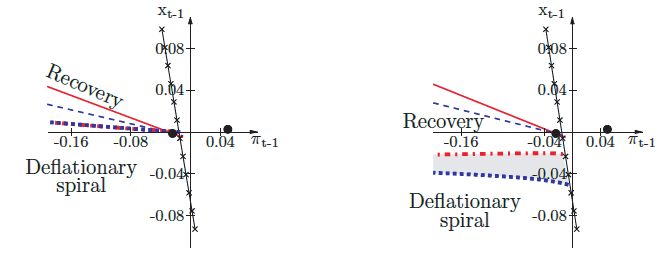
152 Journal of Economic Literature, Vol. LIX (March 2021)
of adaptively behaving people would ever hit still continuous and reversible. In the pres-
on. I think an appropriate stability theory can ence of very strong nonlinearities, multiple
be useful in weeding out these uninteresting steady states arise and catastrophic changes
equilibria … But to be useful, stability theory
must be more than simply a fancy way of saying from a “good” steady state to a “bad” or “cri-
that one does not want to think about certain sis” steady state of the system may occur after
equilibria. I prefer to view it as an experimen- small changes of parameters (e.g., Scheffer
tally testable hypothesis, as a special instance 2009, Scheffer et al. 2012). After such a cat-
of the adaptive laws that we believe govern all astrophic change, the system can not easily
human behavior.
be recovered and pushed back to the ”good”
steady state (see the caption of figure 1). Such
A key question for macroeconomic behav- strong nonlinearities can model the “dark
ior then is: what is the aggregate behavior corners” of the economy Blanchard (2014)
that a collection of adaptively behaving indi- refers to. It is very important to understand
viduals will learn to coordinate on? A second the key nonlinearities of the economy, in
key question is: how can policy affect this order to control policy parameters to prevent
complex coordination process? To discuss the system from undesirable critical transi-
these questions and survey the state of the tions and sudden collapse. Standard DSGE
art of the literature two topics are of particu- models have been criticized for not being
lar interest and deserve a brief discussion in able to predict the fi nancial-economic crisis.
this introduction: (i) complex systems and (ii) Such a critique may be unfair, because crises
macro laboratory experiments. in complex systems are very hard to predict.
There is no universal definition of a com- However, what has been more critical for the
plex system, but there are two important standard DSGE model is its almost entire
characteristics that we will stress:2 (i) nonlin- focus on (log) linearized models with fully
earity and (ii) heterogeneity. Nonlinearities rational agents and a unique equilibrium. In
can lead to multiple equilibria and, as a con- such models, by assumption, a crisis through
sequence, small changes at the micro level a critical transition can never exist. A realistic
may amplify and lead to critical transitions model of the macroeconomy should allow for
or tipping points at the macro level. Figure 1 the possibility of a crisis other than through
illustrates the phenomenon of a critical tran- large exogenous shocks.
sition—see Scheffer (2009) for an extensive A second important aspect of complex sys-
discussion. When nonlinearities are mild, a tems is that they consist of multiple (often
change in parameters only causes a gradual many) heterogeneous agents, who interact
change in the unique stable steady state of with each other. A m ulti-agent complex
the system. When nonlinearities become macro-system can not be reduced to a sin-
stronger, then a small change in parameters gle, individual agent system, but its inter-
may lead to a larger change in the stable actions at the micro level must be studied
steady state of the system, but the change is to explain its aggregate behavior.3 Complex
systems exhibit emergent macro behavior as
the aggregate outcome of micro interactions.
2 Another important aspect of complex systems that
is receiving much attention in recent work concerns net-
works. For example, financial networks may have increased
systemic risk and may have caused cascades that have exag- 3 The key observation that macro behavior in a com-
gerated the global financial-economic crisis. This aspect of plex system can not be reduced to micro behavior has
complex systems will not be dealt with here. The inter- been nicely summarized in the title of one of the first and
ested reader is, for example, referred to Iori and Mantegna seminal papers on complexity: ”More Is Different,” by
(2018) and Goyal (2018). Anderson (1972).Hommes: Behavioral and Experimental Macroeconomics and Policy Analysis 153
Panel A Panel B Panel C
F1
X↑
F2
Parameter →
Figure 1. Multiple Steady States and Critical Transitions or Tipping Points
Notes: Panel A: when nonlinearities are mild, the steady state is unique and a change in parameters only leads
to a gradual change in the stable steady state of the system. Panel B: when nonlinearities become stronger, a
small change in parameters may lead to a larger change in the stable steady state of the system, but the change
is still continuous and reversible. Panel C: with very strong nonlinearities, multiple steady states coexist and
catastrophic changes from a “good” steady state to a “bad” or “crisis” steady state of the system may occur after
small changes of a parameter. At the point F1a catastrophic change occurs and the system jumps from the
“good” upper stable steady state to the “bad” lower steady state. After such a catastrophic change, the system
can not easily be recovered as pushing back the system to the “good” steady state requires that the parameter
be decreased until the point F2, where the “bad” steady state disappears.
As a simple example from physics one may In social-economic systems a theory of indi-
think of a glass of water, exhibiting a critical vidual adaptive behavior is part of the law
transition from liquid to solid when the tem- of motion of the macroeconomy. A central
perature (which may be viewed as a “policy question to this survey is: what are the emer-
parameter”) varies and falls below 0º. In eco- gent properties of stylized complex macro-
nomics, a complex system consists of many economic systems with boundedly rational
economic agents (consumers, firms, inves- heterogeneous agents? Will a collection of
tors, banks, etc.), which may be heteroge- boundedly rational heterogeneous agents be
neous in various aspects. One would like to more likely to coordinate on the (homoge-
understand the emergent properties of com- neous) rational outcome, or are fluctuation
plex macroeconomic systems and, in particu- with booms and bust cycles a more likely
lar, how policy parameters might affect these aggregate outcome? This brings us back to
emergent aggregate outcomes. Lucas (1986) (see the earlier quote) who
Perhaps the most crucial difference from views the question of collective behavior and
complex systems in the natural sciences is coordination as an empirical question, an
that in economics and the social sciences, experimentally testable hypothesis. Indeed a
the ”particles can think” and one needs a large literature on laboratory macro exper-
theory of adaptive behavior and learning. iments has developed in recent years, in154 Journal of Economic Literature, Vol. LIX (March 2021)
articular the learning-to-forecast experi-
p rational expectations, to explain market fail-
ments to study coordination of expectations ures.5 In a recent survey Driscoll and Holden
in the lab. These macro experiments pro- (2014) summarize and discuss several con-
vide laboratory data, both at the individual cepts that behavioral economics has brought
(micro) and the aggregate (macro) level, to macro-models, such as fairness consider-
which can be used to test, falsify, calibrate, ations and other-regarding social preferences,
or even estimate behavioral models. In this cognitive biases, hyperbolic discounting of
way, behavioral theory needs laboratory test- consumption and savings, habit formation,
ing as a complementary tool for empirical and rule-of-thumb consumption. De Grauwe
analysis of various behavioral assumptions (2012), in his Lectures on Behavioral
and models. Macroeconomics, emphasizes boundedly
The survey is organized as follows. rational heterogeneous expectations in the
Section 2 discusses behavioral models with new Keynesian macro-model, where agents
different degrees of (ir)rationality. There are switch between simple forecasting heuristics
many different models with boundedly ratio- based upon their relative performance, as in
nal interacting agents. To address the “wil- Brock and Hommes (1997). There are thus
derness of bounded rationality” our focus many possible deviations—large or small—
is on parsimonious decision rules that are from the benchmark rational model. In the
validated in empirical work and laboratory traditional macroeconomic paradigm there
experiments. This leads to stylized behav- are (at least) three crucial assumptions
ioral complexity models that are still partly underlying many models: (i) agents have
analytically tractable.4 Section 3 discusses rational expectations; (ii) agents behave opti-
experimental macroeconomics and policy mally, that is, maximize utility, profits, etc.;
experiments, while section 4 summarizes and and, related to both, (iii) agents have an
discusses policy implications of the observed infinite horizon for optimization and expec-
coordination failure on n onrational, almost tations. A pragmatic (but still admittedly
self-fulfilling equilibria. subjective) definition of behavioral macro-
economics would be that (at least) one of
these assumptions is relaxed and replaced
2. Behavioral Models
by some form of bounded rationality. How
What exactly is meant by “behavioral macro- many of these assumptions should be relaxed
economics” is not easy to define. In his Nobel and by how much is then a matter of debate.
Prize lecture “Behavioral Macroeconomics For example, most a gent-based models devi-
and Macroeconomic Behavior,” Akerlof ate from all of these three assumptions, to
(2002) uses a very broad definition that, for build a completely new macroeconomic sys-
example, includes models of asymmetric tem from “bottom-up” modeling of agents’
information, maintaining the assumption of using simple micro-decision rules (heuris-
tics); see Dawid and Delli Gatti (2018) for
a recent survey on agent-based models in
4 Complementary to these stylized models, there is a macroeconomics.
large and rapidly increasing literature on a gent-based sim-
ulation models using more detailed “bottom-up” model-
ing of individual decision rules of heterogeneous agents.
The recent Handbook of Computational Economics on
heterogeneous agent modeling (Hommes and LeBaron 5 Other approaches emphasizing informational fric-
2018) provides a state-of-the-art overview; see especially tions, but maintaining rational expectation,s include
the survey by Dawid and Delli Gatti (2018) on agent-based rational inattention (Sims 2010) and imperfect knowledge
macroeconomics. (Angeletos and Lian 2016).Hommes: Behavioral and Experimental Macroeconomics and Policy Analysis 155
In our survey we focus on stylized behav- 2.1.1 Stability under Learning
ioral models with learning and heteroge-
neous expectations. The question of what For readers not familiar with adaptive
kind of (near) equilibria a population of het- learning it is useful to discuss stability under
erogeneous boundedly rational forecasters learning in a basic example. Consider a
might coordinate will play a prominent role simple linear law of motion of the economy
throughout the survey. We start the survey with an endogenous state variable x t driven
with homogeneous adaptive learning (sub- by exogenous stochastic shocks yt:
section 2.1), then move to heterogeneous
expectations (subsection 2.2) and behavioral (1) xt = a + b x et+1 + c yt−1 + ut,
new Keynesian models (subsection 2.3).
(2) yt = d + ρ yt−1 + εt.
2.1 Adaptive Learning
In the last three decades the adaptive To be concrete, one may think of xt as an
learning approach has become a standard asset price, whose evolution is affected by
model of bounded rationality in macroeco- price expectations x et+1and by an exogenous
nomics. Agents behave as econometricians AR(1) dividend process yt with autocorrela-
or statisticians and use an econometric tion parameter ρ , 0 < ρ < 1. The simplest
forecasting model—the perceived law of rational solution, called the minimum state
motion—whose parameters are updated variable (MSV) solution, is of the form
over time, for example, through recursive
ordinary least squares, as additional observa- (3) xt = α + γ yt−1 + ut,
tions become available. Early papers in this
area are, for example, by Marcet and Sargent with the price given as a linear function of
(1989a, b). The comprehensive overviews the exogenous fundamental shocks (divi-
given by Evans and Honkapohja (2001) and dends). Assume for the moment that the
more recently by Evans and Honkapohja parameters αand γ
are fixed. Given that all
(2013) have contributed much to its popu- agents believe that xt follows the perceived
larity in macroeconomics; see also Sargent law of motion (PLM) (3) the implied actual
(1993) for an early stimulating discussion of law of motion (ALM) becomes
bounded rationality and learning.
Early work stressed learning of the param- (4)xt = a + bα + bγd + (c + bγρ) yt−1 + ut.
eters of a correctly specified model, that is, a
perceived law of motion of exactly the same A rational expectations solution is then a
form as the (simplest) rational solution, with fixed point of the mapping T, from the PLM
agents learning the parameters over time. (3) to the ALM (4), and must satisfy
Such an analysis then provides a stability
theory of rational expectations equilibria and T(α, γ) = (a + bα + bγd, c + bγρ).
(5)
an equilibrium selection device to determine
which rational equilibria are stable. Stability The fixed point of the T-map corresponds to
under adaptive learning should be seen as a an REE solution and is given by:
minimum requirement of a rational expec-
tations equilibrium (REE), because without α = _
(6) a + _____________
bcd ,
stability under learning, coordination of a 1 − b ( 1 − b)( 1 − bρ)
population of adaptive agents on a rational
γ = _
c .
equilibrium seems highly unlikely. 1 − bρ156 Journal of Economic Literature, Vol. LIX (March 2021)
Adaptive learning means that agents learn the T-mapping T( α, β, γ)and simple alge-
the parameters α and γof the PLM (3) using bra yields for α and γ
the same REE fixed
estimation techniques such as ordinary least point as in (6) together with β = 0.6 It can
squares, which may be written in a recursive be shown that this REE fixed point is again
form algorithm. A simple associated E-stable. The adaptive learning process is
differential equation governs the stability of therefore robust with respect to overparam-
the adaptive learning process and is given by eterization of the PLM in (8) and the REE in
(3) is called strongly E-stable. Another par-
__
dα
bcd + (b − 1)α
= T (α, γ)− α = a + _____ simonious and perhaps plausible possibility
{__
1 − bρ
(7)
dτ 1
would be that agents believe that the PLM is
dτ = T2 (α, γ)− γ = c + (bρ − 1)γ.
dγ
of the simpler form
The REE in (3) is also a fixed point of this (9) xt = α + β xt−1 + ut,
differential equation (7) and, in this example,
it is a (locally) stable fixed point, when the that is, agents do not realize that xt is
parameters bρ < 1. One of the main gen- driven by an exogenous fundamental pro-
eral results form the adaptive learning liter- cess yt, but simply forecast xt by lagged
ature is the E-stability principle stating that observations xt−1. This is a simple exam-
an REE (i.e., a fixed point of the T -map) is ple of misspecification, where the PLM is
locally stable under adaptive learning pro- different from the MSV solution. We will
cesses such as ordinary least squares (OLS), return to the important issue of misspecifi-
when it is a locally stable fixed point of the cation in subsection 2.1.3.
associated ordinary differential equation
2.1.2 Endogenous Fluctuations under
(ODE). In this particular example, when
Adaptive Learning
agents believe that the PLM is of the form
(3) and learn the parameters through OLS, Early work stressed adaptive learning as
the learning process converges (locally) to an equilibrium selection device of REE and
the REE. E -stability should be viewed as a studied E -stability of rational equilibria in
necessary condition for REE to be empiri- various models, for example, in an asset pric-
cally relevant. If an REE is not E-stable, ing model with informed and uninformed
then coordination of a large population of traders (Bray 1982), the cobweb model
adaptive agents on such an equilibrium (Bray and Savin 1986), in a general class of
seems highly unlikely. linear stochastic models (Marcet and Sargent
But what happens if the agents believe in 1989b) and in linear models with private
a different PLM than the MSV solution (3)? information (Marcet and Sargent 1989a).
For example, to forecast the state vari- Later work has shown that adaptive learn-
able xtit seems natural to include its lagged ing need not converge to a rational expecta-
value xt−1. Assume that instead of (3), agents tions equilibrium, but learning may induce
believe that the PLM is of the (slightly) more endogenous (periodic or even chaotic) busi-
general form ness cycle fluctuations. Examples include
the learning equilibria in overlapping gen-
(8) xt = α + β xt−1 + γ yt−1 + ut. erations models (Bullard 1994; Grandmont
This is an example where the PLM is overpa- 6 There is an additional REE fixed point β = 1 /b,
rameterized with respect to the MSV ratio- representing rational bubble solutions; see Evans and
nal solution. In a similar way one can extend Honkapohja (2001).Hommes: Behavioral and Experimental Macroeconomics and Policy Analysis 157
1985, 1998), learning to believe in chaos Agents can choose between a risk-free
(Schönhofer 1999), the consistent expecta- asset paying a fixed return rand a risky asset
tions equilibria in nonlinear cobweb models (say a stock) paying stochastic dividends.
(Hommes and Sorger 1998), the learning to Denote ytas the dividend payoff and p t as
believe in sunspots (Woodford 1990), and the asset price. Agents are risk averse and
the exuberance equilibria (Bullard, Evans, assumed to be myopic mean-variance maxi-
and Honkapohja 2008). mizers. The mean-variance demand zdt is
Constant Gain Learning.—Adaptive + yt+1) − (1 + r) pt
E ⁎t (pt+1
learning typically generates slow learning (10) zdt =
_____________________
aσ 2t
of parameters, because standard recursive
estimation algorithms give equal weight
to all past observations. Consequently, the + yt+1)denotes the condi-
where E ⁎t (pt+1
weight given to the most recent observa- tional expectation of p t+1 + yt+1, a is the risk
tion becomes smaller and converges to 0 as aversion, and σ 2t denotes agents’ conditional
the number of observations goes to infin- expectations about the variance of excess
ity. The vanishing weight given to the most returns pt+1 + yt+1 − (1 + r) pt. The equi-
recent observation typically has a stabilizing librium price is derived from market clear-
effect on the learning dynamics. An alterna- ing zdt = zst and given by
tive parameter updating scheme is constant
1 + r [ t ( t+1 t st]
gain learning, giving a fixed weight (the gain
(11) pt = _ 1 E ⁎ p + y − aσ 2 z .
t+1)
coefficient) to the most recent observations.
Constant gain learning is consistent with lab
experiments and survey data, where subjects The term a σ t2 zst may be seen as a t ime-varying
or forecasters typically give more weight risk premium. Dividends y tand the supply of
to the most recent observations. Constant shares zstare assumed to follow simple inde-
gain learning models often give a better fit pendent and identically distributed (IID)
to macro and financial data and are able stochastic processes. Assuming σ 2t = σ 2 at
to generate observed stylized facts in time steady state, the rational fundamental price
series data, such as high persistence, excess can be computed as the discounted sum of
volatility, and clustered volatility (Evans and future dividends minus the time-varying risk
Honkapohja 2001; Sargent 1993; Milani premium, and is given by
2007, 2011; Branch and Evans 2010). ∞ ∞
p ⁎t = ∑ β jEt(yt+j) − β ∑ β jaσ 2 Et(zst+j
),
Bubbles and Crash Dynamics under j=1 j=0
Learning.—Branch and Evans (2011a) where β = 1 / (1 + r)is the discount fac-
develop a simple linear m ean-variance asset tor. There is additionally a class of rational
pricing model capable of generating bubbles
and crashes when agents use constant-gain
learning to forecast expected returns and the whose properties are in line with historical bubble epi-
conditional variance of stock returns.7 sodes. West (1987), Froot and Obstfeld (1991), and Evans
(1991) construct rational bubbles that periodically explode
and collapse. A controversial issue for rational bubbles is
that the trigger for the bubble collapse is often modeled
7 There is a large literature on periodically collapsing by an exogenous sunspot process. In the model of Branch
rational bubbles. Blanchard and Watson (1982) develop and Evans (2011a) bubbles and crashes arise endogenously
a theory of rational bubbles in which agents’ (rational) as self-fulfilling responses to fundamental shocks, arising
expectations are influenced by extrinsic random variables from the adaptive learning of agents.158 Journal of Economic Literature, Vol. LIX (March 2021)
ubble solutions, which are given by adding
b substantial excess volatility. In this regime,
to the fundamental solution a rational bub- revisions of risk estimates play an important
ble term β
−t ηt, where ηtis an arbitrary mar- role in generating the movements of prices
tingale, i.e., Et ηt+1
= ηt. Since 0 < β < 1 that sustain the random walk beliefs. In sum-
the rational bubbles are explosive. Branch mary, risk in an adaptive learning with con-
and Evans (2011a) show that the fundamen- stant gain setting plays a key role in triggering
tal solution is E -stable under learning, while asset price bubbles and crashes. These intu-
the rational bubble solutions are unstable itive and plausible results provide insights
under learning. into the mechanisms by which expectations,
In Branch and Evans (2011a) agents’ per- learning, and bounded rationality generate
ceived law of motion is of the simple linear large swings in asset prices.
AR(1) form
2.1.3 Misspecification Equilibria
(12) pt = k + c pt−1 + ϵt, Under adaptive learning the PLM will, in
general, be misspecified, that is, the PLM
where ϵtis an IID noise term. This linear is generally different from the ALM. This
specification coincides with the general form observation has lead to the study of misspeci-
of the rational bubble solutions. Adaptive fication equilibria under learning (Evans and
learning then consists of a recursive ordi- Honkapohja 2001, Sargent 1999, Branch and
nary least squares updating scheme for the McGough 2005, see especially the stimulat-
two parameters k and cof the conditional ing survey in Branch 2006). The idea here
mean forecast together with a recursive is that the representative agent uses a sim-
algorithm for the conditional variance σ 2t of ple, parsimonious PLM to learn about the
excess returns. For both learning processes unknown ALM of the economy. These sim-
constant gains can be used. Recursive updat- ple learning equilibria may be a more plau-
ing of both the conditional variance and sible outcome of the learning process of a
the expected return implies several mecha- population of adaptive agents.
nisms through which learning impacts stock Different types of parsimonious misspeci-
prices. Extended periods of excess volatility, fication equilibria have been proposed in the
bubbles, and crashes arise with a frequency literature. An interesting class are the natural
that depends on the extent to which past expectations (Fuster, Laibson, and Mendel
data is discounted. A central role is played 2010; Fuster et al. 2012; and Beshears et al.
by changes over time in agents’ estimates of 2013), where agents use a simple parsimoni-
risk. First, occasional shocks can lead agents ous fixed (higher order) AR(p) rule in fore-
to revise their estimates of risk in a dramatic casting to explain the long-run persistence
fashion. A sudden decrease or increase in the of economic shocks. Since the parameters
estimated risk of stocks can propel the sys- are fixed, strictly speaking this does not fall
tem away from the fundamental equilibrium under adaptive learning, but its parsimony
and into a bubble or crash. Second, along an makes natural expectations intuitive and
explosive bubble path, risk estimates tend to plausible forecasting rules.
increase and can become high enough to lead Branch (2006) considers adaptive learn-
asset demand to collapse and stock prices ing where the PLM is underparametrized,
to crash. Third, under learning, estimates because agents do not take all relevant exog-
for stock returns will occasionally escape to enous shock processes into account in their
random walk beliefs that can be viewed as a PLM. These beliefs, however, satisfy a least
bubble regime in which stock prices exhibit squares orthogonality condition consistentHommes: Behavioral and Experimental Macroeconomics and Policy Analysis 159
with John Muth’s original hypothesis. The their relative performance, as in Brock and
least squares orthogonality condition in Hommes (1997). The model exhibits multi-
these models imposes that beliefs gener- ple misspecification equilibria (ME) and the
ate forecast errors that are orthogonal to an real-time learning dynamics switch between
agent’s forecasting model; that is, there is no these different equilibria mimicking clus-
discernible correlation between these fore- tered volatility in asset returns.
cast errors and an agent’s model. Under this Branch and Evans (2011b) use a similar
interpretation, the orthogonality c ondition approach in a new Keynesian macro model
guarantees that agents perceive their beliefs and study monetary policy under learning.
as consistent with the real world. Thus, There are two types of exogenous shocks to
agents can have misspecified (i.e., not ratio- the economy: cost push shocks to the new
nal expectations (RE)) beliefs, but within Keynesian Phillips curve (NKPC) and supply
the context of their forecasting model they shocks to the investment–savings (IS) curve,
are unable to detect their misspecification. both following exogenous stochastic AR(1)
An equilibrium between optimally misspec- processes. The RE MSV solution of the
ified beliefs and the stochastic process for economy is a linear function of both shocks.
the economy is called a restricted percep- There are two types of agents in the econ-
tions equilibrium (RPE). omy, one type using forecasts based only on
Branch and Evans (2010) apply these the demand shocks and a second type using
ideas in a m ean-variance asset pricing forecasts based only on the supply shocks.
model, where both dividends and the supply Branch and Evans (2011b) demonstrate that,
of shares follow exogenous stochastic AR(1) even when monetary policy rules satisfy the
processes. There are two types of agents, Taylor principle by adjusting nominal inter-
who have different types of misspecified est rates more than one for one with infla-
underparametrized price forecasting mod- tion, there may exist equilibria with intrinsic
els. One type has a price forecasting model heterogeneity, where the two types of agents
only based on the AR(1) dividend process, coexist. Under certain conditions, there may
while the other type forecasts prices only exist multiple misspecification equilibria.
based on the AR(1) process for the supply These findings have important implications
of shares. The RPE requires that agents for business cycle dynamics and for the
forecast in a statistically optimal manner. It design of monetary policy. Branch and Evans
is required that the forecast model param- (2011b) then study the role that policy plays
eters are optimal linear projections, that is, in determining the number and nature of
the belief parameters, satisfy least-squares misspecification equilibria.
orthogonality conditions. Within the con-
2.1.4 Behavioral Learning Equilibria
text of their forecasting model, agents are
unable to detect their misspecification. Of The most crucial aspect of adaptive learn-
course, if they step out of their model and ing is probably the choice of the PLM. For
run specification tests, they could detect a large population of adaptive agents being
the misspecification. But real-time simula- able to coordinate their beliefs, the parsi-
tions show that the misspecification is hard mony of the PLM seems crucial. Hommes
to detect and, for finite time, agents may not and Zhu (2014) introduced a particularly
be able to reject their underparameterized simple form of misspecification called
models. They then study a misspecification behavioral learning equilibrium. The idea
equilbrium with intrinsic heterogeneity, and here is that for each variable to be fore-
fractions of the two types of agents based on casted in the economy agents use a simple160 Journal of Economic Literature, Vol. LIX (March 2021)
(misspecified) univariate AR(1) forecast- where πtis the inflation at time t, π et+1 is the
ing rule. A behavioral learning equilibrium subjective expected inflation at date t + 1,
(BLE) arises when the sample average and ytis the output gap or real marginal cost,
the first-order autocorrelations of the AR(1) δ ∈ [0, 1)is the representative agent’s sub-
rule coincide with the observed realiza- jective time discount factor, γ > 0is related
tions. Hence, along a BLE the parameters to the degree of price stickiness in the econ-
of the AR(1) rule are not free, but pinned omy, and ρ ∈ [0, 1)describes the persistence
down by two simple observable statistics, the of the AR(1) driving process. Variables u t
sample average and the fi rst-order sample and εtare IID stochastic disturbances with
autocorrelation.8 Agents thus use the optimal zero mean and finite absolute moments with
AR(1) forecasting heuristics. Such a simple, variances σ 2u and σ 2ε , respectively.
parsimonious learning equilibrium may be a Under RE inflation πtis a linear function
more plausible outcome of the coordination of the fundamental driving process y t. The
process of individual expectations in large REE therefore has the same persistence and
complex socioeconomic systems. The use autocorrelations as the fundamental shocks.
of simple low-order autoregressive rules to Assume instead that agents are boundedly
forecast has also been documented in labora- rational and do not recognize or do not
tory experiments with human subjects (e.g., believe that inflation is driven by output gap
Assenza et al. 2014). or marginal costs, and therefore do not rec-
Hommes and Zhu (2014) apply the BLE ognize that inflation should be a linear func-
concept in the simplest class of models, tion of the exogenous shocks. Rather, agents
where the actual law of motion of the econ- believe that inflation follows a stochastic
omy is a one-dimensional linear stochastic AR(1) process and simply forecast inflation
process driven by exogenous AR(1) shocks.9 by a ( two-period ahead) univariate AR(1)
Two important applications of this frame- rule, i.e., π et+1 = α + β 2( πt−1
− α). The
work are an asset pricing model driven by implied ALM then becomes
AR(1) dividends and an NKPC with infla-
{yt = a + ρ yt−1+ εt.
tion driven by an AR(1) process for marginal πt = δ[ α + β 2( πt−1
− α)] + γ yt+ ut,
costs. (14)
The NKPC with inflation driven by an
exogenous AR(1) process yt is given by
(Woodford 2003) Hommes and Zhu (2014) compute the cor-
responding fi rst-order autocorrelation coef-
πt = δπ et+1 + γ yt + ut,
{yt = a + ρ yt−1 + εt,
ficient F( β)of the implied ALM (14) as
(13)
F(β)
(15)
γ 2ρ( 1 − δ 2 β 4)
= δβ 2 + __________________________
σ 2
.
8 The idea behind BLE originates from the consistent γ 2(δβ 2 ρ + 1) + (1 − ρ 2)(1 − δβ 2ρ) ⋅ _u2
σ ε
expectations equilbria in Hommes and Sorger (1998),
where the beliefs about sample average and all autocor-
relations β k, for all lags k , coincide with the realizations.
and show that there exists at least one non-
Lansing (2009, 2010), applies the idea of (first-order) con- zero BLE (α ⁎, β ⁎) with α ⁎ = ¯
π ⁎ (i.e., the
sistent expectations in a new Keynesian framework. sample average equals REE inflation) and β ⁎
a fixed point of the autocorrelation map F(β)
9 Hommes et al. (2019) recently extended the BLE con-
cept to higher dimensional linear stochastic models and
estimated BLE in the Smets–Wouters DSGE model. in (15).Hommes: Behavioral and Experimental Macroeconomics and Policy Analysis 161
Hommes and Zhu (2014) also show that ersistence. For initial states close to the tar-
p
when F′ (β ⁎) < 1the E-stability principle get, SAC learning converges to the low per-
holds for the sample autocorrelation (SAC) sistence BLE. For initial states further away
learning process to learn the optimal param- from the target, SAC learning converges
eters α ⁎ and β ⁎. The time-varying parame- to the high-persistence BLE. Under con-
ters are given by the sample average stant gain learning, the system may switch
between both BLE. These results are con-
t sistent with the empirical finding in Adam
(16) αt = _ 1 ∑ x, (2007) that the restricted perception equi-
t + 1 i=0 i
librium (RPE) describes subjects’ inflation
rst-order SAC coefficient10
and the fi expectations surprisingly well and provides
a better explanation for the observed per-
∑t−1
i=0 (xi − αt) ( xi+1 − αt) sistence of inflation than REE. Multiplicity
(17) βt = _____________________
.
∑ti=0( xi − αt) 2 of learning equilibria leaves an important
task for monetary policy to keep inflation
Interestingly, for the NKPC multiple BLE and output in the low-volatility regime. This
may coexist, because the nonlinear autocor- simple model also shows how a simple and
relation map F( β)may have multiple fixed plausible form of misspecification brings us
points. Figure 2 illustrates the coexistence from a perfect rational world with a unique
of a low- and a high-persistence BLE, equilibrium into a more realistic complex
which are both stable under SAC learning boundedly rational reality with multiple
for appropriate initial states. The low-per- equilbria and critical transitions.
sistence regime represents a rather stable
2.1.5 Policy under Adaptive Learning
economy with inflation close to target, while
the high-persistence regime is rather unsta- If coordination of a population of agents is
ble with long-lasting periods of high or low better described by an adaptive learning pro-
inflation. The high-persistence BLE is char- cess than by a rational expectations equilib-
acterized by β ⁎ ≈ 0.996, very close to unit rium, this has important policy implications.
root, and thus exhibits persistence amplifi- This subsection discusses some examples
cation, with much more persistence in infla- of policy analysis under models of adaptive
tion then under RE. Under SAC learning learning.
with constant gain, the economy may switch In rational expectations models one can
irregularly between phases of low and high distinguish between determinacy and inde-
persistence and volatility in inflation. terminacy of equilibria. An REE is deter-
This example shows how a very simple minate when there exists a unique solution,
form of misspecification may lead to mul- typically a saddle-path solution converging
tiple equilibria and tipping points or crit- to the rational steady state. An REE is inde-
ical transitions (compare figure 1 in the terminate when multiple (typically a contin-
introduction to figure 2, panel H) between uum) of solutions converging to the steady
different regimes of low volatility and state exist. In such a case, often additional
low persistence to high volatility and high sunspot equilibria exist. If an REE is deter-
minate, it is usually assumed that agents
coordinate on the unique s addle-path solu-
10 An important and convenient feature of this nat-
tion. Such a saddle-path solution usually
ural learning process is that −
1 ≤ βt ≤ 1, since it is a
(
first-order) autocorrelation coefficient (Hommes and can only be computed by advanced compu-
Sorger 1998). tational software, such as the widely used162 Journal of Economic Literature, Vol. LIX (March 2021)
Panel A. Low persistence BLE Panel B. Sample average α t Panel C. Sample auto correlation β t
0.05 0.034 1
0.045
0.04 0.032
0.035
0.03
πt
αt
βt
0.03 0.5
0.025
0.02 0.028
0.015
0.01 0.026 0
00
0
50
0
0
0
0
0
0
0
0
0
0
0
0
0
0
0
0
0
0
10
15
20
25
30
35
00
00
00
00
50
00
50
00
50
00
,0
2,
4,
6,
8,
1,
1,
2,
2,
3,
10
t t t
Panel D. High persistence BLE Panel E. Sample average α t Panel F. Sample auto correlation β t
0.16 0.13 1
0.14 0.12
0.12
0.1 0.11
πt
αt
βt
0.08 0.1 0.5
0.06 0.09
0.04
0.08
0.02
0 0
0
50
0
0
0
0
0
0
0
5
1
5
2
0
5
1
5
2
10
15
20
25
30
35
0.
1.
0.
1.
t t ×104 t ×104
Inflation at SCEE Inflation at REE
Panel G Panel H
1 1.5
0.8
1 1-order autocorrelation of REE
0.6 High stable β*
F(β)
β*
0.4 Low stable β*
0.5 Middle unstable β*
0.2
0 0
0
2
4
6
8
1
7
75
8
85
9
95
1
0.
0.
0.
0.
0.
0.
0.
0.
0.
0.
β ρ
Figure 2. Multiple Behavioral Learning Equilibria in the NK Model
Notes: Top panels: convergence of SAC learning to low-persistence BLE (α ⁎, β ⁎1) = (0.03, 0.3066). Middle
panels: convergence to high-persistence BLE (α ⁎, β ⁎3) = (0.03, 0.9961) exhibiting persistence amplification
(for REE autocorrelation is ρ = 0.9). Panel G: BLE β ⁎correspond to the three fixed points of autocorrelation
map F(β) in (15). Panel H: BLE as a function of autocorrelation parameter ρ of the shocks; more persistent
shocks lead to critical transition to persistence amplification (Hommes and Zhu 2014).
Dynare software, assuming that the equa- edge of the law of motion of the economy,
tions of the economy are common knowl- is however lacking, and without an adaptive
edge. A learning theory of coordination learning process, coordination of a popula-
on a saddle-path equilibrium, without the tion of individuals on an equilibrium, even
demanding assumption of perfect knowl- if it is unique, seems unlikely.Hommes: Behavioral and Experimental Macroeconomics and Policy Analysis 163
Bullard and Mitra (2002) study mone- where the coefficients ϕ π, ϕx > 0 determine
tary policy under adaptive learning of the how strongly the central bank (CB) responds
MSV solution in the new Keyensian model to inflation and output gap respectively.
and show that considering learning gener- Bullard and Mitra (2002) show that for
ally can alter the evaluation of alternative the contemporaneous interest rate rule the
policy rules. The (log-linearized) NK model determinacy (indeterminacy) region under
is given by Clarida, Galí, and Gertler (1999) RE coincides exactly with the E -stability
and Woodford (2003) (E-instability) region under learning. In
this case, the policy analysis under RE and
(18) xt = Ẽ t xt+1 + _
1 ̃ − i + u,
σ (E t πt+1 t) t adaptive learning of the MSV solution are
the same. For the forward-looking and the
(19) πt = κ xt + δ Ẽ t πt+1
+ vt, backward-looking Taylor rules, however,
these regions do not coincide, and determi-
where xtis the output gap, πt inflation, nacy under RE does not imply E-stability
i t the nominal interest rate, Ẽ t xt+1, Ẽ t πt+1
under learning. This stresses the fact that
are expectations about next period’s output policy should be based on plausible and
gap and inflation, and ut and vt are exogenous empirically relevant models of adaptive
shocks following AR(1) processes. Equations learning. For all policy rules the Taylor prin-
(18) and (19) represent the IS curve and the ciple holds under learning, that is, adjust-
Phillips curve. Here δ is the discount factor, ing the nominal interest rates more than
and one-for-one in response to inflation above
target implies learnability. In subsection 3.2
(σ + η)( 1 − ω)( 1 − δω) we will return to this issue and discuss some
κ =
(20) ____________________
ω ,
laboratory experiments to test the validity
of the Taylor principle. Bullard and Mitra
with σand ηthe inverses of, respectively, the (2002) stress the general point that learn-
elasticity of intertemporal substitution and ability should be a necessary additional cri-
the elasticity of labor supply, and (1 − ω) is terion for evaluating alternative monetary
the fraction of firms that can adjust their price policy rules.
in a given period. Expectation Ẽ t follows an
adaptive learning process of the MSV solution Monetary and Fiscal Policy in a Non-
yt = a + byt−1 + c wt, where yt = [xt, πt] T
linear NK Model.—Evans, Guse, and
and wt = [ut, vt] T. Honkapohja (2008) and Benhabib, Evans,
The nominal interest rate is set by the and Honkapohja (2014) study the a non-
central bank and Bullard and Mitra (2002) linear NK model with a zero lower bound
consider three different specifications of the (ZLB) on the interest rate under adaptive
Taylor interest rate rule, where the interest learning of the steady state. In this nonlinear
rate is set in response to deviation of inflation NK model, two steady states may coexist, the
and output gap from the targets: target steady state and a ZLB steady state,
and liquidity traps or deflationary spirals may
(21) it= ϕπ πt+ ϕx xt (contemporaneous)arise. The nonlinear equations describing
aggregate dynamics are given by
(22) it= ϕπ πt−1
+ ϕx xt−1 (lagged)
π e
( β Rt )
1/σ
t+1
(24) ct = c et+1 _ ,
(23) it= ϕπ Ẽ tπt+1
+ ϕx Ẽ txt+1 (forward looking)164 Journal of Economic Literature, Vol. LIX (March 2021)
(25) πt(πt − 1) = β π et+1( π et+1 − 1) rule (26) is defined as aggressive since, while
in “normal” times (πt ≥ π̃ ) it follows a stan-
υ
+ _
αγ (ct + gt)
1+ϵ
_
α
dard forward-looking Taylor rule, it pre-
ventively cuts the nominal interest rate to
1 − υ c + g c −σ
+ _ γ ( t t) t , the ZLB each time inflation drops below a
given threshold π̃ . The reaction coefficients
in the interest rate rule are set to ϕπ = 2
⎧
⎪
and ϕy = 0.5, which are in line with empir-
ϕ R ⁎ ϕ R ⁎
π e
1 + R − 1 (_ ⁎ ) ( ⁎)
_ _ y
⁎ πe R ⁎−1 _ ct+1 R ⁎−1
( )
t+1
π
c ical estimates. This parametrization ensures
Rt = ⎨ if πt ≥ π ̃
⎪R̃
(26) local determinacy of the targeted steady state
(π ⁎, c ⁎) under RE. However, as emphasised
⎩ if πt < π̃ . by Benhabib, Schmitt-Grohé, and Uribe
(2002), “active” Taylor rules imply the exis-
tence of a second low-inflation steady state
Equation (24) describes the dynamics of net (πL , cL ) , which is locally indeterminate under
output ct(i.e., output minus government RE.
spending) through a standard Euler equa- Fiscal policy is specified as
tion, where c et+1 and π et+1 denote respectively
expectations of future net output and infla- (27) gt = g¯ ,
tion, Rtis the nominal gross interest set by
the central bank, 0 < β < 1is the discount where g¯ is fixed. Evans, Guse, and Honkapohja
factor, and σ > 0refers to the intertempo- (2008) set π ⁎ = 1.05which implies a net out-
ral elasticity of substitution. put steady state value of c ⁎ = 0.7454. Under
Equation (25) is an NKPC describ- the aggressive monetary policy in equa-
ing the dynamics of inflation πt, tion (26), the l ow-inflation steady state is given
where gtis government spending of the aggre- by (πL , cL ) = (0.99, 0.7428). The two equi-
gate good, ϵ > 0refers to the marginal libria of the model are depicted in figure 3.
disutility of labor, 0 < α < 1is the return Evans, Guse, and Honkapohja (2008) con-
of labor in the production function, γ > 0 sider a fiscal switching rule that can prevent
is the cost of deviating from the inflation liquidity traps and deflationary spirals. The
target under Rotemberg price adjustment fiscal switching rule prescribes an increase in
costs, and υ > 1is the elasticity of substi- public expenditures g t each time monetary
tution between differentiated goods. The policy fails to achieve πt > π̃ . In model (24)–
term πt( πt − 1)in equation (25) arises from (25), given expectations π et+1 and c et+1, any
the quadratic form of the adjustment costs. level of inflation π tcan be achieved by set-
Let Qt ≡ πt( πt − 1). The appropriate root ting gtsufficiently high. The idea behind the
for given Qis π ≥ 1/ 2, so one needs to monetary–fiscal policy mix is the following.
impose Q ≥ − 1 /4to have a meaningful If the inflation target is not achieved under a
definition of inflation. standard Taylor rule, monetary policy is first
Equation (26) describes an aggressive relaxed in order to stimulate the economy.
monetary policy, where R̃ = 1.0001 corre- If the ZLB constraints the effectiveness of
sponds to the ZLB on the nominal interest monetary policy, aggressive fiscal policy is
rate.11 The forward-looking monetary policy then activated. As shown by Evans, Guse, and
Honkapohja (2008), setting π L You can also read


