Industrial clusters in the long run: Evidence from Million-Rouble plants in China

Industrial clusters in the long run:
      Evidence from Million-Rouble plants in China∗
           Stephan Heblich               Marlon Seror                  Hao Xu
                                   Yanos Zylberberg
                                  December 18, 2020

                                         Abstract

          We identify the negative spillovers exerted by large, successful factories on
      other local production units in China. A short-lived cooperation program be-
      tween the U.S.S.R. and China led to the construction of 156 “Million-Rouble
      plants” in the 1950s. The identification exploits the ephemeral geopolitical
      context and exogenous variation in location decisions due to the relative po-
      sition of allied and enemy airbases. We find a rise-and-fall pattern in counties
      hosting a factory and show that (over-) specialization explains their long-run
      decline. The analysis of production linkages shows that a large cluster of
      non-innovative establishments enjoy technological rents along the production
      chain of Million-Rouble plants. This industrial concentration reduces the local
      supply of entrepreneurs.

          JEL codes: R11, R53, J24, N95

  ∗
    Heblich: University of Toronto, CESifo, IfW Kiel, IZA, SERC; stephan.heblich@utoronto.ca;
Seror: University of Bristol, Paris School of Economics, DIAL, marlon.seror@bristol.ac.uk;
Xu: China Construction Bank, sysxuhao@163.com; Zylberberg: University of Bristol, CESifo,
Alan Turing Institute; yanos.zylberberg@bristol.ac.uk. This work was part-funded by the Eco-
nomic and Social Research Council (ESRC) through the Applied Quantitative Methods Network:
Phase II, grant number ES/K006460/1, and a BA/Leverhulme Small Research Grant, Reference
SRG\171331. We are grateful to Sam Asher, Kristian Behrens, Sylvie Démurger, Christian Dust-
mann, James Fenske, Richard Freeman, Jason Garred, Ed Glaeser, Flore Gubert, Marc Gurgand,
Ruixue Jia, Vernon Henderson, Matthew Kahn, Sylvie Lambert, Florian Mayneris, Alice Mes-
nard, Thomas Piketty, Simon Quinn, Steve Redding, Arthur Silve, Uta Schönberg, Jon Temple,
and Liam Wren-Lewis for very useful discussions. We also thank participants at Bristol, CREST,
DIAL, Geneva, Georgia Tech, Goettingen, Laval (Quebec), LSE, Ottawa, Oxford, PSE, Toronto,
UCL, UQAM, the EUEA 2018 (Düsseldorf), EEA 2018 (Cologne), UEA 2018 (New York), IOSE
2019 (St Petersburg), EHES 2019 (Paris), Bath, CURE 2019 (LSE), Cities & Development 2020
(Harvard) for helpful comments. We thank Liang Bai, Matthew Turner, Andrew Walder, and Siqi
Zheng for sharing data. The usual disclaimer applies.

The structural transformation of agrarian economies involves high spatial con-
centration of economic activity (Kim, 1995; Henderson et al., 2001). Regions that
attract industrial clusters during this transformation process typically experience a
boom followed by a bust, as illustrated by declining factory towns in the United
States (Detroit and the “Rust Belt”), the United Kingdom (Manchester and other
cotton towns), the Ruhr region in Germany, or the Northeast of France. Explana-
tions for such a decline usually rely on external, aggregate factors: (i) structural
change, as employment shifts away from industry and into services (Ngai and Pis-
sarides, 2007; Desmet and Rossi-Hansberg, 2014), or (ii) exposure to international
competition (Pierce and Schott, 2016).
    This paper presents causal evidence of a boom and a bust following successful
industrial investments, without any external factor triggering a downturn. This
allows us to focus on factors within the local economy that drive the bust. The local
economy is unproductive, non-innovative, and very specialized. In order to shed
light on the relationship between industrial concentration and firm performance, we
exploit high-quality data on production, patent applications and possible linkages
between manufacturing establishments (1992–2008). We find that the local economy
is characterized by a hub and spoke structure where one large, successful industrial
plant is linked to a network of rent-extracting firms along its production chain. This
structure limits technological spillovers across industries and leads to the migration
of entrepreneurs to other Chinese cities.
    We exploit an unprecedented investment and technology transfer from the U.S.S.R.
to China, which led to the construction of 156 “Million-Rouble Plants” (MRPs)
between 1953–1958. These plants, equipped with advanced Soviet technology, con-
stitute the foundation stone of China’s industrialization (Lardy, 1987; Naughton,
2007). Identifying industrial spillovers requires exogenous variation in the initial
distribution of these large industrial units. In an ideal setting, actual project sites
would have a natural set of counterfactual industry locations, e.g., a list of candidate
locations as in Greenstone et al. (2010), and an exogenous component in the selec-
tion process among these locations. We emulate this hypothetical setup as follows.
We first rely on the historical site-selection criteria described in Bo (1991) to select
a set of suitable counties based on economic factors (e.g., market access and access
to natural resources) which were carefully considered by planners.1 We then exploit
   1
     In stark contrast with the Great Leap Forward or the Third Front Movement (whose invest-
ments had to be “close to the mountains, dispersed, and hidden in caves”), this program was effi-
ciently implemented. The choice of locations for these plants was economically sound and spanned
a wide range of locations in China; great attention was also given to production efficiency, including
material incentives for managers (Eckstein, 1977; Selden and Eggleston, 1979) and technological
transfers (as documented by Giorcelli, 2019, for the Marshall plan).

                                                  2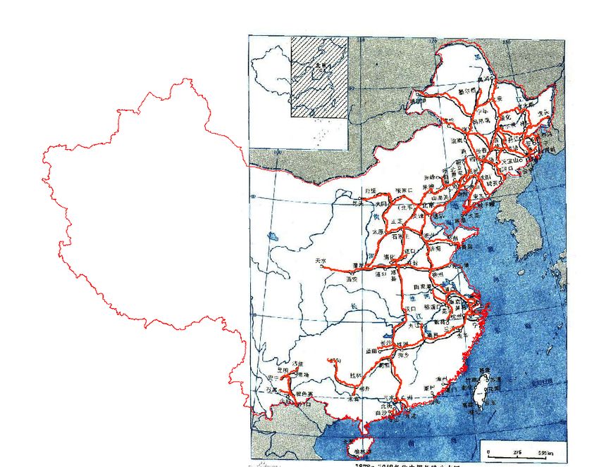

the ephemeral geopolitical context—the short-lived Sino-Soviet Treaty of Friend-
ship, Alliance and Mutual Assistance—to isolate temporary, exogenous variation in
the probability to host a large factory for suitable counties. After the Korean war,
Chinese planners were wary of the new factories’ vulnerability to enemy bombing;
this had a marked effect on the location of MRPs.2 We model the bombing threat
by combining detailed information about airplane technologies with the location of
enemy and allied air bases, and we instrument the probability to host a MRP by the
vulnerability to air strikes from major U.S. bases as computed between 1950–1960,
controlling for vulnerability after the Sino-Soviet split.3 The instrument may still
correlate with other geographic factors playing a role during the recent economic
growth. We show that our findings are robust to controlling for: (i) current market
access, distances to major (exporting) ports, to the Pearl River Delta, and to the
coast; (ii) amenities and unfavorable geographic characteristics (e.g., ruggedness);
(iii) other spatial policies, e.g., Special Economic Zones (see, e.g., Wang, 2013) or
the Third Front Movement (Fan and Zou, 2019).
     We show that counties hosting MRPs experience a rise-and-fall pattern. In 1982,
treated counties were more industrialized and two to three times more productive
than control counties.4 However, these treated counties experienced a steady decline
(in relative terms) over the following decades, even though the MRPs themselves
remained very productive.5 In 2010, the employment share in industry was lower in
treated counties, and there was no longer any difference in average productivity. We
then characterize production in the average (other) manufacturing establishment:
within a given industry, the non-MRPs establishments in treated counties pay lower
wages in spite of a more educated workforce, are less productive, less innovative,
and less competitive than establishments in control counties.
     To assess whether and how MRPs exert negative spillovers on other production
units, we rely on a procedure developed in Imbert et al. (2020) which associates a
    2
      Senior generals were directly involved in siting decisions to protect the state-of-the-art factories
from enemy airstrikes, using intelligence maps of the U.S. and Taiwanese air bases (Bo, 1991).
Historical U.S.S.R. documents report the same strategy to locate Soviet Science Cities out of the
reach of enemy bombers (Schweiger et al., 2018).
    3
      The set of protected locations then became smaller, which called for directing new industrial
investments to the interior in a policy called the Third Front Movement (see Fan and Zou, 2019).
    4
      The research requires high-quality data on economic activity at the county level (about 2,400 in
China). Aggregate data are available from the early stages of industrialization, with the 1953, 1964,
1982, 1990, 2000, and 2010 Censuses. In the recent period, we rely on a census of manufacturing
firms, the National Bureau of Statistics “above-scale” annual establishment survey (1992–2008),
which we link with patent applications (He et al., 2018) and complement with measures of factor
productivity (Imbert et al., 2020) and markups (following De Loecker and Warzynski, 2012).
    5
      We identify the MRPs in a census of manufacturing establishments and find that they are still
outliers in terms of productivity and innovation—without any signs of decline.

                                                    3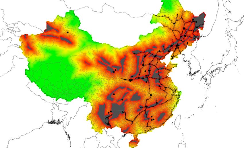

unique HS6 product code to textual product descriptions provided by manufacturing
establishments. We use this product classification to construct Herfindahl indices of
product concentration, mitigated by input/output linkages or technological linkages
(Bloom et al., 2013), and evaluate the role of (over-)specialization in explaining
firm performance in treated counties. We find that treated counties are highly
concentrated in production. As counties with a specialized production structure
are less productive, this shift in specialization induces a drop in firm performance.
We then look at the role of production linkages at a more granular level, and we
show that treated counties are highly concentrated along the production chain of the
MRPs. The large cluster of linked establishments, upstream and downstream of the
MRP(s), is quite productive but not innovative—registering almost no patents—and
not competitive—charging a higher mark-up. These establishments, by operating
along the production chain of a large and productive factory, tie their production
to the larger factory, enjoy a technological rent by doing so, and are not incited
to incur innovation efforts. Treated counties do not benefit from between-industry
technological spillovers, which have been identified as the drivers of innovation and
development in the long run (see Carlino and Kerr, 2015, for a recent review).
     This paper is the first to identify spatial, negative agglomeration externalities in
the long run through the observation of linkages between production units.
     The adoption of industrial technologies is associated with an intensive use of
intermediate inputs and a homogenization of technology along the production chain
(Ciccone, 2002). Our observed boom-and-bust is consistent with spillovers operating
mostly through these input/output markets, with: (i) production specialization and
increasing returns to scale during the early phase of industrialization (Ciccone, 2002);
(ii) a negative long-run effect of such specialization (as in Duranton and Puga, 2001;
Faggio et al., 2017) due to low incentives to innovate for linked firms and limited
technology spillovers across industries (Glaeser et al., 1992; Henderson et al., 1995).
There exist other channels through which MRPs may have affected growth in the
long run. First, early industrialization might induce a shift in the local supply of
entrepreneurs (Chinitz, 1961; Glaeser et al., 2015). We do identify such a downward
shift by investigating the selection of emigrants across origin counties. We show that
emigrants from treated counties are much more likely to be educated, self-employed,
and a high earner at destination.6 Second, treated counties may experience a form
   6
      We use a nationally representative household survey and a module capturing values and
aspirations to show that respondents in treated counties are less likely to display individualistic
values associated with entrepreneurship. The limited prospects for entrepreneurs, as induced by a
local economy dominated by the production chain of the MRP, could explain this change in values,
e.g., through a selection effect in which entrepreneurial individuals migrate out of the county.

                                                4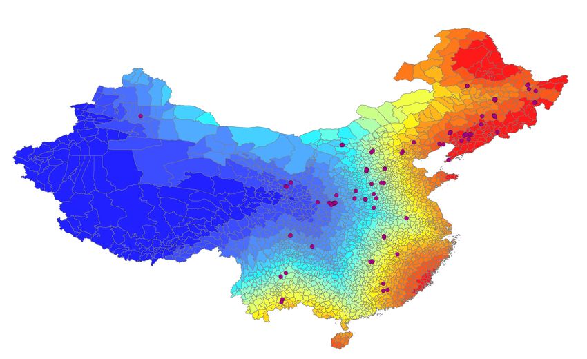

of Dutch disease (Corden and Neary, 1982), with an inefficient provision of factors
across production units and high production costs (Duranton, 2011).7 We find that:
labor costs are low but dispersed across production units; firms competing for the
same local resources as MRPs are not smaller or less numerous than similar industries
in control counties (in contrast with Falck et al., 2013); and the accumulation of
human capital is not negatively distorted (in contrast with Glaeser, 2005; Polèse,
2009; Franck and Galor, 2017). Third, the boom-and-bust is not driven by the
boom-and-bust of State-Owned-Enterprises (SOEs) over the period (Brandt et al.,
2016): if anything, SOEs in treated counties appear to be productive and innovative,
and our findings are mostly driven by private establishments. Fourth, the MRPs
may affect the local political environment. Corruption and political interventions
have been found to influence the competition for resources at the local level (Chen
et al., 2017; Wen, 2019) and MRPs may benefit for instance from favoritism and
preferential access to capital (Fang et al., 2018; Harrison et al., 2019). We find little
support for such interpretation: the other manufacturing establishments in treated
counties are capital-abundant, and the provision of subsidies does not appear to be
distorted towards public or linked establishments. Fifth, we control for the life-cycle
of establishments (Mueller, 1972) and for industry- and product-fixed-effects to clean
our findings from a rise and fall pattern due to the demographics of production units
or the boom and bust of certain production sectors.
    The research relates to the literature on agglomeration economies and urban
growth (see Duranton and Puga, 2014, for a review). Our contribution is close
to Greenstone et al. (2010), looking at the effect of Million-Dollar plants in the
United States, and to recent contributions analyzing the positive effects of early,
large industrialization (Mitrunen, 2019; Fan and Zou, 2019; Garin and Rothbaum,
2020; Méndez-Chacón and Van Patten, 2019). The distinct aspect of our study is to
document the negative impact of such investments in the longer run. In contrast to
most studies, we can also precisely characterize treatment spillovers by observing all
dimensions of treatment heterogeneity and micro-data at the establishment level.
    Our findings contribute to a recent body of research on place-based policies,
reviewed in Neumark and Simpson (2015), and including Busso et al. (2013), Kline
and Moretti (2014), von Ehrlich and Seidel (2018), Schweiger et al. (2018), Austin
et al. (2018), and Fajgelbaum and Gaubert (2020), by identifying the agglomeration
spillovers operating in the long run. Numerous contributions analyze the effect of
   7
      The analysis of the possible mechanisms through which MRPs may affect other establishments
relates to a large literature studying the credit market frictions (Hsieh and Klenow, 2009; Song
et al., 2011; Hsieh and Song, 2015; Brandt et al., 2016) and labor market frictions (Brandt et al.,
2013; Tombe and Zhu, 2019; Mayneris et al., 2018) in China.

                                                5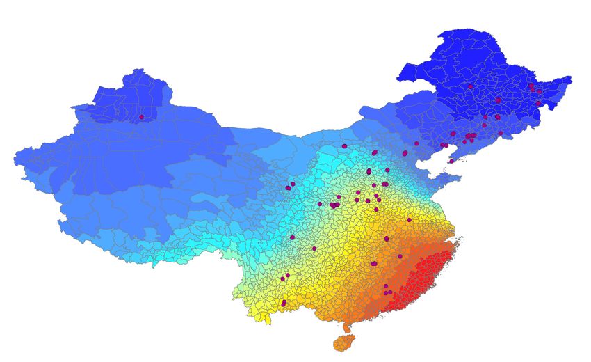

more recent spatial policies on the distribution of economic activity in China, for
instance, the Special Economic Zones and industrial parks (Wang, 2013; Crescenzi
et al., 2012; Alder et al., 2016; Zheng et al., 2017).
    Finally, identifying spillovers from local MRP(s) presents an econometric chal-
lenge. With treatment heterogeneity, i.e., with MRPs operating different technolo-
gies to produce different products and drawing on different factor markets, a simple
difference-in-differences procedure cannot be implemented: it would require us to
observe the sub-population of firms likely to be affected in control counties. We
specifically develop a two-step procedure to address this issue where (i) we stratify
counties by their propensity to receive a MRP, and (ii) we run Monte-Carlo sim-
ulations and draw—for each control county—one treated county (and its MRPs)
from the same stratum and hypothetically attribute the associated MRP(s) to the
control county. This empirical strategy could be useful to contributions analyzing
the spillovers of FDI on domestic firms (see, for instance, Head et al., 1995; Aitken
and Harrison, 1999; Konings, 2001; Smarzynska Javorcik, 2004; Haskel et al., 2007).
    The remainder of the paper is organized as follows. Section 1 describes the his-
torical context. Section 2 details the data and the empirical strategy. Section 3
presents empirical facts about the rise and fall of early-industrialized counties. Sec-
tion 4 provides evidence about the mechanisms behind the relative decline of treated
counties with more granular establishment-level data. Section 5 briefly concludes.

1     Historical background and the “156” program

The “156” program is a unique experiment to study agglomeration effects in the
long run. The program constitutes a massive push shock in an otherwise agrarian
economy (Lardy, 1987; Rawski, 1979); different types of factories were built thereby
allowing us to identify treatment heterogeneity. The geopolitical context introduces
unique exogenous variation in the decision to locate projects. The “156” program
was unanticipated before 1950, and strategic considerations behind the opening and
location of plants became irrelevant a few years later, after the Sino-Soviet Split.

1.1    The historical context

This section provides a brief account of the historical context; a comprehensive
description can be found in Appendix A.1.

Sino-Soviet cooperation (1950–1958) Although Sino-Soviet cooperation was
central in the first years of the People’s Republic, it was not based on strong pre-

                                          6

existing economic relations. In 1949, after decades of destruction through the Sino-
Japanese and Chinese civil wars, Chinese leaders studied the possibility of inter-
national economic cooperation to foster the development of heavy industry and
transform China’s agrarian economy. For geopolitical and ideological reasons,8 the
Chinese government engaged in economic cooperation with the Soviet Union to
give China its own independent industrial system (Dong, 1999; Lüthi, 2010). The
possibility of economic cooperation became credible after the Sino-Soviet Treaty of
Friendship and Alliance of 1950, which included a large loan. In August 1952, Chi-
nese Premier Zhou Enlai visited Moscow to formalize the involvement of the Soviet
Union in the long-delayed First Five-Year Plan (1953–1957). The U.S.S.R. agreed
to cooperate and assist China in the creation of state-of-the-art industrial sites, with
the purpose of extending its influence in the region.

Sino-Soviet Split (1958–1960) Rapid ideological and geopolitical divergence
precipitated a Sino-Soviet split that ended all cooperation between the two countries.
The split formally unfolded in 1960 with (i) an abrupt termination of industrial
collaboration and (ii) heightened military tensions. The termination of industrial
collaboration materialized in the sudden withdrawal of experts and engineers from
China, the repatriation of Chinese students from the U.S.S.R., and the cancellation
of ongoing industrial projects. The only remnants of the short-lived Sino-Soviet
alliance were 150 plants that had been already completed and were operational by
1960. The end of the military alliance also affected later industrial investment in
China. Before the Sino-Soviet Split, proximity to military U.S.S.R. air bases would
guarantee security against possible aerial attacks from the United States or from
the Republic of China relocated in Taiwan. After the Sino-Soviet Split, U.S.S.R. air
bases would be considered another threat, thereby explaining the peculiar features
of later strategic decisions (e.g., the Third Front Movement).

1.2    The “156” program

This section summarizes the key features of the “156” program; a comprehensive
description can be found in Appendix A.2. We also provide a more systematic
description of later place-based policies in Appendix A.3, and we derive descriptive
statistics about the MRPs in Appendix A.4.
   8
     The regime’s revolutionary agenda, American support for the Nationalist government in Tai-
wan in the aftermath of the civil war, the Western embargo (Zhang, 2001) and then the Korean
War, in which China directly participated by sending troops, reinforced links between China and
the Soviet Union. This policy was called “leaning to one side” (yi bian dao) by Chairman Mao in
a famous speech (“On the People’s Democratic Dictatorship”) delivered on June 30, 1949.

                                              7

An industrial collaboration As part of the First Five-Year Plan (1953–1957),
the U.S.S.R. committed to assisting China in the construction of 50 industrial sites.
In May 1953, 91 new projects were agreed on and an additional 15 in October
1954. Overall, about 150 state-of-the-art factories would be constructed between
1953 and 1958; the factories were huge investments and benefited from economic
and technological assistance from the Soviet Union.
    The U.S.S.R. actively participated in the design and construction of these fac-
tories. First, the economic aid from the U.S.S.R. extended beyond large loans; the
U.S.S.R. provided more than half of the required equipment.9 Second, the collabo-
ration involved the exchange of information, human capital, and technology (as in
the Marshall plans, see Giorcelli, 2019). During the peak of the cooperation, 20,000
scientific, industrial and technical experts from the Soviet Union lived and worked
in China to design the construction of factories and rationalize production (Zhang,
2001; Wang, 2003). In order to build capabilities, 80,000 Chinese students were
trained in Soviet universities and technological institutes. While some blueprints
were destroyed, the existing technology could be imitated and represented a large
shift in the technological frontier for an agrarian economy (Bo, 1991).10
    Chinese scholars credit the “156” program with having (i) invested in basic sec-
tors such as the energy and steel industries and laid the foundations for the develop-
ment of other industries, (ii) boosted production capacity and shifted the technolog-
ical frontier, and (iii) promoted a more even spatial development by industrializing
central and western provinces (Dong and Wu, 2004; Zhang, 2009; Shi, 2013; He and
Zhou, 2007). While these factories are known as the “156” in China, we rather
refer to them as the “Million-Rouble Plants” (MRPs). Indeed, at the time of the
Sino-Soviet Split, six factories were not yet viable and were forcefully closed; only
150 plants had been completed and were operational by 1960.

Location decisions The MRPs were regarded as iconic firms and planners put
much thought in siting decisions. First, planners selected locations using economic
criteria. These suitability criteria, detailed in Bo (1991), are: (i) connection to
the transportation network and access to markets, (ii) access to natural resources
through existing roads and rail, and (iii) belonging to an agrarian province, as the
investments were seen as an opportunity to smooth the spatial distribution of income.
   9
      As a payment, China was to give 140,000 tons of tungsten concentrate, 110,000 tons of tin,
35,000 tons of molybdenum concentrate, 30,000 tons of antimony, 90,000 tons of rubber and other
produce including wool, rice or tea. Some low-skilled workers were also sent to Siberia.
   10
      The last 15 projects agreed on in 1954 even benefited from state-of-the-art equipment that few
Soviet factories enjoyed (Goncharenko, 2002), allowing China to make the most of Gerschenkron’s
(1962) “advantage of backwardness” (Tang, 2009).

                                                 8

We will use these criteria to identify a relevant set of suitable counties.
    However, this period was an era of heightened geopolitical tensions that culmi-
nated in the Korean War—where U.S. soldiers and Chinese “volunteers” directly
confronted. Planners were concerned that the brand-new plants might become the
target of enemy attacks. The decision process involved senior military officials to de-
cide where factories should be built, accounting for the locations of enemy and allied
air bases. Major enemy air bases in Japan, South Korea and Taiwan were remnants
of the major U.S. air bases used during World War II, the Korean War, and bases
used by the United States Taiwan Defense Command. Most of the Chinese territory
was in the range of U.S. strategic bombers; the decision process thus heavily relied
on the locations of allied air bases, mostly in the Soviet Union and North Korea,
able to intercept them. As explained earlier, the Sino-Soviet split made this location
criterion redundant.

Million-Rouble Plants and economic growth For the first 30 years of their
existence, the MRPs developed in a planned economy. These factories and their
local economies were fueled by the provisions of the plan. Factor movement was not
free, and if more workers or capital could be productively employed, the plan would
reallocate resources. The command-economy era as a whole will be considered as the
treatment; treated counties enjoyed a head start at the onset of the reform period.
    Reforms to deregulate the economy were introduced in the 1980s. Private firms
could be set up and a dual price system allowed market transactions alongside the
old quota requirements. In the 1990s, restrictions on labor mobility were gradually
loosened, and migration began to rise as a major feature of Chinese economic growth.
The MRPs successfully adapted to the market economy and remained leaders in their
respective industries.11 These industrial clusters have diversified their activities,
their products ranging from computer screens to carrier-based aircraft.

2    Data and empirical strategy

This section describes data sources, the empirical strategy and provides some de-
scriptive statistics.
    11
     We provide evidence for the continued success of MRPs in Appendix A.4. Note, however, that
a small number of firms went bankrupt. Nine factories have been closed, all coal or non-ferrous
metal mines. Two other firms, a paper mill and a former military electronics plant, were partly
restructured and continue to operate. When construction plans were made in the 1950s, most
plants were built in the city center. As pollution issues and the need for expansion had not been
anticipated, nine plants were moved to the suburbs, within the same counties.

                                               9

2.1    Data

One requirement for estimating the long-term agglomeration effects of the opening of
large plants is to collect local data on economic production, ideally covering 60 years
from 1950 to 2015. In this paper, we mobilize the following main data sources: (a)
information on the Million-Rouble Plants and their evolution over time, (b) county-
level data on population and production (1953–2015), (c) establishment-level data
in recent years (1992–2008), linked with patent applications and other product-level
information (factor intensities and technological content), and (d) information on
entrepreneurship from population census data.

The Million-Rouble Plants In order to define the local treatment induced by
the presence of an industrial cluster, we collect information on the geo-coded loca-
tion of the factories that constitute the “156” program, information on the timing
of construction, the initial investment, the original industry, and the evolution of
production over time. These pieces of information are extracted primarily from Bo
(1991) and Dong and Wu (2004), and from historical archives, while the recent activ-
ity of these factories is retrieved using establishment-level data (see Appendix A.4).

County-level data We rely on Population Censuses in 1953, 1964, 1982, 1990,
2000, and 2010, nested at the county level.12 The 1953 data only provide popula-
tion and household counts, but subsequent censuses capture the agricultural status
of households. At the time of the command economy, the household registration
(hukou) type is a faithful reflection of both activity and the environment of residence.
This piece of information offers us the opportunity to start tracking the evolution
of urbanization and economic sectors from 1964 onward. Additional county-level
information is available in 1982, most notably a disaggregation of employment by
broad sectors and measures of output. In 1990, precise data are collected on the
sector and type of employment and occupation, as well as on housing and migration,
a phenomenon that mostly involved agricultural-hukou holders moving to cities in
search of better earning opportunities. The 2000 and 2010 Censuses further include
information on the place of residence five years earlier, timing of the last migration
spell, reason for migrating, and place and type of household registration.13
  12
       County gazetteers, which provide information on industrial and agricultural production, pop-
ulation, education, age, gender, and broad sector of activity, are currently being digitized and
harmonized as part of the China Gazetteer Project—see https://www.chinagazetteer.com/.
    13
       Data collected by statistical offices—gazetteers, censuses, surveys, and yearbooks—rely on
official administrative divisions at the time of data collection. County boundaries are subject to
frequent and sometimes substantial changes in China. To deal with this issue, we use the 2010
administrative map of China as our benchmark and re-weight the data collected in other years to

                                                10

Establishment-level data We rely on the National Bureau of Statistics (NBS)
“above-scale” firm data, which constitute a longitudinal census of all state-owned
manufacturing enterprises (SOEs) and of all non-SOEs manufacturing establish-
ments, as long as their annual sales exceed RMB 5 million, over the period 1992–
2008.14 We use the establishment data to: (i) infer linkages between establishments
and create measures of product concentration; (ii) estimate factor productivity; (iii)
observe technological innovations; and (iv) create measures of mark-ups to capture
product competition. We first rely on a text analysis based on the description of
products in order to associate a unique product code to each establishment and cre-
ate measures of product concentration (see Appendix B.1). We further complement
the establishment data with product-level information, in particular a benchmark
input-output matrix (United States, 2000), measures of technological closeness using
patenting in the United States (Bloom et al., 2013), and the revealed factor inten-
sity using the factor endowments of countries producing each good (Shirotori et al.,
2010). We use the production functions derived in Imbert et al. (2020) to measure
factor productivity (see Appendix B.2). We use the link provided by He et al. (2018)
to match establishments with patent applications across three categories of patents
(utility, invention, and design), and we rely on the procedure of De Loecker and
Warzynski (2012) to estimate mark-ups (see Appendix B.3).

2.2    Empirical strategy

This section describes the two steps of the baseline empirical strategy. We first
select counties based on their suitability for hosting a Million-Rouble Plant. We
then discuss how we construct a measure of vulnerability to enemy bombings and
use it to explain the choice of industry locations among suitable counties.

Propensity score and suitable locations We isolate a group of suitable coun-
ties by implementing a propensity-score matching based on the eligibility criteria
described in Bo (1991). The first criterion is market access and connectedness to
the transportation network. In the baseline matching procedure, we rely on an in-
match the 2010 borders. More precisely, we overlay the 2010 map with the map for every other
year y and create a new map with all the polygons defined by the 2010 and year-y divisions. We
then compute the area-weighted value of the variable of interest for each polygon and collapse the
values at the level of the 2010 counties.
   14
      These data cover and contain a wealth of accounting information at the level of “legal units.”
A legal unit can be a subsidiary of a firm, but has its own name and is financially independent
(Brandt et al., 2014). Nearly 97% of legal units in our data corresponded to single plants; we will
refer to these units as establishments. Unique establishment identifiers can be retrieved thanks
to the algorithm designed by Brandt et al. (2014) and extended in Imbert et al. (2020), thereby
allowing us to construct a panel of firms spanning the period 1992–2008.

                                                11

dicator variable that equals 1 if a county belongs to the provincial capital,15 county
population at baseline (measured by the 1953 Census) and county area to capture
the former. We construct a measure of proximity to a railroad hub, using the ex-
isting railroad network in 1948, to model connectedness. The second criterion is
access to resources which we proxy with measures of travel time to coal, ore and
coke deposits, through the transportation network in 1948 (see Appendix C.1). As
apparent in Appendix Figure C1, the historical development of the railway network
and the location of natural resources induces that a crescent of counties are prone
to receiving large industrial infrastructure. This crescent, located a few hundred
kilometers from the Eastern coasts and borders, may be interpreted as a Second
Front for industrialization; the later Third Front Movement will go deeper into the
hinterland—a decision that will be rationalized by our empirical strategy.16
    We regress the treatment, i.e., being in the close neighborhood of one of the
MRPs (within 20 kilometers), on the location determinants described above, Hc ,
to generate a propensity measure Pc = P (Hc ) for each county. We define the set
of suitable locations C = {c1 , . . . , cN } by matching treated counties with the five
nearest neighbors in terms of the propensity Pc . We restrict the matching proce-
dure to counties with a measure Pc in the support of the treated group. We impose
that matched control counties be selected outside the immediate vicinity of treated
counties, in order to avoid spillover effects into the control group. In the baseline,
we exclude counties whose centroids lie within a 4-degrees × 4-degrees rectangle—
roughly 2-3 times the size of the average prefecture—centered on a treated county.
We provide a more comprehensive description of the matching procedure in Ap-
pendix C.1 where we show the distribution of propensity scores and the balance of
matching variables within the selected sample of suitable counties.
    The geographic dispersion of the treated and control counties is shown in Fig-
ure 1: most treated and control counties are located along this “Second Front”
   15
      We consider a county as part of the provincial capital if it belongs to the prefecture in which
the provincial capital was located at the time of the First Five-Year Plan.
   16
      Although they do not feature among the list of explicit determinants, other geographical and
economic factors may have entered siting decisions, e.g., distance to major ports, and we condition
our analysis on factors susceptible to affect long-term economic growth in the baseline strategy
and in robustness checks. It is also worth noting that siting decisions were certainly informed
by little more, and perhaps much less, than our GIS measures. The lack of a well-functioning
statistical administration, which explains the delay in devising the First Five-Year Plan (1953–
1957), put severe constraints on policy making in the early years of the People’s Republic of China.
Finally, in the current strategy, few county characteristics are targeted thus leaving many variables
available for a balance test. By contrast, more variables could be used to refine the initial matching,
thereby leaving few characteristics to compare across treatment and control groups in an “over-
identification” check. We will show that our findings are not sensitive to small variations around
the baseline matching procedure.

                                                  12

crescent, treated counties are however less likely to be located in Central China.

Vulnerability To isolate exogenous variation in the decision to select counties, we
construct measures of vulnerability to airstrikes from U.S. and Taiwanese air bases,
accounting for the presence of allied bases acting as a shield.
    To this end, we geo-locate active U.S. Air Force bases and Taiwanese military
airfields (enemy air bases), as well as major U.S.S.R. and North Korean air bases
(allied air bases). To account for the presence of allied air bases, we penalize travel
time for enemy bombers in the vicinity of U.S.S.R. and North Korean bases. The
procedure, discussed in Appendix C.2, is disciplined by the technical characteristics
of jet fighters at that time, most notably their range, and produces a continuous
measure of the cost for enemy airplanes of traveling through any given point of the
Chinese territory. We compute the minimum travel cost from each active U.S.A.F.
or Taiwanese base to each county and define the measure of vulnerability Vc as the
minimum of penalized distances across all enemy bases.
    We illustrate the spatial variation in vulnerability to aerial attacks in Figure 2:
Panel (a) shows vulnerability in 1953, i.e., before the Sino-Soviet split, and Panel (b)
shows vulnerability after the split, in 1964. Military concerns should favor the
Northeast at the expense of Central China in 1953; the set of suitable and protected
locations however became much smaller after 1960, and investment during the Third
Front had to be targeted toward interior provinces. The paths of surveillance flights
between 1963 and 1965 (Panel d) provides a rationale for the decision to shield
the MRPs and the later Third Front factories: U.S. reconnaissance aircraft were
targeting some of these factories and the “Second Front” was not protected anymore
after the Sino-Soviet split. Our empirical strategy uses the pre-split measure as an
instrument for factory location decisions, conditioning for the post-split measure,
thereby leveraging the ephemeral alliance between China and the U.S.S.R. as the
main source of identification.

First stage Figure 3 provides a representation of the relationship between the
unconditional and the conditional proximity to U.S. and Taiwanese airbases and
factory location choices. Although we find both treated and control counties at most
levels of vulnerability, the distribution of travel cost across treated counties has a
much fatter right tail than that of the control group, which shows that factories were
preferably established at a (penalized) distance from enemy threats.
    The relationship between the treatment and vulnerability measure constitutes
the first stage of our empirical specification. Table 1 shows that vulnerability to

                                          13

enemy bombings is a crucial factor in the location choice. One additional stan-
dard deviation in penalized distance from enemy bases increases the propensity to
host a Million-Rouble plant by about 26 percentage points among suitable counties.
The average difference in vulnerability between treated and control counties is about
three quarters of a standard deviation; our instrument thus explains 0.75×26 ≈ 20%
of the allocation of MRPs among suitable counties. Table 1 displays three specifi-
cations, one without any controls (column 1), one with the propensity controls only
(column 2), and one with the full set of controls (baseline specification, column 3).
All specifications are restricted to the set of treated and control counties defined
by matching on access to natural resources and the additional economic and geo-
graphical determinants. The full set of controls is used to condition the analysis on
characteristics that may directly affect outcomes of interest in the second stage; it
is however reassuring that the first stage is not dependent on their inclusion.
    Importantly, while there is a strong relationship between our treatment (i.e., a
place-based policy between 1953–1958) and the vulnerability to aerial attacks in
1953, the treatment is not correlated with vulnerability measures as computed in
1964 and 1972. Furthermore, vulnerability to aerial attacks in 1953 does not strongly
correlate with later place-based policies. The geography of our place-based policy is
unrelated to the geography of later investments (see Appendix D.1).

Benchmark specification Let c denote a county and Tc the treatment variable
indicating whether a county hosts a factory. We estimate the following IV specifi-
cation on the sample of suitable counties:

                            Yc = β0 + β1 Tc + Xc βx + εc                          (1)

where Tc is instrumented by Vc , and Yc is a measure of economic activity at the
county level. The controls include the propensity controls, a set of propensity score
dummies (stratifying the sample along the propensity score), and the following ad-
ditional controls: travel cost to major ports, proximity to cities in 1900, proximity
to Ming-dynasty courier stations, distance to military airfields, and the post-split
vulnerability to air strikes. Standard errors are clustered at the level of 4-degree ×
4-degree cells.
    A key assumption underlying the empirical strategy is that the instrument has no
effect on outcomes of interest other than through the location of the Million-Rouble
plants. We now discuss possible concerns with this assumption. First, the respec-
tive locations of military bases could have influenced investment at later stages of
the Chinese structural transformation. Conditioning by the same vulnerability to

                                         14

enemy raids, but after the Sino-Soviet Split and the start of the Vietnam War re-
balanced the geographic distribution of military power in the region, should reduce
this concern. We also provide a sensitivity analysis by controlling for later spatial
policies and large shocks (e.g., Third Front Movement, Cultural Revolution, Special
Economic Zones, industrial parks etc.). Second, vulnerability may correlate with un-
observed county amenities, which would explain both the decision to locate factories
and be correlated with later patterns of economic growth. We control for elevation,
ruggedness, indicators of soil quality, and expected crop yield in robustness checks.
Third, vulnerability may correlate with the geography of the recent growth patterns
in China. For instance, China’s Southeast was considered vulnerable but widely
benefited from the opening of Chinese ports to trade in the reform era.17 Such a
violation of the exclusion restriction would induce a spurious negative correlation
between economic growth and the presence of “156”-program industries in the re-
form period. To deal with this concern, we will run a series of robustness checks,
most notably excluding a buffer around the Pearl river delta, excluding all Chinese
counties below a certain latitude, or controlling for distance to the coast. Fourth, we
can repeat our exercise by replacing actual factories with unfinished projects. While
the first stage still applies, the second stage shows no differences between placebo
locations and other suitable locations.

2.3    Descriptive statistics

The Million-Rouble Plants expanded and modernized the Chinese industry in a wide
range of sectors, but with a bias towards heavy, extractive, and energy industries
(e.g., coal mining or power plants, see Table 2).18 Construction started between 1953
and 1955, and was achieved at the latest in the first quarter of 1959. The last two
columns of Table 2 show planned and actual investment; the figures attest the scale
of the program for an agrarian economy like China in the 1950s. The average planned
investment by factory was about 100,000,000 yuan, which amounted to 15,000,000
Soviet roubles in 1957 ($120,000,000 in 2010 U.S. dollars); total investment was of
the order of a fourth of annual production in 1955.
    Table 3 provides key descriptive statistics for treated and control counties. About
5% of Chinese counties are defined as being treated, and we use 15% of Chinese
  17
      Note, however, that the vulnerability measure does not overlap with the coast-interior divide
that characterizes the spatial distribution of economic activity in China. Some factories were indeed
set up on the coast, first and foremost in Dalian, but not on the southern shore, too exposed to
American or Taiwanese strikes.
   18
      The “156” program follows the “Russian model” of industrialization (Rosenstein-Rodan,
1943), with coordinated and large investments across industries to modernize agrarian economies.
These upstream factories were expected to irrigate the economy downstream.

                                                 15

counties as suitable control counties in our baseline specification. As expected from
a context of heightened international tensions in Asia following the Korean War,
treated counties are located at a much greater distance from U.S.A.F. and Taiwanese
bases. The difference in mean penalized distance between treated places and the
average Chinese county is about 75% of a standard deviation. Note, however, that
control and treated counties do not differ markedly in their exposure to enemy raids
after the Sino-Soviet split.
    Differences in terms of population are small at baseline (1953), jump in 1964 and
stabilize somewhat afterwards. Descriptive statistics about urban registration show
a similar gradient between treated and control locations, albeit more persistent.
Households in treated counties are more likely to hold an urban registration even
after the reform. These differences are, however, not indicative of economic activity
from 1990 onward, given the large number of rural migrants working in cities.
    The bottom panels of Table 3 describes possible differences in matching variables
and additional controls used in the baseline. Consistent with the propensity match-
ing procedure, differences in topography and connectedness are less pronounced
among suitable locations. Treated counties exhibit slightly lower travel costs to
coal, coke and ore deposits. These differences are nonetheless accounted for by
propensity-bin dummies and matching weights in Specification (1). Two historical
control variables appear as being important in explaining the allocation of treat-
ment, even though they do not explicitly feature among location criteria: proximity
to cities in 1900 and proximity to Ming stations. We thus include these variables as
controls in the baseline specification.

3     The rise-and-fall pattern

This section presents the implications of early industrialization in 1982 and in 2010.

3.1      Baseline results

The influence of the Million-Rouble plants on local trajectories spans two different
periods: the rise in the command-economy and the fall during the reform period.19

The rise We first describe empirical facts about the local treatment effect of in-
dustrial clusters in 1982; the analysis and the choice of outcomes are unfortunately
    19
     Note that reforms in the non-agricultural sector were introduced gradually. Private firms were
allowed to develop and compete with state-owned enterprises (SOEs) from the mid-1980s onward,
which was instrumental in introducing market discipline in state-owned enterprises. Nonetheless,
the large privatization wave did not start until the 1990s.

                                                16

limited by the availability of information at the county level. Table 4 shows OLS
(Panel A) and IV estimates (Panel B) of the relationship between the presence of a
MRP and population, share of urban residents, output per capita, and the employ-
ment share in industry (in 1982 and in 2010).
    We find that industrial investment under the “156” program has a positive and
significant impact, albeit small, on population in the earlier period. Treated counties
are 22% more populated than control counties (column 1, Panel B). The treatment
effect on urbanization is much larger; the share of the population that has non-
agricultural household registration is about 35 percentage points higher (column 2,
Panel B). The impact of the MRPs shows a large reallocation of labor, which could
be interpreted as evidence of structural transformation and urbanization. The higher
share of urban residents is associated with a much higher output per capita, and
a higher industry share in the local economy (columns 3 and 4, Panel B). GDP
per capita is more than twice larger in treated counties; the employment share in
industry is 24 percentage points higher. The magnitude of these differences is far
beyond the mere output of the average MRP, indicating that counties are richer and
more developed—the effect is equivalent to the difference between the median and
the top 10% of the control-group distribution.
    A few remarks are in order. First, the IV estimates are larger than the OLS esti-
mates, possibly reflecting that places selected to host a MRP were less likely to host
major industrial developments prior to the First Five-Year Plan (Bo, 1991). Second,
the extent of the short-run impact of industrial clusters may have limited external
validity. Before the advent of the reforms, the government would instruct workers
where to live and where to work to accommodate rising demand for labor and ensure
the growth of the plants and local economy.20 Changes in labor allocation mostly
reflect government intervention, which is likely to temper agglomeration effects. The
population increase, while larger than the expected labor force of the MRP itself,
remains limited and probably lags behind labor demand in treated counties.
    To summarize the impact of the “156” program between 1953 and 1982, we find a
moderate effect on urban population, but a very large effect on the local structure of
production. The substantial productivity gap between treated and control counties
indicates that treated areas enter the subsequent period with a substantial head
start. Lower mobility costs and the liberalization of the economy should allow
agglomeration economies to operate, and one could expect treated counties to grow
  20
      While some free movement of labor still occurred after the advent of “New China” in 1949,
mobility was subject to authorization from the late 1950s onward. The government had tightened
its grip on labor movement in the wake of the Great Leap Forward, when famines threatened the
sustainability of urban food provision systems.

                                              17

even further apart from the rest of the economy. As we see next, we find the opposite.

The fall There is a full catch-up between 1982 and 2010 (see Table 4). We find that
population is still higher in treated counties (column 1, Panel B); treated locations
also continue to have a significantly higher share of urban population (column 2,
Panel B). In stark contrast with the treatment effect in 1982, however, output per
capita and the industry share are now similar or even lower in treated counties
(columns 3 and 4, Panel B). The significant gap in industrialization before the
transition has thus fully eroded: treated counties are equally productive as control
counties and the employment share in industry is 13 percentage points lower.
    This fast reversion to the mean is puzzling for two reasons. First, it does not
result from a swift decline in employment in the Million-Rouble plants themselves;
the MRPs remain very large and extremely productive.21 Second, their influence
on aggregate productivity is non-negligible: the previous results indicate that other
production units must be quite unproductive.22 Before turning to the mechanisms
underlying this stylized fact, we provide a series of robustness checks.

3.2    Robustness checks and sensitivity analysis

The empirical strategy exploits temporary, exogenous variation in the probability
to host a MRP among suitable counties. The geographical variation induced by the
vulnerability to bombing between 1950–1960 may however coincidentally correlate
with other geographic determinants of later economic growth. This section provides
a comprehensive sensitivity analysis to reduce concerns that the rise and the fall
are related to other factors than the allocation of MRPs itself. We summarize these
robustness checks below and leave a detailed discussion of the results along with
additional Figures and Tables to Appendix D.1.
    We interpret the previous estimates as the effect of MRPs on the local economy.
One concern is that the instrument, which relies on the distribution of air bases
across space, may correlate with other geographic factors that have independent
effects on the distribution of economic activity across China and over time: (i) the
spatial distribution of market access (including exports), access to resources, land
supply; and (ii) later spatial policies (e.g., Special Economic Zones, industrial parks).
  21
      In Appendix D.1, we exclude the few counties hosting closed and displaced factories to show
that the fall is not related to the fall of MRPs themselves—we also better account for MRP type
(e.g., extracting industries).
   22
      Appendix A.4 provides a comparison between the MRPs and similar “above-scale” manu-
facturing establishments, shows the dynamics of employment and patenting in these MRPs, and
derives estimates of their employment shares in their local economies.

                                               18

In Appendix D.1, we first condition the baseline specification on measures capturing
an environment that is (un)favorable to economic take-off (e.g., connectedness in
2010, trade routes, natural amenities, elevation, access to ports, distance to the
coast, soil characteristics, and crop yield) to reduce concerns about biasing effects
from unobserved county characteristics. Second, we exclude the Pearl river delta and
the South of China to show that our results are not driven by the overall geography
of the economic take-off in China. Third, we control for later place-based policies
which could reduce the gap between treated and control counties (e.g., Third Front
Movement, Special Economic Zones, or industrial parks), for factors underlying these
later decisions (e.g., vulnerability to U.S.S.R. strikes), and for other large policy
shocks driving the economic evolution of China (e.g., the Cultural Revolution).
    We also consider variations in our matching procedure and the use of matching
weights. We extend the set of variables used for matching by adding proximity to
Ming stations, distance to military airfields and access to the main trading ports;
we then restrict the set to a minimum set of variables: travel cost to coal mines,
proximity to a rail hub, whether the county is a provincial capital, population in 1953
(log), and county area (log). We further restrict the choice of control counties by
considering a one-to-one matching procedure without replacement, and by enlarging
the exclusion zone around treated counties. We also provide a sensitivity analysis
around the construction of the vulnerability instrument and around the treatment
of spatial auto-correlation.
    Finally, we consider alternative measures of economic activity, including a more
precise sectoral analysis and the use of nighttime luminosity in 1993 and in 2013.
We also provide some insight on the dynamics from 1990 onward showing that there
is a gradual decrease in economic activity in treated counties.

3.3   The (dramatic) fall of other establishments

Treated counties experience a swift reversion to the mean in aggregate output. The
dynamics of the local economy is however strongly driven by the dynamics of MRPs
themselves, and these MRPs experience, for instance, an increase in patenting ac-
tivity in the recent period. We now rely on micro-data to better characterize the
structure of production in the average other establishment. The analysis relies on:
measures of factor productivity at the establishment level, identified using an exoge-
nous labor supply shifter (see Imbert et al., 2020, and Appendix B.2); patents linked
to establishments (He et al., 2018); and markups computed following De Loecker

                                          19

and Warzynski (2012) (see Appendix B.3).23
    In Table 5, we extend Specification (1) at the establishment-level, consider all
establishment × year observations between 1992 and 2008, and regress a measure of
production on the treatment Tc , instrumented by Vc . We clean for year interacted
with 4-digit industry fixed effects and for year interacted with firm type: our results
are orthogonal to aggregate industrial trends and to the demise of public establish-
ments. We also exclude the MRPs from the sample and we cluster standard errors
at the level of 4-degree × 4-degree cells.
    Factor use is different in treated and in control counties (columns 1 and 2): es-
tablishments in treated counties are more capital-abundant than in control counties;
real capital is 40% higher, while employment is 30% higher. Labor cost sharply dif-
fers in treated counties. We find that the average compensation per employee is
about 32% lower in treated counties (Table 5, column 3). These findings point to a
downward shift in labor supply in treated counties compared to control counties.
    Total factor productivity is 30% lower in treated counties than in control counties
(Table 5, column 4).24 This finding could either indicate that the treatment generates
differences in technology adoption or differences in price setting between control
and treated counties. We investigate these two aspects next. While we distinguish
three patent categories in Appendix D.3 (design, innovation, and utility—the latter
categories being the most relevant to capture technological progress), we only report
the treatment effect on the total number of registered utility patent applications in
column 5 of Table 5. We find that establishments in treated counties produce fewer
patents. The treatment effect is of the order of magnitude of the yearly number
of patents produced in the average establishment: very few patents are registered
in treated counties.25 Finally, as shown in column 6 of Table 5, the TFP effect
cannot be explained by markups; they are on average higher in treated counties:
the probability for a firm to charge a markup above median in a given year and
4-digit industry is 13 percentage points higher in treated counties.
    The previous results cannot be attributed to compositional differences induced
by the presence of public enterprises, subsidized establishments (Harrison et al.,
2019), or young firms. Indeed, (i) controlling for the exact type of an establishment
   23
      In this section, we describe the treatment effect on the structure of production using a se-
lection of outcomes, and we leave the detailed analysis of factor use, factor productivity, firm
characteristics, investment and subsidies, patenting behavior, and price setting in Appendix D.3.
   24
      Labor cost and factor productivity appear to be low in treated counties, but dispersed (see
Appendix D.3).
   25
      Controlling for the local industry structure is innocuous for factor productivity and factor use
but quite important for patenting behavior. Indeed, the presence of the MRP(s) tilts the local
industrial fabric toward innovative sectors; these innovative sectors are however far less innovative
in treated counties.

                                                 20