Beyond Bags of Features: Spatial Pyramid Matching for Recognizing Natural Scene Categories
←
→
Page content transcription
If your browser does not render page correctly, please read the page content below

Beyond Bags of Features: Spatial Pyramid Matching
                          for Recognizing Natural Scene Categories

             Svetlana Lazebnik1                     Cordelia Schmid2                         Jean Ponce1,3
                slazebni@uiuc.edu              Cordelia.Schmid@inrialpes.fr                ponce@cs.uiuc.edu
                1                                   2                                3
                Beckman Institute                   INRIA Rhône-Alpes                   Ecole Normale Supérieure
               University of Illinois               Montbonnot, France                        Paris, France

                         Abstract                                 search [1, 11] achieve robustness at significant computa-
                                                                  tional expense. A more efficient approach is to augment a
    This paper presents a method for recognizing scene cat-       basic bag-of-features representation with pairwise relations
egories based on approximate global geometric correspon-          between neighboring local features, but existing implemen-
dence. This technique works by partitioning the image into        tations of this idea [11, 17] have yielded inconclusive re-
increasingly fine sub-regions and computing histograms of         sults. One other strategy for increasing robustness to geo-
local features found inside each sub-region. The result-          metric deformations is to increase the level of invariance of
ing “spatial pyramid” is a simple and computationally effi-       local features (e.g., by using affine-invariant detectors), but
cient extension of an orderless bag-of-features image rep-        a recent large-scale evaluation [25] suggests that this strat-
resentation, and it shows significantly improved perfor-          egy usually does not pay off.
mance on challenging scene categorization tasks. Specifi-             Though we remain sympathetic to the goal of develop-
cally, our proposed method exceeds the state of the art on        ing robust and geometrically invariant structural object rep-
the Caltech-101 database and achieves high accuracy on a          resentations, we propose in this paper to revisit “global”
large database of fifteen natural scene categories. The spa-      non-invariant representations based on aggregating statis-
tial pyramid framework also offers insights into the success      tics of local features over fixed subregions. We introduce a
of several recently proposed image descriptions, including        kernel-based recognition method that works by computing
Torralba’s “gist” and Lowe’s SIFT descriptors.                    rough geometric correspondence on a global scale using an
                                                                  efficient approximation technique adapted from the pyramid
                                                                  matching scheme of Grauman and Darrell [7]. Our method
1. Introduction                                                   involves repeatedly subdividing the image and computing
                                                                  histograms of local features at increasingly fine resolutions.
   In this paper, we consider the problem of recognizing
                                                                  As shown by experiments in Section 5, this simple oper-
the semantic category of an image. For example, we may
                                                                  ation suffices to significantly improve performance over a
want to classify a photograph as depicting a scene (forest,
                                                                  basic bag-of-features representation, and even over meth-
street, office, etc.) or as containing a certain object of in-
                                                                  ods based on detailed geometric correspondence.
terest. For such whole-image categorization tasks, bag-of-
features methods, which represent an image as an orderless           Previous research has shown that statistical properties of
collection of local features, have recently demonstrated im-      the scene considered in a holistic fashion, without any anal-
pressive levels of performance [7, 22, 23, 25]. However,          ysis of its constituent objects, yield a rich set of cues to its
because these methods disregard all information about the         semantic category [13]. Our own experiments confirm that
spatial layout of the features, they have severely limited de-    global representations can be surprisingly effective not only
scriptive ability. In particular, they are incapable of captur-   for identifying the overall scene, but also for categorizing
ing shape or of segmenting an object from its background.         images as containing specific objects, even when these ob-
Unfortunately, overcoming these limitations to build effec-       jects are embedded in heavy clutter and vary significantly
tive structural object descriptions has proven to be quite        in pose and appearance. This said, we do not advocate the
challenging, especially when the recognition system must          direct use of a global method for object recognition (except
be made to work in the presence of heavy clutter, occlu-          for very restricted sorts of imagery). Instead, we envision a
sion, or large viewpoint changes. Approaches based on             subordinate role for this method. It may be used to capture
generative part models [3, 5] and geometric correspondence        the “gist” of an image [21] and to inform the subsequent
search for specific objects (e.g., if the image, based on its    subdivision scheme (although a regular 4 × 4 grid seems
global description, is likely to be a highway, we have a high    to be the most popular implementation choice), and what is
probability of finding a car, but not a toaster). In addition,   the right balance between “subdividing” and “disordering.”
the simplicity and efficiency of our method, in combina-         The spatial pyramid framework suggests a possible way to
tion with its tendency to yield unexpectedly high recogni-       address this issue: namely, the best results may be achieved
tion rates on challenging data, could make it a good base-       when multiple resolutions are combined in a principled way.
line for “calibrating” new datasets and for evaluating more      It also suggests that the reason for the empirical success of
sophisticated recognition approaches.                            “subdivide and disorder” techniques is the fact that they ac-
                                                                 tually perform approximate geometric matching.
2. Previous Work
    In computer vision, histograms have a long history as a
method for image description (see, e.g., [16, 19]). Koen-        3. Spatial Pyramid Matching
derink and Van Doorn [10] have generalized histograms to
locally orderless images, or histogram-valued scale spaces          We first describe the original formulation of pyramid
(i.e., for each Gaussian aperture at a given location and        matching [7], and then introduce our application of this
scale, the locally orderless image returns the histogram of      framework to create a spatial pyramid image representation.
image features aggregated over that aperture). Our spatial
pyramid approach can be thought of as an alternative for-
mulation of a locally orderless image, where instead of a        3.1. Pyramid Match Kernels
Gaussian scale space of apertures, we define a fixed hier-
archy of rectangular windows. Koenderink and Van Doorn               Let X and Y be two sets of vectors in a d-dimensional
have argued persuasively that locally orderless images play      feature space. Grauman and Darrell [7] propose pyramid
an important role in visual perception. Our retrieval exper-     matching to find an approximate correspondence between
iments (Fig. 4) confirm that spatial pyramids can capture        these two sets. Informally, pyramid matching works by
perceptually salient features and suggest that “locally or-      placing a sequence of increasingly coarser grids over the
derless matching” may be a powerful mechanism for esti-          feature space and taking a weighted sum of the number of
mating overall perceptual similarity between images.             matches that occur at each level of resolution. At any fixed
    It is important to contrast our proposed approach with       resolution, two points are said to match if they fall into the
multiresolution histograms [8], which involve repeatedly         same cell of the grid; matches found at finer resolutions are
subsampling an image and computing a global histogram            weighted more highly than matches found at coarser resolu-
of pixel values at each new level. In other words, a mul-        tions. More specifically, let us construct a sequence of grids
tiresolution histogram varies the resolution at which the fea-   at resolutions 0, . . . , L, such that the grid at level  has 2
tures (intensity values) are computed, but the histogram res-    cells along each dimension, for a total of D = 2d cells. Let

olution (intensity scale) stays fixed. We take the opposite      HX   and HY denote the histograms of X and Y at this res-
approach of fixing the resolution at which the features are      olution, so that HX
                                                                                        (i) and HY (i) are the numbers of points
computed, but varying the spatial resolution at which they       from X and Y that fall into the ith cell of the grid. Then
are aggregated. This results in a higher-dimensional rep-        the number of matches at level  is given by the histogram
resentation that preserves more information (e.g., an image      intersection function [19]:
consisting of thin black and white stripes would retain two
modes at every level of a spatial pyramid, whereas it would
                                                                                           D

become indistinguishable from a uniformly gray image at                   I(HX

                                                                               , HY ) =         min HX (i), HY (i) .        (1)
all but the finest levels of a multiresolution histogram). Fi-                             i=1
nally, unlike a multiresolution histogram, a spatial pyramid,
when equipped with an appropriate kernel, can be used for
approximate geometric matching.                                  In the following, we will abbreviate I(HX

                                                                                                           , HY ) to I  .
    The operation of “subdivide and disorder” — i.e., par-          Note that the number of matches found at level  also in-
tition the image into subblocks and compute histograms           cludes all the matches found at the finer level  + 1. There-
(or histogram statistics, such as means) of local features in    fore, the number of new matches found at level  is given
these subblocks — has been practiced numerous times in           by I  − I +1 for  = 0, . . . , L − 1 . The weight associated
                                                                                          1
computer vision, both for global image description [6, 18,       with level  is set to 2L−  , which is inversely proportional
20, 21] and for local description of interest regions [12].      to cell width at that level. Intuitively, we want to penalize
Thus, though the operation itself seems fundamental, pre-        matches found in larger cells because they involve increas-
vious methods leave open the question of what is the right       ingly dissimilar features. Putting all the pieces together, we
level 0                        level 1                         level 2
get the following definition of a pyramid match kernel:                                    + +                               + +                             + +
                                                                                                           +                                 +                               +
                                                                                                       +                                 +                               +

                                       L−1
                                               1                                    +           +                     +          +                    +           +
        κL (X, Y )       = IL +                   I − I +1               (2)              +           +                     +           +                   +           +
                                             2L−
                                       =0                                         +                                 +                               +

                                1 0
                                           L
                                                   1
                         =        I +                   I .              (3)                          + +       +                       + +     +                       + +     +
                               2L                2L−+1
                                           =1                                                               +                               +                               +

Both the histogram intersection and the pyramid match ker-
nel are Mercer kernels [7].
                                                                                               ´ 1/4                             ´ 1/4                           ´ 1/2
3.2. Spatial Matching Scheme                                                     Figure 1. Toy example of constructing a three-level pyramid. The
                                                                                 image has three feature types, indicated by circles, diamonds, and
   As introduced in [7], a pyramid match kernel works                            crosses. At the top, we subdivide the image at three different lev-
with an orderless image representation. It allows for pre-                       els of resolution. Next, for each level of resolution and each chan-
cise matching of two collections of features in a high-                          nel, we count the features that fall in each spatial bin. Finally, we
dimensional appearance space, but discards all spatial in-                       weight each spatial histogram according to eq. (3).
formation. This paper advocates an “orthogonal” approach:
perform pyramid matching in the two-dimensional image                               The final implementation issue is that of normalization.
space, and use traditional clustering techniques in feature                      For maximum computational efficiency, we normalize all
space.1 Specifically, we quantize all feature vectors into M                     histograms by the total weight of all features in the image,
discrete types, and make the simplifying assumption that                         in effect forcing the total number of features in all images to
only features of the same type can be matched to one an-                         be the same. Because we use a dense feature representation
other. Each channel m gives us two sets of two-dimensional                       (see Section 4), and thus do not need to worry about spuri-
vectors, Xm and Ym , representing the coordinates of fea-                        ous feature detections resulting from clutter, this practice is
tures of type m found in the respective images. The final                        sufficient to deal with the effects of variable image size.
kernel is then the sum of the separate channel kernels:


                                    M
                K L (X, Y ) =             κL (Xm , Ym ) .                 (4)    4. Feature Extraction
                                   m=1
                                                                                    This section briefly describes the two kinds of features
This approach has the advantage of maintaining continuity                        used in the experiments of Section 5. First, we have so-
with the popular “visual vocabulary” paradigm — in fact, it                      called “weak features,” which are oriented edge points, i.e.,
reduces to a standard bag of features when L = 0.                                points whose gradient magnitude in a given direction ex-
    Because the pyramid match kernel (3) is simply a                             ceeds a minimum threshold. We extract edge points at two
weighted sum of histogram intersections, and because                             scales and eight orientations, for a total of M = 16 chan-
c min(a, b) = min(ca, cb) for positive numbers, we can                           nels. We designed these features to obtain a representation
implement K L as a single histogram intersection of “long”                       similar to the “gist” [21] or to a global SIFT descriptor [12]
vectors formed by concatenating the appropriately weighted                       of the image.
histograms of all channels at all resolutions (Fig. 1). For
                                                                                     For better discriminative power, we also utilize higher-
L levels and M channels, the resulting vector has dimen-
                                                                                 dimensional “strong features,” which are SIFT descriptors
sionality M =0 4 = M 13 (4L+1 − 1). Several experi-
                L
                                                                                 of 16 × 16 pixel patches computed over a grid with spacing
ments reported in Section 5 use the settings of M = 400
                                                                                 of 8 pixels. Our decision to use a dense regular grid in-
and L = 3, resulting in 34000-dimensional histogram in-
                                                                                 stead of interest points was based on the comparative evalu-
tersections. However, these operations are efficient because
                                                                                 ation of Fei-Fei and Perona [4], who have shown that dense
the histogram vectors are extremely sparse (in fact, just as
                                                                                 features work better for scene classification. Intuitively, a
in [7], the computational complexity of the kernel is linear
                                                                                 dense image description is necessary to capture uniform re-
in the number of features). It must also be noted that we did
                                                                                 gions such as sky, calm water, or road surface (to deal with
not observe any significant increase in performance beyond
                                                                                 low-contrast regions, we skip the usual SIFT normalization
M = 200 and L = 2, where the concatenated histograms
                                                                                 procedure when the overall gradient magnitude of the patch
are only 4200-dimensional.
                                                                                 is too weak). We perform k-means clustering of a random
    1 In principle, it is possible to integrate geometric information directly   subset of patches from the training set to form a visual vo-
into the original pyramid matching framework by treating image coordi-           cabulary. Typical vocabulary sizes for our experiments are
nates as two extra dimensions in the feature space.
                                                                                 M = 200 and M = 400.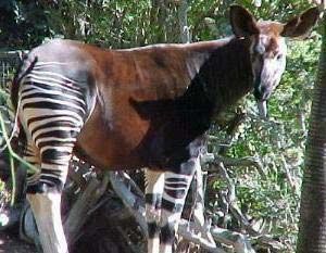
office                                              kitchen                                       living room

                        bedroom                                                    store                                     industrial

                     tall building∗                                        inside city∗                                        street∗

                       highway∗                                                coast∗                                     open country∗

                      mountain∗                                               forest∗                                         suburb
         Figure 2. Example images from the scene category database. The starred categories originate from Oliva and Torralba [13].

                                       Weak features (M = 16)             Strong features (M = 200)           Strong features (M = 400)
                       L         Single-level      Pyramid      Single-level      Pyramid        Single-level     Pyramid
                   0 (1 × 1)      45.3 ±0.5                      72.2 ±0.6                        74.8 ±0.3
                   1 (2 × 2)      53.6 ±0.3       56.2 ±0.6      77.9 ±0.6       79.0 ±0.5        78.8 ±0.4      80.1 ±0.5
                   2 (4 × 4)      61.7 ±0.6       64.7 ±0.7      79.4 ±0.3       81.1 ±0.3        79.7 ±0.5      81.4 ±0.5
                   3 (8 × 8)      63.3 ±0.8       66.8 ±0.6      77.2 ±0.4       80.7 ±0.3        77.2 ±0.5      81.1 ±0.6
Table 1. Classification results for the scene category database (see text). The highest results for each kind of feature are shown in bold.

5. Experiments                                                                             5.1. Scene Category Recognition

                                                                                               Our first dataset (Fig. 2) is composed of fifteen scene cat-
   In this section, we report results on three diverse
                                                                                           egories: thirteen were provided by Fei-Fei and Perona [4]
datasets: fifteen scene categories [4], Caltech-101 [3], and
                                                                                           (eight of these were originally collected by Oliva and Tor-
Graz [14]. We perform all processing in grayscale, even
                                                                                           ralba [13]), and two (industrial and store) were collected by
when color images are available. All experiments are re-
                                                                                           ourselves. Each category has 200 to 400 images, and av-
peated ten times with different randomly selected training
                                                                                           erage image size is 300 × 250 pixels. The major sources
and test images, and the average of per-class recognition
                                                                                           of the pictures in the dataset include the COREL collection,
rates2 is recorded for each run. The final result is reported as
                                                                                           personal photographs, and Google image search. This is
the mean and standard deviation of the results from the in-
                                                                                           one of the most complete scene category dataset used in the
dividual runs. Multi-class classification is done with a sup-
                                                                                           literature thus far.
port vector machine (SVM) trained using the one-versus-all
rule: a classifier is learned to separate each class from the                                 Table 1 shows detailed results of classification experi-
rest, and a test image is assigned the label of the classifier                             ments using 100 images per class for training and the rest
with the highest response.                                                                 for testing (the same setup as [4]). First, let us examine the
                                                                                           performance of strong features for L = 0 and M = 200,
                                                                                           corresponding to a standard bag of features. Our classi-
                                                                                           fication rate is 72.2% (74.7% for the 13 classes inherited
   2 The
                                                                                           from Fei-Fei and Perona), which is much higher than their
         alternative performance measure, the percentage of all test im-
                                                                                           best results of 65.2%, achieved with an orderless method
ages classified correctly, can be biased if test set sizes for different classes
vary significantly. This is especially true of the Caltech-101 dataset, where              and a feature set comparable to ours. We conjecture that
some of the “easiest” classes are disproportionately large.                                Fei-Fei and Perona’s approach is disadvantaged by its re-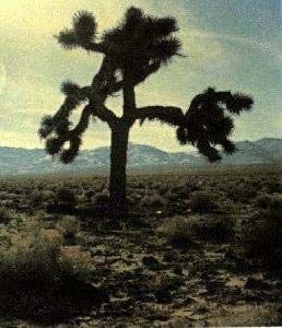
open country
together confers a statistically significant benefit. For strong
tall building
living room
inside city
mountain
industrial
bedroom
features, single-level performance actually drops as we go
highway
kitchen
suburb
street
forest
office
coast
from L = 2 to L = 3. This means that the highest level of
store
office 92.7
the L = 3 pyramid is too finely subdivided, with individ-
kitchen 68.5
ual bins yielding too few matches. Despite the diminished
living room 60.4
discriminative power of the highest level, the performance
bedroom 68.3 of the entire L = 3 pyramid remains essentially identical to
store 76.2 that of the L = 2 pyramid. This, then, is the main advantage
industrial 65.4 of the spatial pyramid representation: because it combines
tall building 91.1 multiple resolutions in a principled fashion, it is robust to
inside city 80.5 failures at individual levels.
street 90.2
It is also interesting to compare performance of differ-
highway 86.6
ent feature sets. As expected, weak features do not per-
coast 82.4
form as well as strong features, though in combination with
open country 70.5
the spatial pyramid, they can also achieve acceptable levels
mountain 88.8
of accuracy (note that because weak features have a much
forest 94.7
higher density and much smaller spatial extent than strong
suburb 99.4
features, their performance continues to improve as we go
Figure 3. Confusion table for the scene category dataset. Average from L = 2 to L = 3). Increasing the visual vocabulary
classification rates for individual classes are listed along the diag- size from M = 200 to M = 400 results in a small perfor-
onal. The entry in the ith row and jth column is the percentage of mance increase at L = 0, but this difference is all but elim-
images from class i that were misidentified as class j. inated at higher pyramid levels. Thus, we can conclude that
liance on latent Dirichlet allocation (LDA) [2], which is the coarse-grained geometric cues provided by the pyramid
essentially an unsupervised dimensionality reduction tech- have more discriminative power than an enlarged visual vo-
nique and as such, is not necessarily conducive to achiev- cabulary. Of course, the optimal way to exploit structure
ing the highest classification accuracy. To verify this, we both in the image and in the feature space may be to com-
have experimented with probabilistic latent semantic analy- bine them in a unified multiresolution framework; this is
sis (pLSA) [9], which attempts to explain the distribution of subject for future research.
features in the image as a mixture of a few “scene topics” Fig. 3 shows a confusion table between the fifteen scene
or “aspects” and performs very similarly to LDA in prac- categories. Not surprisingly, confusion occurs between the
tice [17]. Following the scheme of Quelhas et al. [15], we indoor classes (kitchen, bedroom, living room), and also be-
run pLSA in an unsupervised setting to learn a 60-aspect tween some natural classes, such as coast and open country.
model of half the training images. Next, we apply this Fig. 4 shows examples of image retrieval using the spatial
model to the other half to obtain probabilities of topics given pyramid kernel and strong features with M = 200. These
each image (thus reducing the dimensionality of the feature examples give a sense of the kind of visual information cap-
space from 200 to 60). Finally, we train the SVM on these tured by our approach. In particular, spatial pyramids seem
reduced features and use them to classify the test set. In this successful at capturing the organization of major pictorial
setup, our average classification rate drops to 63.3% from elements or “blobs,” and the directionality of dominant lines
the original 72.2%. For the 13 classes inherited from Fei- and edges. Because the pyramid is based on features com-
Fei and Perona, it drops to 65.9% from 74.7%, which is puted at the original image resolution, even high-frequency
now very similar to their results. Thus, we can see that la- details can be preserved. For example, query image (b)
tent factor analysis techniques can adversely affect classifi- shows white kitchen cabinet doors with dark borders. Three
cation performance, which is also consistent with the results of the retrieved “kitchen” images contain similar cabinets,
of Quelhas et al. [15]. the “office” image shows a wall plastered with white docu-
ments in dark frames, and the “inside city” image shows a
Next, let us examine the behavior of spatial pyramid
white building with darker window frames.
matching. For completeness, Table 1 lists the performance
achieved using just the highest level of the pyramid (the
5.2. Caltech-101
“single-level” columns), as well as the performance of the
complete matching scheme using multiple levels (the “pyra- Our second set of experiments is on the Caltech-101
mid” columns). For all three kinds of features, results im- database [3] (Fig. 5). This database contains from 31 to
prove dramatically as we go from L = 0 to a multi-level 800 images per category. Most images are medium resolu-
setup. Though matching at the highest pyramid level seems tion, i.e., about 300 × 300 pixels. Caltech-101 is probably
to account for most of the improvement, using all the levels the most diverse object database available today, though it
(a) kitchen      living room   living room   living room    office      living room    living room    living room    living room

        (b) kitchen                                                 office                                                    inside city

         (c) store                                                 mountain                       forest

        (d) tall bldg                                inside city                                               inside city

        (e) tall bldg    inside city                  mountain                                                 mountain       mountain

       (f) inside city                                tall bldg

         (g) street

Figure 4. Retrieval from the scene category database. The query images are on the left, and the eight images giving the highest values of
the spatial pyramid kernel (for L = 2, M = 200) are on the right. The actual class of incorrectly retrieved images is listed below them.

is not without shortcomings. Namely, most images feature                tures at L = 2. This exceeds the highest classification rate
relatively little clutter, and the objects are centered and oc-         previously published,3 that of 53.9% reported by J. Zhang
cupy most of the image. In addition, a number of categories,            et al. [25]. Berg et al. [1] report 48% accuracy using 15
such as minaret (see Fig. 5), are affected by “corner” arti-            training images per class. Our average recognition rate with
facts resulting from artificial image rotation. Though these            this setup is 56.4%. The behavior of weak features on this
artifacts are semantically irrelevant, they can provide stable          database is also noteworthy: for L = 0, they give a clas-
cues resulting in misleadingly high recognition rates.                  sification rate of 15.5%, which is consistent with a naive
    We follow the experimental setup of Grauman and Dar-                graylevel correlation baseline [1], but in conjunction with a
rell [7] and J. Zhang et al. [25], namely, we train on 30 im-           four-level spatial pyramid, their performance rises to 54%
ages per class and test on the rest. For efficiency, we limit           — on par with the best results in the literature.
the number of test images to 50 per class. Note that, be-                   Fig. 5 shows a few of the “easiest” and “hardest” object
cause some categories are very small, we may end up with                classes for our method. The successful classes are either
just a single test image per class. Table 2 gives a break-              dominated by rotation artifacts (like minaret), have very lit-
down of classification rates for different pyramid levels for           tle clutter (like windsor chair), or represent coherent natural
weak features and strong features with M = 200. The                     “scenes” (like joshua tree and okapi). The least success-
results for M = 400 are not shown, because just as for                  ful classes are either textureless animals (like beaver and
the scene category database, they do not bring any signifi-             cougar), animals that camouflage well in their environment
cant improvement. For L = 0, strong features give 41.2%,                   3 See, however, H. Zhang et al. [24] in these proceedings, for an al-
which is slightly below the 43% reported by Grauman and                 gorithm that yields a classification rate of 66.2 ± 0.5% for 30 training
Darrell. Our best result is 64.6%, achieved with strong fea-            examples, and 59.1 ± 0.6% for 15 examples.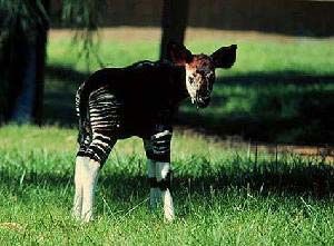
minaret (97.6%)         windsor chair (94.6%)            joshua tree (87.9%)                   okapi (87.8%)

  cougar body (27.6%)                beaver (27.5%)                    crocodile (25.0%)                      ant (25.0%)
Figure 5. Caltech-101 results. Top: some classes on which our method (L = 2, M = 200) achieved high performance. Bottom: some
classes on which our method performed poorly.

               Weak features           Strong features (200)
                                                                       it was not designed to cope with heavy clutter and pose
                                                                       changes. It is interesting to see how well our algorithm
  L      Single-level     Pyramid       Single-level   Pyramid         can do by exploiting the global scene cues that still remain
   0      15.5 ±0.9                      41.2 ±1.2                     under these conditions. Accordingly, our final set of ex-
   1      31.4 ±1.2      32.8 ±1.3       55.9 ±0.9    57.0 ±0.8        periments is on the Graz dataset [14] (Fig. 6), which is
   2      47.2 ±1.1      49.3 ±1.4       63.6 ±0.9    64.6 ±0.8
                                                                       characterized by high intra-class variation. This dataset has
   3      52.2 ±0.8      54.0 ±1.1       60.3 ±0.9    64.6 ±0.7
Table 2. Classification results for the Caltech-101 database.          two object classes, bikes (373 images) and persons (460 im-
                                                                       ages), and a background class (270 images). The image res-
                                  class 1 mis-    class 2 mis-         olution is 640 × 480, and the range of scales and poses at
          class 1 / class 2       classified as   classified as        which exemplars are presented is very diverse, e.g., a “per-
                                  class 2         class 1              son” image may show a pedestrian in the distance, a side
         ketch / schooner            21.6            14.8              view of a complete body, or just a closeup of a head. For this
         lotus / water lily          15.3            20.0              database, we perform two-class detection (object vs. back-
    crocodile / crocodile head       10.5            10.0              ground) using an experimental setup consistent with that of
         crayfish / lobster          11.3              9.1
                                                                       Opelt et al. [14]. Namely, we train detectors for persons and
          flamingo / ibis              9.5           10.4
Table 3. Top five confusions for our method (L    = 2, M = 200)
                                                                       bikes on 100 positive and 100 negative images (of which 50
on the Caltech-101 database.                                           are drawn from the other object class and 50 from the back-
                                                                       ground), and test on a similarly distributed set. We generate
                                                                       ROC curves by thresholding raw SVM output, and report
 Class         L=0            L=2       Opelt [14]   Zhang [25]
                                                                       the ROC equal error rate averaged over ten runs.
 Bikes      82.4 ±2.0 86.3 ±2.5         86.5          92.0                 Table 4 summarizes our results for strong features with
 People     79.5 ±2.3 82.3 ±3.1         80.8          88.0             M = 200. Note that the standard deviation is quite high be-
Table 4. Results of our method (M = 200) for the Graz database         cause the images in the database vary greatly in their level
and comparison with two existing methods.                              of difficulty, so the performance for any single run is depen-
                                                                       dent on the composition of the training set (in particular, for
(like crocodile), or “thin” objects (like ant). Table 3 shows          L = 2, the performance for bikes ranges from 81% to 91%).
the top five of our method’s confusions, all of which are              For this database, the improvement from L = 0 to L = 2
between closely related classes.                                       is relatively small. This makes intuitive sense: when a class
    To summarize, our method has outperformed both state-              is characterized by high geometric variability, it is difficult
of-the-art orderless methods [7, 25] and methods based on              to find useful global features. Despite this disadvantage of
precise geometric correspondence [1]. Significantly, all               our method, we still achieve results very close to those of
these methods rely on sparse features (interest points or              Opelt et al. [14], who use a sparse, locally invariant feature
sparsely sampled edge points). However, because of the                 representation. In the future, we plan to combine spatial
geometric stability and lack of clutter of Caltech-101, dense          pyramids with invariant features for improved robustness
features combined with global spatial relations seem to cap-           against geometric changes.
ture more discriminative information about the objects.
                                                                       6. Discussion
5.3. The Graz Dataset
                                                                          This paper has presented a “holistic” approach for image
   As seen from Sections 5.1 and 5.2, our proposed ap-                 categorization based on a modification of pyramid match
proach does very well on global scene classification tasks,            kernels [7]. Our method, which works by repeatedly sub-
or on object recognition tasks in the absence of clutter with          dividing an image and computing histograms of image fea-
most of the objects assuming “canonical” poses. However,               tures over the resulting subregions, has shown promising re-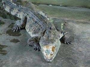
bike                                    person                                   background
                                                    Figure 6. The Graz database.

sults on three large-scale, diverse datasets. Despite the sim-       [10] J. Koenderink and A. V. Doorn. The structure of locally or-
plicity of our method, and despite the fact that it works not             derless images. IJCV, 31(2/3):159–168, 1999.
by constructing explicit object models, but by using global          [11] S. Lazebnik, C. Schmid, and J. Ponce. A maximum entropy
cues as indirect evidence about the presence of an object,                framework for part-based texture and object recognition. In
it consistently achieves an improvement over an orderless                 Proc. ICCV, 2005.
image representation. This is not a trivial accomplishment,          [12] D. Lowe. Towards a computational model for object recogni-
                                                                          tion in IT cortex. In Biologically Motivated Computer Vision,
given that a well-designed bag-of-features method can out-
                                                                          pages 20–31, 2000.
perform more sophisticated approaches based on parts and
                                                                     [13] A. Oliva and A. Torralba. Modeling the shape of the scene:
relations [25]. Our results also underscore the surprising                a holistic representation of the spatial envelope. IJCV,
and ubiquitous power of global scene statistics: even in                  42(3):145–175, 2001.
highly variable datasets, such as Graz, they can still provide       [14] A. Opelt, M. Fussenegger, A. Pinz, and P. Auer. Weak
useful discriminative information. It is important to develop             hypotheses and boosting for generic object detection and
methods that take full advantage of this information — ei-                recognition. In Proc. ECCV, volume 2, pages 71–84, 2004.
ther as stand-alone scene categorizers, as “context” mod-                 http://www.emt.tugraz.at/˜pinz/data.
ules within larger object recognition systems, or as tools for       [15] P. Quelhas, F. Monay, J.-M. Odobez, D. Gatica, T. Tuyte-
evaluating biases present in newly collected datasets.                    laars, and L. V. Gool. Modeling scenes with local descriptors
                                                                          and latent aspects. In Proc. ICCV, 2005.
Acknowledgments. This research was partially supported               [16] B. Schiele and J. Crowley. Recognition without correspon-
by the National Science Foundation under grants IIS-                      dence using multidimensional receptive field histograms.
0308087 and IIS-0535152, and the UIUC/CNRS/INRIA                          IJCV, 36(1):31–50, 2000.
collaboration agreement.                                             [17] J. Sivic, B. Russell, A. Efros, A. Zisserman, and W. Freeman.
                                                                          Discovering objects and their location in images. In Proc.
References                                                                ICCV, 2005.
                                                                     [18] D. Squire, W. Muller, H. Muller, and J. Raki. Content-based
 [1] A. Berg, T. Berg, and J. Malik. Shape matching and object            query of of image databases, inspirations from text retrieval:
     recognition using low distortion correspondences. In Proc.           inverted files, frequency-based weights and relevance feed-
     CVPR, volume 1, pages 26–33, 2005.                                   back. In Proceedings of the 11th Scandinavian conference
 [2] D. Blei, A. Ng, and M. Jordan. Latent Dirichlet allocation.          on image analysis, pages 143–149, 1999.
     Journal of Machine Learning Research, 3:993–1022, 2003.         [19] M. Swain and D. Ballard. Color indexing. IJCV, 7(1):11–32,
 [3] L. Fei-Fei, R. Fergus, and P. Perona. Learning generative            1991.
     visual models from few training examples: an incremental        [20] M. Szummer and R. Picard. Indoor-outdoor image classifi-
     Bayesian approach tested on 101 object categories. In IEEE           cation. In IEEE International Workshop on Content-Based
     CVPR Workshop on Generative-Model Based Vision, 2004.                Access of Image and Video Databases, pages 42–51, 1998.
     http://www.vision.caltech.edu/Image Datasets/Caltech101.        [21] A. Torralba, K. P. Murphy, W. T. Freeman, and M. A. Rubin.
 [4] L. Fei-Fei and P. Perona. A Bayesian hierarchical model for          Context-based vision system for place and object recogni-
     learning natural scene categories. In Proc. CVPR, 2005.              tion. In Proc. ICCV, 2003.
 [5] R. Fergus, P. Perona, and A. Zisserman. Object class recog-     [22] C. Wallraven, B. Caputo, and A. Graf. Recognition with
     nition by unsupervised scale-invariant learning. In Proc.            local features: the kernel recipe. In Proc. ICCV, volume 1,
     CVPR, volume 2, pages 264–271, 2003.                                 pages 257–264, 2003.
 [6] M. Gorkani and R. Picard. Texture orientation for sorting       [23] J. Willamowski, D. Arregui, G. Csurka, C. R. Dance, and
     photos “at a glance”. In IAPR International Conference on            L. Fan. Categorizing nine visual classes using local appear-
     Pattern Recognition, volume 1, pages 459–464, 1994.                  ance descriptors. In ICPR Workshop on Learning for Adapt-
 [7] K. Grauman and T. Darrell. Pyramid match kernels: Dis-               able Visual Systems, 2004.
     criminative classification with sets of image features. In      [24] H. Zhang, A. Berg, M. Maire, and J. Malik. SVM-KNN:
     Proc. ICCV, 2005.                                                    Discriminative nearest neighbor classification for visual cat-
                                                                          egory recognition. In Proc. CVPR, 2006.
 [8] E. Hadjidemetriou, M. Grossberg, and S. Nayar. Multireso-
                                                                     [25] J. Zhang, M. Marszalek, S. Lazebnik, and C. Schmid. Local
     lution histograms and their use in recognition. IEEE Trans.
                                                                          features and kernels for classifcation of texture and object
     PAMI, 26(7):831–847, 2004.
                                                                          categories: An in-depth study. Technical Report RR-5737,
 [9] T. Hofmann. Unsupervised learning by probabilistic latent
                                                                          INRIA Rhône-Alpes, 2005.
     semantic analysis. Machine Learning, 42(1):177–196, 2001.

You can also read