Techical report - Italian Journal of ...
←
→
Page content transcription
If your browser does not render page correctly, please read the page content below
DOI: 10.7343/as-2021-499 Techical report
Assessing the long-term sustainability of the groundwater resources
in the Bacchiglione basin (Veneto, Italy) with the Mann–Kendall test:
suggestions for higher reliability
Valutazione della sostenibilità a lungo termine della risorsa idrica sotterranea nel bacino del
Bacchiglione (Veneto, Italia) con il test di Mann–Kendall: suggerimenti per una maggiore
affidabilità
Mara Meggiorin, Giulia Passadore, Silvia Bertoldo, Andrea Sottani, Andrea Rinaldo
Riassunto: Il sistema acquifero all’interno del bacino del leggermente diverso: 2000-2014. Il presente studio investiga le
Bacchiglione (Veneto, IT) è di notevole importanza sociale, ragioni di tale divergenza nelle risultanze concentrandosi sulla
economica ed ecologica ma, circa la sostenibilità del suo utilizzo, sensibilità del metodo rispetto al periodo di tempo considerato.
vi sono risultati discordanti tra i precedenti studi. Questo studio Dopo aver effettuato un’analisi di Fourier sulla serie temporale
indaga quindi la sostenibilità quantitativa a lungo termine di tale più lunga disponibile, per la valutazione dello stato quantitativo
sistema idrico sotterraneo applicando una metodologia statistica del corpo idrico questo lavoro suggerisce di applicare il test di
che può essere utilizzata in studi similari. In particolare, le serie Mann-Kendall a serie temporali più lunghe di 20 anni, altrimenti
temporali disponibili vengono analizzate con i test di Mann- affette dalle lunghe periodicità interannuali del ciclo idrologico.
Kendall e di Sen’s slope, due analisi robuste e già ampiamente Un’ulteriore analisi di due serie temporali mensili della durata
utilizzate negli studi ambientali. L’analisi è condotta su un dataset di 60 anni, riferite al periodo tra 1960 e il 2020, suggerisce la
ampio ed eterogeneo che raccoglie serie temporali orarie del livello sostenibilità dell’attuale utilizzo della risorsa idrica sotterranea
delle acque sotterranee in 79 punti di controllo, registrate nel anche se il sistema nel passato è stato di fatto depauperato. I
periodo 2005-2019. Il test identifica trend decrescenti significativi risultati dimostrano quindi che è possibile ottenere risultati più
per la maggior parte dei record disponibili, differentemente affidabili e conclusioni significative sulla sostenibilità a lungo
da precedenti studi sullo stato quantitativo della risorsa che termine del sistema idrico sotterraneo
coprivano il dominio qui indagato in un periodo di tempo
Keywords: seasonal Mann-Kendall test, Sen’s slope estimator, Abstract: The social, economic, and ecological importance of the
sustainability, groundwater level, Bacchiglione. aquifer system within the Bacchiglione basin (Veneto, IT) is noteworthy,
and there is considerable disagreement among previous studies over its
Parole chiave: test stagionale Mann-Kendall, test Sen’s Slope, sustainable use. Investigating the long-term quantitative sustainability
sostenibilità, livello delle acque sotterranee, Bacchiglione.
of the groundwater system, this study presents a statistical methodology
that can be applied to similar cases. Using a combination of robust and
Mara Meggiorin widely used techniques, we apply the seasonal Mann–Kendall test and
Silvia Bertoldo, Andrea Sottani the Sen’s slope estimator to the recorded groundwater level timeseries.
Sinergeo Srl – Vicenza, Italy The analysis is carried out on a large and heterogeneous proprietary
mara.meggiorin@dicea.unipd.it dataset gathering hourly groundwater level timeseries at 79 control
sbertoldo@sinergeo.it
asottani@sinergeo.it points, acquired during the period 2005–2019. The test identifies
significant decreasing trends for most of the available records, unlike
Giulia Passadore previous studies on the quantitative status of the same resource which
Dipartimento di Ingegneria Civile, Edile e Ambientale, Università di Padova
giulia.passadore@dicea.unipd.it
covered the domain investigated here for a slightly different period:
2000–2014. The present study questions the reason for such diverging
Andrea Rinaldo results by focusing on the method’s accuracy. After carrying out a Fourier
Dipartimento di Ingegneria Civile, Edile e Ambientale, Università di Padova analysis on the longest available timeseries, for studies of groundwater
Laboratory of Echohydrology (ECHO/IIE/ENAC), École Polytechnique
Fédérale de Lausanne, Switzerland status assessment this work suggests applying the Mann–Kendall test to
andrea.rinaldo@epfl.ch timeseries longer than 20 years (because otherwise the analysis would
be affected by interannual periodicities of the water cycle). A further
Ricevuto/Received: 15 February 2021 - Accettato/Accepted: 16 March 2021 analysis of two 60-year-long monthly timeseries between 1960 and
Pubblicato online/Published online: 30 March 2021 2020 supports the actual sustainable use of the groundwater resource,
This is an open access article under the CC BY-NC-ND license: the past deployment of the groundwater resources notwithstanding.
http://creativecommons.org/licenses/by-nc-nd/4.0/ Results thus prove more reliable, and meaningful inferences on the long-
© Associazione Acque Sotterranee 2021 term sustainability of the groundwater system are possible.
Acque Sotterranee - Italian Journal of Groundwater (2021) - AS36 - 499: 35 - 48 35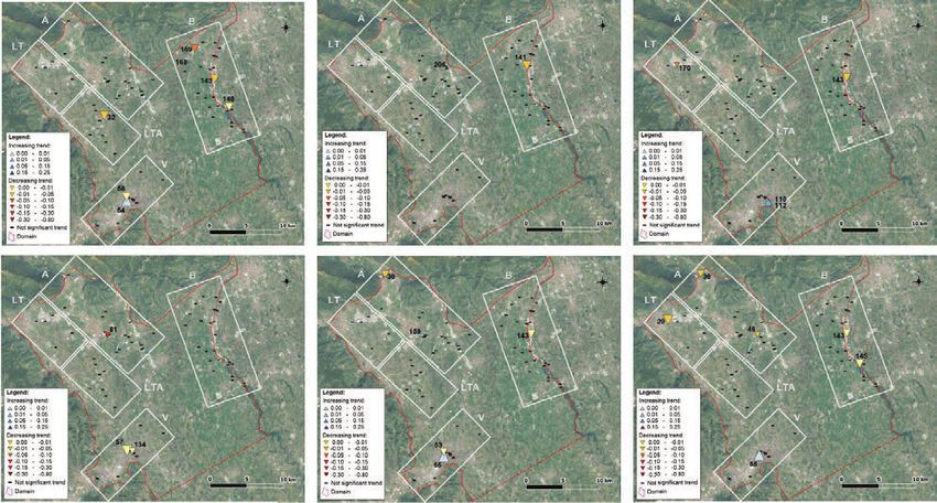
DOI: 10.7343/as-2021-499

Introduction                                                       parameters: from most common analyses of temperature and
   In the past, groundwater resources played a major role          precipitations (Gan 1995; Wibig and Glowicki 2002; Mondal
in economic and human development worldwide and now                et al. 2012), to most peculiar studies on number of wet and
numerous aquifer systems have begun to show the effects            dry months (Zhang et al. 2009), evapotranspiration (Tabari
of overexploitation or pollution events. One example is the        et al. 2011; Shadmani et al. 2012), atmospheric deposition
central area of the Veneto Region, which has always been           (Drápela and Drápelová 2011; Waldner et al. 2014), hail
characterized by an abundance of groundwater resources:            (Gavrilov et al. 2010) and aridity (Some’e et al. 2013; Hrnjak
the drinking water supply system is mainly supplied by             et al. 2014). Specifically on hydrological timeseries, many
groundwater and, owing to this abundance of good-quality           studies tested stream flows all over the world (Douglas et al.
water, both industrial and agricultural activities have            2000; Kahya and Kalaycı 2004; Svensson et al. 2005), few
developed in this area with high demands for water. Due            focused on groundwater levels (Panda et al. 2007; Polemio
to the importance of this aquifer system, many studies have        and Casarano 2008; Du Bui et al. 2012; Tabari et al. 2012;
investigated it extensively due to a concern about the possible    Vousoughi et al. 2013; Patle et al. 2015; Ribeiro et al. 2015)
overexploitation of the resource coupled with the climate          and still less on groundwater quality (Ribeiro and Macedo
change affecting the local water balance. Between those            1995; Daughney and Reeves 2006; Aguilar et al. 2007;
studies, Passadore et al. (2012) notices a lowering of the water   Wahlin and Grimvall 2010).
table, while ARPAV (2016) observes a rise in the monitored            Other than the sustainability assessment of the groundwater
groundwater level.                                                 system, this study highlights a critical aspect of the application
   Following the definition of the Italian law (Legislative        of the Mann–Kendall test and the Sen’s slope estimator that
Decree no. 30 of 16.03.2009), the assessment of the                is linked to the period analysed. Indeed, the results of the
quantitative status of a groundwater system is based on an         dataset used here differ depending on the period considered.
analysis of the groundwater level. Specifically, as explained      Moreover, the results are opposite to those of ARPAV (2016),
and applied in ARPAV (2016), the trend in the groundwater          which carried out the same analysis in the Veneto Region,
level over time, showing aquifers storage and emptying, is         including a few timeseries recorded at control points within
an effective indicator of the exploitation sustainability of       the Bacchiglione basin. Thus, this study aims to better
groundwater systems. Anthropogenic and climatic effects            understand the methodological approach, with the intention
on the water balance are not differentiated; the quantitative      to use the method properly and deliver more reliable results.
status of the groundwater resource is assessed by looking          First, the Mann–Kendall test and the Sen’s slope estimator are
at the overall depletion or stability of the resource volume.      applied to the available dataset to evaluate groundwater level
Thus, if the evaluated trend for a specific groundwater            trends between 2005 and 2019, and to test the applicability
system is positive or stationary, the quantitative status of the   of the trend testing procedure for groundwater level datasets
water body is assessed as good. Following this line, ARPAV         that are usually characterised by missing data and timeseries
(2016) observes upward timeseries trends and assesses the          of different lengths. Then, diverging results are further
groundwater system as having a good quantitative status,           investigated because the results arise a critical aspect of the
while Passadore et al. (2012) notices downward trends.             method in assessing long-term groundwater trends, and
   Due to such opposite results, this study assesses the           finally, a few clear suggestions are presented for achieving
quantitative status of the groundwater resource by detecting       more reliable conclusions from assessing the sustainable
trends in the groundwater level at several control points          exploitation of groundwater systems that respond slowly to
within the Bacchiglione basin. The Mann–Kendall (MK) test          human and hydraulic stresses.
(Mann 1945; Kendall 1948) and the Sen’s slope estimator (Sen
1968) are used to evaluate the significance and magnitude          Study area
of the trends. Such a method combination is widely used in           The trend detection analysis is applied to several control
many environmental fields, as it is often interesting to detect    points that continuously measure the groundwater level
any possible statistically significant increasing or decreasing    within the basin of the Bacchiglione river located in the
trends as a first indicator of human or climate change             Veneto plain and covering the alluvial plain to the north of
effects. Trend testing aims to determine in statistical terms      Vicenza, the study domain is shown in Figure 1. Abundant
if a random variable has generally increasing or decreasing        groundwater is present here, owing to two main factors: the
values (Helsel and Hirsch 2002). Two main trend tests exist:       particularly permeable subsoil and the strong connections
parametric tests, which require independent and normally           between rivers and groundwater that ensure the recharging
distributed data, and non-parametric tests, which simply           of the aquifer system.
need independent data. Often the choice goes to the Mann–            Geologically speaking, in the upper plain, the Piedmont
Kendall test for its simplicity and robustness. Indeed, it can     area has a continuous, undifferentiated gravelled subsoil
be applied even in the presence of missing values or measures      because of the overlapping alluvial fans. Such overlapping is
below the detection limit, which is quite common in                due to the instability of rivers and their wide movement in
environmental issues (Gavrilov et al. 2016). Therefore, it has     past centuries. Going downstream towards South-East, the
been largely used for analysing trends in several climatologic     course material thickness decreases gradually in the middle

36                                                                 Acque Sotterranee - Italian Journal of Groundwater (2021) - AS36 - 499: 35 - 48
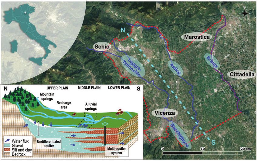
DOI: 10.7343/as-2021-499

                          Fig. 1 - Plan view of the study area with main cities, main river tracks and the reference geological scheme of the Veneto plain.
Fig. 1 - Vista in pianta dell’area di studio con riportate le città principali, i fiumi più importanti nel territorio e lo schema geologico di riferimento della pianura veneta.

plain to the point where the coarse layers vanish into fine                               the installed sensors continuously recorded the hydraulic
materials in the lower plain (Dal Prà et al. 1976, 1977). At                              head, but they were installed during different periods, thus
this point, gravelled layers of alluvial fans are rare, relatively                        the available timeseries have a variable length ranging from
thin, and deep. This Quaternary formation lies on a bedrock                               3 months to almost 14 years. In addition, timeseries can have
of the Tertiary age located at a depth ranging from a few                                 gaps due to the breakdown of sensors or due to particularly
meters in the upper Veneto plain to several hundred meters                                dry periods for which the specific sensor is not located deep
towards the southeast.                                                                    enough or the well depth is insufficient. Moreover, there may
   The hydrogeological system is connected with the local                                 be some outliers due to sensor malfunctions or to the pumping
geological characteristics. Thus, in the Piedmont area,                                   effect of nearby wells, and these outliers must be removed
there exists a unique powerful unconfined aquifer that lies                               for the purpose of this study. Outliers are usually defined as
directly on the bedrock and has a water table that oscillates                             values below the 10th and above the 90th percentiles, which
freely depending on periodic hydraulic dynamics. In the                                   are easily identifiable in timeseries data depicted in a boxplot
middle plain, the Quaternary formation is stratified, which                               graph. However, some outliers could be representative of
determines the presence of a layered multi-aquifer system.                                hydrologically relevant peaks, therefore they are meaningful
Given its ease of water extraction and its protection from                                values. For this reason, series with identified outliers in the
surface polluting events, the multi-aquifer system is the main                            boxplot are checked by displaying values against time to
water resource for the public supply of drinkable water in the                            classify outliers as natural phenomena or measurement errors.
area, mainly the 3rd and 4th confined aquifers.                                           To carry out a meaningful analysis, records were then selected
                                                                                          that had at least two years of data and less than 50% of values
Data and methods                                                                          missing, thus 79 sensors were selected (listed in Table 1).
  Owing to the instruments and proprietary databases of                                      As a trend test, this study applies the widely used MK
Sinergeo, the present study is based on a large amount of                                 test, a non-parametric test assuming stable, independent,
data, which is heterogeneous in time and space. Within the                                and random timeseries with equal probability distributions.
domain of interest, 102 monitoring points were equipped with                              Unlike parametric trend tests, there is no normality
automatic instrumentation to record the piezometric head                                  assumption, and the MK test is less affected by outliers or
with a sampling interval of 1 or 3 hours. However, as happens                             missing data than the linear regression method (Ribeiro et
in many real case studies, the available dataset is affected by                           al. 2015). Yue et al. (2002) found that the test becomes more
missing values and outliers. Missing data occurred because                                powerful the greater the absolute magnitude of the trend and

Acque Sotterranee - Italian Journal of Groundwater (2021) - AS36 - 499: 35 - 48                                                                                           37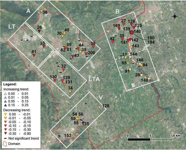
DOI: 10.7343/as-2021-499

Tab. 1 - List of the sensors considered for the timeseries analysis with the Mann-Kendall test and the Sen’s slope estimator: recorded period, timeseries length [years], percentage of
missing data [%], intercepted aquifer type, depth of the piezometer [m], average depth of the water table [m].
Tab. 1 - Elenco dei sensori utilizzati per l’analisi delle serie storiche con i test Mann-Kendall e Sen’s Slope: periodo monitorato, lunghezza della serie [anni],
percentuale di dati mancanti [%], acquifero intercettato, profondità del piezometro [m], profondità media del livello di falda [m].

      ID           Recorded period               Series length           % Missing data             Aquifer type               Piezometer                Average depth of
                                                                                                                                  depth                   the water table
 2                apr 15 - mar 18                        2.9                      1.4                 unconfined                   35.0                        18.6
 25               apr 06 - oct 17                       11.5                      3.8                 unconfined                   29.0                        20.3
 26               jul 06 - oct 18                       12.2                      7.9                 unconfined                  123.0                        95.9
 27               jun 07 - nov 18                       11.5                     15.0                 unconfined                   30.2                        25.5
 28               jul 06 - feb 18                       11.6                      0.0                 unconfined                    6.0                         4.8
 29               aug 06 - dec 18                       12.4                     18.5                 unconfined                   15.8                        14.4
 30               jan 08 - dec 18                       11.0                     14.8                 unconfined                   29.4                        27.1
 31               jul 06 - jan 19                       12.5                      0.0                 unconfined                   11.5                         8.0
 32               jul 07 - dec 18                       11.5                      4.7                 unconfined                   21.2                        16.5
 33               may 05 - dec 18                       13.6                      4.2                 unconfined                  104.0                        74.6
 34               jul 06 - nov 18                       12.4                      0.0                 unconfined                    6.0                         2.0
 35               jul 06 - nov 18                       12.4                      2.5                 unconfined                   22.0                        14.2
 36               mar 09 - jul 18                        9.3                      0.0                 unconfined                   22.8                        10.7
 37               jul 06 - dec 18                       12.4                      0.1                 unconfined                   27.0                        24.3
 38               jul 06 - nov 18                       12.4                     10.4                 unconfined                   33.6                        28.8
 39               aug 07 - dec 18                       11.4                     15.1                 unconfined                   34.8                        29.8
 40               jul 06 - dec 18                       12.4                      2.8                 unconfined                    8.5                         5.9
 41               nov 07 - dec 18                       11.1                     25.2                 unconfined                   65.9                        46.4
 42               apr 07 - aug 18                       11.3                      5.0                 unconfined                   17.3                        12.1
 43               apr 10 - jan 19                        8.7                      1.2                 unconfined                     -                         27.1
 44               apr 10 - nov 18                        8.6                      2.2                 unconfined                   66.5                        34.8
 45               oct 15 - nov 18                        3.0                      0.0                 unconfined                   18.0                         5.9
 46               mar 12 - nov 18                        6.7                      4.0                 unconfined                   45.5                        26.4
 53               may 05 - aug 13                        8.3                      3.6                  confined                    41.5                         3.3
 54               jun 05 - dec 18                       13.6                     18.9                  confined                    60.0                         2.5
 55               jun 05 - dec 18                       13.5                     20.6                  confined                   101.0                         1.4
 56               jun 05 - dec 17                       12.5                     24.0                  confined                    96.5                         3.2
 57               apr 05 - dec 18                       13.7                      0.1                 unconfined                    9.7                         2.0
 58               may 08 - feb 19                       10.8                     10.7                 unconfined                    7.5                        2.8
 59               may 08 - feb 19                       10.8                     29.9                 unconfined                    6.4                         1.9
 80               nov 13 - dec 18                        5.1                      1.2                 unconfined                   55.0                        38.6
 81               nov 13 - dec 18                        5.1                      0.0                 unconfined                   60.0                        50.0
 82               oct 11 - nov 18                        7.1                      0.2                 unconfined                   65.0                        53.0
 83               oct 11 - nov 16                        5.1                      1.8                  confined                      -                         25.9
 91               sep 11 - nov 18                        7.2                      0.6                 unconfined                   26.0                         2.9
 92               oct 11 - nov 18                        7.2                     22.7                 unconfined                     -                          5.4
 94               sep 11 - nov 18                        7.2                     13.0                 unconfined                   26.5                         2.3
 95               sep 11 - feb 19                        7.4                     12.6                 unconfined                   34.0                         4.6
 103              apr 10 - dec 18                        8.7                      0.2                 unconfined                    5.6                         1.8
 104              apr 10 - mar 17                        6.9                      2.1                  confined                      -                          2.7

38                                                                                           Acque Sotterranee - Italian Journal of Groundwater (2021) - AS36 - 499: 35 - 48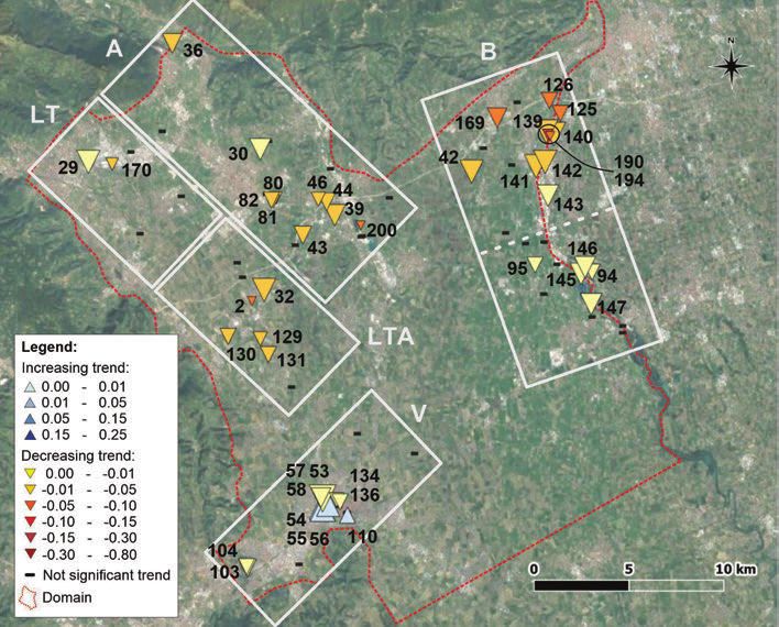
DOI: 10.7343/as-2021-499

Tab. 1 - List of the sensors considered for the timeseries analysis with the Mann-Kendall test and the Sen’s slope estimator: recorded period, timeseries length [years], percentage of
missing data [%], intercepted aquifer type, depth of the piezometer [m], average depth of the water table [m].
Tab. 1 - Elenco dei sensori utilizzati per l’analisi delle serie storiche con i test Mann-Kendall e Sen’s Slope: periodo monitorato, lunghezza della serie [anni],
percentuale di dati mancanti [%], acquifero intercettato, profondità del piezometro [m], profondità media del livello di falda [m].

       ID           Recorded period               Series length          % Missing data             Aquifer type                Piezometer                Average depth of
                                                                                                                                   depth                   the water table
  110              dec 10 - dec 18                       8.0                      10.2                 confined                     48.0                         6.7
  111              dec 10 - dec 18                       8.0                       3.3                 confined                     50.0                         3.6
  112              dec 10 - dec 18                        7.9                      2.1                 confined                     48.0                         6.4
  113              apr 15 - dec 18                        3.7                     12.0                 confined                     10.0                         6.2
  114              may 15 - dec 18                       3.6                      33.4                 confined                     42.5                         0.4
  125              oct 11 - feb 19                        7.4                      0.0                unconfined                    35.0                        22.5
  126              oct 11 - feb 19                        7.4                      0.0                unconfined                    35.0                        23.8
  128              nov 11 - feb 19                        7.2                     2.2                  confined                      8.0                         2.0
  129              feb 12 - feb 19                        7.0                     4.6                 unconfined                    12.0                         8.5
  130              feb 12 - feb 19                        7.0                      0.0                unconfined                    26.0                        12.7
  131              feb 12 - feb 19                        7.0                      0.0                unconfined                    12.0                         4.3
  133              apr 15 - dec 18                        3.7                     15.2                unconfined                    6.2                          2.5
  134              oct 11 - dec 18                        7.2                     11.8                unconfined                     6.0                         4.4
  135              oct 11 - dec 18                        7.2                      0.0                 confined                      6.0                         2.5
  136              oct 11 - dec 18                        7.2                      0.0                 confined                      6.0                         3.9
  139              mar 07 - nov 18                       11.7                      0.0                unconfined                    30.0                        16.4
  140              mar 07 - nov 18                       11.7                      2.5                unconfined                    25.0                        15.7
  141              mar 07 - nov 18                       11.7                      0.0                unconfined                    20.0                         6.4
  142              mar 07 - nov 18                       11.7                      0.0                unconfined                    22.0                         9.5
  143              may 08 - nov 18                       10.5                      0.0                unconfined                    20.0                         8.2
  144              may 08 - nov 18                       10.5                      0.0                unconfined                    20.0                         6.7
  145              may 08 - nov 18                       10.5                     0.8                 unconfined                    20.0                         5.9
  146              may 08 - nov 18                       10.5                      0.0                unconfined                    18.0                         6.7
  147              may 08 - nov 18                       10.5                      0.0                unconfined                    20.0                         7.6
  148              may 08 - nov 18                       10.5                      0.0                unconfined                    14.0                         3.4
  149              may 08 - nov 18                       10.5                      1.1                unconfined                    12.0                         2.0
  151              mar 07 - nov 18                       11.7                      0.0                unconfined                    25.0                        16.4
  153              oct 09 - oct 18                        9.0                      0.0                unconfined                     6.0                         2.1
  159              jul 13 - jul 18                        5.0                      0.0                unconfined                    60.0                        49.4
  168              jan 16 - jan 19                       3.0                       0.0                unconfined                    30.0                        19.6
  169              sep 09 - jan 19                        9.4                      2.1                unconfined                    35.0                        23.0
  170              mar 13 - jan 19                        5.9                      9.3                unconfined                    20.0                        16.8
  190              jun 14 - nov 18                       4.4                       9.9                unconfined                    25.0                        16.7
  194              jun 14 - nov 18                       4.4                      35.1                unconfined                    15.0                         9.7
  198              apr 15 - nov 18                       3.6                       1.0                unconfined                    40.0                        34.6
  200              nov 14 - feb 19                       4.2                      13.5                unconfined                    40.0                        26.7
  203              mar 15 - feb 19                        3.9                      0.0                unconfined                    37.0                        25.8
  204              oct 15 - mar 18                        2.5                      0.0                unconfined                      14.0                          12.0
  206              mar 15 - mar 19                        3.9                     12.4                unconfined                      24.6                          14.3

Acque Sotterranee - Italian Journal of Groundwater (2021) - AS36 - 499: 35 - 48                                                                                                  39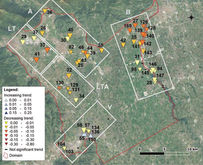
DOI: 10.7343/as-2021-499
as the sample size increases, while its power decreases if the where ni is the number of values in season i and p is the
amount of variation increases. Moreover, potential scaling number of seasons, i.e. 12 months for this case study. The
effects could be present in identifying timeseries trends, as so defined statistic Zk is then compared to the threshold
found in some runoff studies (Koutsoyiannis 2003; Hamed Zcrit defined as the value of the standard normal distribution
2008). The specific effect is not considered here, but scaling corresponding to an exceedance probability of α/2, Z(1-α/2).
is accounted by a modified MK test, which can eliminate The null hypothesis is rejected if |Zk| >Z(1-α/2), thus a
potential contradictions related to local or regional scales. significant trend in the timeseries is detected, otherwise the
The analysis consists of using Kendall’s significance test null hypothesis of no trend cannot be rejected.
for a time variable to detect the trend. In this test, two Sen’s slope estimator (Sen 1968) is a usual additional analysis
hypotheses are tested for each timeseries: the null hypothesis to the MK test because it estimates the trend slope for the
(H0) of no trend and the alternative hypothesis (Ha) of a variable Y over time t (Drápela and Drápelová 2011; Mondal
significant trend. As for all statistical hypothesis tests, Ha is et al. 2012; Gocic and Trajkovic 2013; Ribeiro et al. 2015;
accepted if there is an unlikely realization of H0 according Rahman and Dawood 2017). For each month k, in a sample
to a predefined threshold probability, the significance level of nk pairs of data yi,yj with 1≤j≤i≤nk, the slope estimate is the
a. Therefore, if the probability p is lower than the chosen a, median of Dijk:
the null hypothesis of no trend should be rejected and the
alternative hypothesis accepted, otherwise the null hypothesis yik − y jk
Dijk = for k=1,...,12
cannot be rejected. i− j
Specifically, the Kendall’s S statistic is used to understand
whether a variable Y tends to monotonically increase or The estimator is robust against outliers and serial correlation
decrease over time t. Precisely, for a timeseries (Y; t) composed effects are unlikely because, in this study, Dijk are computed
by n time steps, for instants i>j, all values pairs yi,yj are on values that are 12 months apart (Hirsch et al. 1982).
inspected and classified into yi>yj or yi 0
k data missing in the considered period: 77 sensors for the
Z = three-year analysis and 59 for the latter. Both periods were
K 0 if Sk = 0
S +1 selected to gather the most control points, and they occur to
k if Sk < 0 start from a period of maximum hydraulic head and end in
s k a dry period. Consequently, both analyses identify more than
60% of trends as significant, almost all negative, visible in
where sk is the standard deviation of Sk and it is calculated as Figures 2 and 3. For the ease of comparison, dataset sensors
are categorized into five different sectors depending on the
p
most likely hydraulic drivers: Leogra-Timonchio river system
ni
s=
k ∑ 18 ( n − 1)( 2n + 5)
i =1
i i
(LT), Astico river (A), both Leogra-Timonchio and Astico
influence (LTA), Brenta river (B) and in the downstream
confined system close by Vicenza (V).
40 Acque Sotterranee - Italian Journal of Groundwater (2021) - AS36 - 499: 35 - 48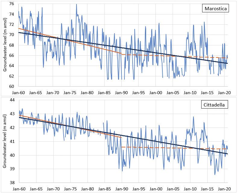
DOI: 10.7343/as-2021-499
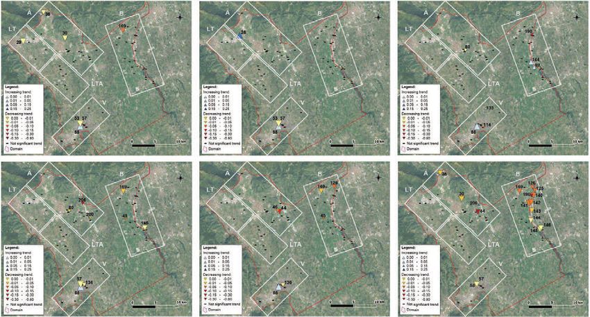
Fig. 2 - Statistically significant trends
of the groundwater level timeseries on
the period 2015-2017. The magnitude
of the decreasing or increasing trends
(symbol colour) is estimated by the Sen’s
slope estimator. Gray rectangles subdivide
the domain into five sectors depending on
main hydraulic drivers. Black numbers
show sensors ID.
Fig. 2 - Trend statisticamente
significativi del livello delle acque
sotterranee, nel periodo 2015-2017.
L’entità dei trend decrescenti o
crescenti (rappresentata dalla classe di
colore) è stata valutata con il test Sen’s
Slope. I rettangoli grigi suddividono
il dominio in cinque settori a seconda
dei drivers idraulici. I numeri in nero
riportano gli ID dei sensori.
Fig. 3 - Statistically significant trends
of the groundwater level timeseries on
the period 2009-2018. The magnitude
of the decreasing or increasing trends
(symbol colour) is estimated by the Sen’s
slope estimator. Gray rectangles subdivide
the domain into five sectors depending on
main hydraulic drivers. Black numbers
show sensors ID.
Fig. 3 - Trend statisticamente
significativi del livello delle acque
sotterranee, nel periodo 2009-2018.
L’entità dei trend decrescenti o
crescenti (rappresentata dalla classe di
colore) è stata valutata con il test Sen’s
Slope. I rettangoli grigi suddividono
il dominio in cinque settori a seconda
dei drivers idraulici. I numeri in nero
riportano gli ID dei sensori.
To avoid bias linked to the selected period, the third Figure 4 reports identified significant overall trends with
analysis does not define the period, and all available symbol sizes dependent on the timeseries length, highlighting
timeseries were analysed, even if they have different longer records.
recording lengths. As a reminder of the dataset heterogeneity, Results are slightly different from previous period-defined
Acque Sotterranee - Italian Journal of Groundwater (2021) - AS36 - 499: 35 - 48 41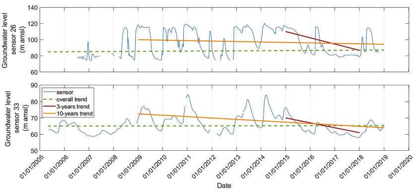
DOI: 10.7343/as-2021-499

                                                                                                                                         Fig. 4 - Statistically significant trends
                                                                                                                                         of the groundwater level timeseries,
                                                                                                                                         considering all available timeseries. The
                                                                                                                                         magnitude of the decreasing or increasing
                                                                                                                                         trends (symbol colour) is estimated by the
                                                                                                                                         Sen’s slope estimator. Gray rectangles
                                                                                                                                         subdivide the domain into five sectors
                                                                                                                                         depending on hydraulic drivers. Black
                                                                                                                                         numbers show sensors ID.

                                                                                                                                         Fig. 4 - Trend statisticamente
                                                                                                                                         significativi del livello delle acque
                                                                                                                                         sotterranee, considerando l’intero
                                                                                                                                         periodo disponibile. L’entità dei trend
                                                                                                                                         decrescenti o crescenti (rappresentata
                                                                                                                                         dalla classe di colore) è stata valutata
                                                                                                                                         con il test Sen’s Slope. I rettangoli
                                                                                                                                         grigi suddividono il dominio in
                                                                                                                                         cinque settori a seconda dei drivers
                                                                                                                                         idraulici. I numeri in nero riportano
                                                                                                                                         gli ID dei sensori.

analyses: note that sensors 26 and 33 do not show significant                              the different periods considered, with continuous lines if they
trends for the all-inclusive analysis, but they do show a                                  have been defined as statistically significant by the MK test or
decreasing trend in the two previous analyses with 3- and 10-                              with dashed lines otherwise.
year periods. This discrepancy is due to their recording start                               Nevertheless, even in this all-inclusive test, the majority of
time, which was spring 2005. Indeed, this antecedent period                                identified significant trends are negative. The only exceptions
between 2005 and 2009 was characterized by a generally low                                 are the four sensors with a positive average trend slope of 3.3
hydraulic head with a particularly dry period in spring and                                mm/month: all are in the confined system of the Vicenza
summer 2007. This low water table period clearly influences                                area. Other shallower sensors nearby show decreasing trends
the Mann–Kendall test and the Sen’s slope estimator: as an                                 instead: they mostly intercept the phreatic aquifer. There is
example, Figure 5 highlights the distinct estimated trends for                             only one (sensor 136) with a decreasing trend that intercepts

Fig. 5 - Groundwater level timeseries of sensors 26, 33 and statistically significant trends. Trends are estimated for three different time periods: all recording, 2015-2017, 2009-
2018. Trend lines are continuous if the trend has been evaluated as significant, dashed otherwise.
Fig. 5 - Serie storiche del livello delle acque sotterranee dei sensori 26, 33 ed i loro trend. I trend delle serie storiche sono stimati per i tre differenti periodi
considerati: l’intera serie disponibile, 2015-2017, 2009-2018. Le linee di tendenza sono continue se il trend è stato valutato significativo, tratteggiato altrimenti.

42                                                                                         Acque Sotterranee - Italian Journal of Groundwater (2021) - AS36 - 499: 35 - 48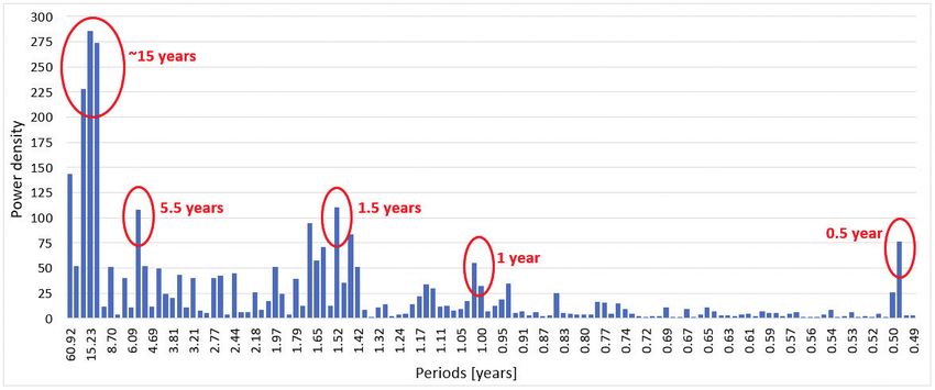
DOI: 10.7343/as-2021-499

Tab. 2 - Summary of the Mann-Kendall test and Sen’s slope estimator for the seasonal (monthly MK), the overall, the 3-years and 10-years analyses: number of analysed sensors, identified
statistically significant positive and negative trends, not significant trends, their percentages and the mean significant positive and negative slopes for the whole dataset [cm/month].
Tab. 2 - Riassunto dei risultati del test Mann-Kendall test e del Sen’s slope per le analisi stagionale (MK mensile) e considerando l’intera serie storica, 3 anni e 10
anni: il numero di serie storiche analizzate, i trend valutati statisticamente positivi e negativi, trend non significativi, le loro percentuali e la pendenza media dei
trend statisticamente positivi e negativi per l’intero dataset disponibile [cm/mese].

                                                                                N. not                                             % not
                                           N. pos            N. neg                                % pos          % neg                             Average pos          Average
                       N. sensors                                             significant                                        significant
                                           trends            trends                                trends         trends                               slope            neg slope
                                                                                trends                                             trends
 Jan MK                     79                2                  5                 72                3%             6%               91%                 2.49              -2.81
 Feb MK                     79                1                  1                 77                1%             1%               97%                22.86              -4.44
 Mar MK                     79                2                  2                 75                3%             3%               95%                 1.12              -4.41
 Apr MK                     79                0                  3                 76               0%              4%               96%                   -               -4.75
 May MK                     79                2                  3                 74                3%             4%               94%                 1.03              -1.28
 Jun MK                     79                1                  5                 73                1%             6%               92%                 0.46              -1.16
 Jul MK                     79                1                  6                 72                1%             8%               91%                 0.40              -1.52
 Aug MK                     79                2                  2                 75                3%             3%               95%                 3.08              -1.01
 Sept MK                    79                4                  3                 72                5%             4%               91%                 0.38              -5.59
 Oct MK                     79                1                  8                 70                1%             10%              89%                 0.29              -4.77
 Nov MK                     79                1                  6                 72                1%             8%               91%                 0.42              -6.55
 Dec MK                     79                1                 16                 62                1%             20%              78%                14.91              -5.92
 Overall MK                 79                4                 41                 34                5%             52%              43%                 0.33              -2.82
 MK 3years                  77                1                 47                 29                1%             61%              38%                 0.21             -10.19
 MK 10years                 59                2                 45                 12                3%             76%              20%                 0.15              -2.98

the first confined aquifer, but it is close to a few pumping                                  flowrates (listed in Table 3), both 13 years long and recorded
wells, and it is probably affected by them. Negative slopes                                   by ARPAV stations. The flowrate timeseries of the Leogra river
are indeed present in the confined system for the shallowest                                  was made available by the CIN [Centro Idrico di Novoledo,
aquifer, although their magnitude is less than the decreasing                                 personal communication (2019)] for the monitoring station in
trends of the upstream unconfined aquifer within the river                                    Torrebelvicino.
systems of Leogra-Timonchio, Astico, and Brenta. With the                                        They do not generally observe significant trends:
shortest timeseries usually characterized by highest negative                                 precipitation sometimes shows significant seasonal trends,
slopes removed, the average decreasing slope for the domain                                   while rivers timeseries do show overall significant trends
is 2.13 cm/month, whereas Table 2 summarizes the results for                                  for the periods 2015–2017 and 2009–2018. Specifically, in
the whole dataset.                                                                            the Brenta area, four rainfall timeseries have a decreasing
   To highlight the possible trend patterns depending on                                      seasonal trend between August and September, but for the
balance factors with specific seasonal trends, the seasonal                                   groundwater timeseries, if they have a trend, it is upward.
MK tests the trend significance for each month considering                                    This discrepancy could be due to irrigation, which is quite
the whole timeseries available. Observing resulting trends                                    a diffuse practice in this area, and which balances the
in Table 2, Figures 6 and 7, all months show no significant                                   precipitation deficit. The last significant rainfall seasonal
trends for the majority of sensors; those sensors with                                        trend is positive and is seen in January for the weather
seasonally significant trends vary depending on the month.                                    station in Montecchio Precalcino, likely influencing the A
A few similarities are present between the different river                                    and LTA sectors. However, neither sectors see any significant
systems: decreasing trends in June and July for the Leogra-                                   January trend except for one decreasing trend. Precipitation
Timonchio, Astico, and Brenta sectors, and dramatically                                       trends are therefore not relatable to those of the water table.
decreasing trends in December for the two latter sectors. The                                 The Astico and Brenta river flowrate timeseries do present
sector around the Brenta river is the one most visibly affected                               significant overall decreasing trends for the 3- and 10-year
by negative trends: 16 decreasing trends in the winter month                                  analyses, but they do not for the all-inclusive analysis. These
of December, while other months have between one and three                                    river decreasing trends are in line with those of surrounding
identified decreasing trends.                                                                 sensors, but they are not sufficient evidence to deduce more
   To relate the identified trends with trends related to water                               about their hydraulic connections. The Leogra-Timonchio
balance factors within the domain, the seasonal MK analysis                                   river system instead has no significant trends, either seasonal
is also applied to the available timeseries of rainfalls and river                            or overall, which precludes any deeper insight.

Acque Sotterranee - Italian Journal of Groundwater (2021) - AS36 - 499: 35 - 48                                                                                                    43
DOI: 10.7343/as-2021-499
Tab. 3 - List of precipitation and river flowrates sensors considered for the analysis and summary of the Mann-Kendall test results (only analyses with identified significant trends
are here reported): sensor ID, recorded period, timeseries length [years], identified statistically significant trends of the seasonal MK in January, August and September, identified
statistically significant trends of the 3-year and 10-year analyses.
Tab. 3 - Elenco dei sensori di precipitazione e di portata dei fiumi utilizzati per l’analisi e sintesi dei risultati del test di Mann-Kendall (vengono qui riportate solo
le analisi con trend significativi): ID del sensore, periodo registrato, durata della serie temporale [anni], trend statisticamente significativi identificati dal MK test
in gennaio, agosto e settembre, trend statisticamente significativi delle analisi considerando 3 e 10 anni.
ID Available recorded period Series length Jan MK Aug MK Sept MK MK 3 years MK 10 years
prec ARPAV 81 apr 05 - nov 18 13.7 - - - - -
prec ARPAV 82 apr 05 - nov 18 13.7 - - - - -
prec ARPAV 83 apr 05 - oct 18 13.6 ↑ - - - →
prec ARPAV 110 apr 05 - nov 18 13.7 - - → - →
prec ARPAV 134 apr 05 - nov 18 13.7 - - - - -
prec ARPAV 137 apr 05 - nov 18 13.7 - - - - -
prec ARPAV 139 apr 05 - nov 18 13.7 - - → - -
prec ARPAV 144 apr 05 - nov 18 13.7 - - → - -
prec ARPAV 147 apr 05 - nov 18 13.7 - - - - -
prec ARPAV 148 apr 05 - nov 18 13.7 - - - - -
prec ARPAV 153 apr 05 - jul 17 12.3 - - - - -
prec ARPAV 177 apr 05 - nov 18 13.7 - → - - →
prec ARPAV 232 apr 05 - nov 18 13.7 - - - - -
prec ARPAV 451 apr 05 - nov 18 13.7 - - - - -
idro Astico ARPAV 285 apr 05 - dec 18 13.8 - - - → →
idro Brenta ARPAV 283 apr 05 - dec 18 13.8 - - - - →
idro Leogra CIN apr 05 - dec 18 13.8 - - - - -
Fig. 6 - Statistically significant seasonal trends: from January to June. Gray rectangles subdivide the domain into five sectors depending on main likely hydraulic drivers. Black
numbers show sensors ID.
Fig. 6 - Trend stagionali statisticamente significativi: da Gennaio a Giugno. I rettangoli grigi suddividono il dominio in cinque settori a seconda dei drivers
idraulici. I numeri mostrano l’ID del punto di controllo.
44 Acque Sotterranee - Italian Journal of Groundwater (2021) - AS36 - 499: 35 - 48DOI: 10.7343/as-2021-499
Fig. 7 - Statistically significant seasonal trends: from July to December. Gray rectangles subdivide the domain into five sectors depending on main likely hydraulic drivers. Black
numbers show sensors ID.
Fig. 7 - Trend stagionali statisticamente significativi: da Luglio a Dicembre. I rettangoli grigi suddividono il dominio in cinque settori a seconda dei drivers
idraulici. I numeri mostrano l’ID dei punti di controllo.
Discussion periodic hydraulic cycles of different timescales.
This study applied the Mann–Kendall test and the Sen’s The hypothesis is that the method in both the present
slope estimator to analyse the available groundwater level study and ARPAV (2016) is applied to timeseries that are too
dataset to identify statistically significant trends, assessing a short, and that are respectively in the downward and upward
general decreasing trend of the groundwater level within the phase of a long hydraulic cycle. As a verification of such a
domain roughly between 2005 and 2019. thesis, the MK test and the Sen’s slope estimator are applied
The two examples that show how these analyses depend on to the longest available timeseries in the area. Altissimo et
al. (1999) and Pettenuzzo [Università degli Studi di Padova,
the selected period are worthy of remark because they highlight
personal communication (1999)] made available several
an important limitation, especially for the application of the
monthly timeseries starting from 1956 or 1960. Within
MK test to this dataset, which is highly heterogeneous in
the domain of interest, only one location of such timeseries
terms of monitoring periods. The mentioned limitation could
is still measured by Sinergeo, which installed a sensor there
also explain the different results obtained in ARPAV (2016)
to continuously record the groundwater level (sensor 27 in
for the periods 2000–2014 and 2005–2014. Indeed, for the
Marostica). Therefore, after a pre-processing of the available
second period considered by ARPAV (2016), it is evident in
data, a monthly timeseries is now available from 1960 to 2020
Figure 5 that the first years are exceptionally dry, whereas
with only 6% of missing values. After the MK test and the
years 2011 and 2014 are particularly wet and characterised Sen’s slope estimator are applied, the 60-year timeseries shows
by extremely high groundwater levels. Thus, the results of an overall significant decreasing trend of almost 10 cm/year.
the MK test and the Sen’s slope estimator are reasonable for Observing the Marostica timeseries analysed in Figure 8, it
the period considered, but the discrepancy for the estimated is noticeable, however, that around 1990 there is a dramatic
trends depending on the considered time period undermines change in the decreasing slope. Before 1990, the estimated
the reliability of the results when using trend testing to Sen’s slope is 16 cm/year, while after 1990 the water table
evaluate the quantitative status of the groundwater system, is still slightly decreasing but the trend is not statistically
thus approximately evaluating if the exploitation is sustainable significant and the slope is much lower, 2 cm/year. This result
in the long term with this first basic approach (anthropogenic clearly points to a strong depletion of the groundwater resource
and climatic factors are not precisely assessed or differentiated between 1960 and 1990, but a strong change afterwards: after
here). There is no doubt about the robustness of the method 1990, the groundwater level seems to be much more stable.
applied but the question is how to obtain reliable results Without differentiating between anthropogenic and climatic
in assessing the sustainability of groundwater systems that conditions, the resource appears to be sustainably exploited in
slowly respond to human stresses and that are conditioned by the long term.
Acque Sotterranee - Italian Journal of Groundwater (2021) - AS36 - 499: 35 - 48 45DOI: 10.7343/as-2021-499
Fig. 8 - Trends for the two 60-years long groundwater
level timeseries of Marostica and Cittadella. The dark
blue line is the overall trend while the orange lines are
the estimated trends for the two sub-timeseries. Trend
lines are continuous if the trend has been evaluated as
significant, dashed otherwise.
Fig. 8 - Trend delle due serie storiche del livello
delle acque sotterranee di Marostica e Cittadella,
lunghe 60 anni. La linea in blu scuro è la linea
di tendenza dell’intera serie storica mentre le
linee arancioni sono i trend stimati per le due
distinte parti delle serie storiche originali. Le
line di tendenza sono continue se il trend è stato
valutato significativo, tratteggiate altrimenti.
Nevertheless, this is only the analysis of one timeseries, the linear trend calculated with the Sen’s slope estimator and
and a generalization to the whole domain is risky. Thus, as the few missing values were filled in with the cubic spline
a further verification of such a trend, another long timeseries interpolator (De Boor 1978). Then, a Fourier analysis was
is considered: the groundwater level measured in Cittadella applied to the complete detrended timeseries, the resulting
from 1956 to 2020 (Consorzio di Bonifica Brenta 2021). The power spectra is visible in Figure 9. From the power spectra,
location is just outside the basin investigated. It is located east five main periodicities were evident: 6 months, corresponding
of the Brenta river but only 15 km South-East of the Marostica to the seasonal oscillation; 1 year, corresponding to the
control point (see Figure 1). The recorded groundwater level annual oscillation; and three interannual oscillations, around
in Cittadella presents a smaller recorded range than the 1.5 years, 5.5 years, and around 15 years. The last peak had
Marostica control point: 4.8 m versus 14.5 m. The MK results the highest energy and there was not a single periodicity
are shown in Figure 8, and the trends change over time as emerging, but periods of 10, 15, and 20 years, all having high
the previous ones did: an overall significant decreasing trend energy and therefore highly characteristic of the timeseries.
of 4 cm/year, a stronger decrease between 1956 and 1990 From these results, this study suggests having at least a 20-
with a slope of 5.5 cm/year, and a not statistically significant year long timeseries to obtain reliable estimations of the
decreasing trend after 1990. overall trend on the Bacchiglione basin and to robustly assess
The two long timeseries are long enough to see the long- the quantitative status of the groundwater system.
term trend of the groundwater level, diminishing the issue of
the effect of the pluri-decadal hydraulic cycles. Nevertheless, Conclusions
there are only a few timeseries so long. Monitoring networks This study applied the Mann–Kendall test and the Sen’s
are usually relatively recent, having 10–15 working years. slope estimator as a robust and well-known method to assess
Therefore, another question arises: how long should a the quantitative status of the groundwater system within
timeseries to be analysed with MK be, and which results can the Bacchiglione basin and to estimate its quantitative
be considered reliable in a sustainability assessment? The sustainability in a first basic approach with no differentiation
answer depends on the investigated groundwater system but, between anthropogenic and climatic drivers.
if a long timeseries is available, this study suggests applying Previous literature found conflicting results for the
a Fourier analysis (Bras and Rodriguez-Iturbe 1994) to study investigated system, while this study identified generally
the timeseries in the frequency domain. Indeed, the resulting decreasing trends between 2005 and 2019 by observing 79
power spectrum evaluates the signal energy entailed by timeseries. However, by applying such an analysis to the
each frequency and therefore points out the most significant available heterogeneous dataset, the analysis was found to be
periods of the timeseries, where the energy is highest. This sensible to the considered period. Even if this study reveals
analysis was carried out on the timeseries of the control point insight into the general decreasing trend within the domain,
in Marostica. First, the timeseries was detrended by removing the results conflict with those of ARPAV (2016) that used
46 Acque Sotterranee - Italian Journal of Groundwater (2021) - AS36 - 499: 35 - 48DOI: 10.7343/as-2021-499
Fig. 9 - Power spectrum of the groundwater level timeseries in Marostica. Evaluated energy for each frequency k, reported as equivalent period T = N/k where N is the timeseries length.
Fig. 9 - Spettro di potenza della serie storica del livello delle acque sotterranee di Marostica. L’energia è valutata per ogni frequenza k, riportata come l’equivalente
periodo T = N/k dove N è la lunghezza della serie storica.
the same analysis but considered a slightly different period, REFERENCES
2000–2014. The reasons for such discrepancy were further Aguilar JB, Orban P, Dassargues A, Brouyère S (2007) Identification
investigated, and the assumption is that the results differ of groundwater quality trends in a chalk aquifer threatened by in-
due to the analysis application to different periods of a tensive agriculture in Belgium. Hydrogeology Journal, 15, 1615.
long hydraulic cycle. Thus, to avoid such bias, two 60-year Altissimo L, Dal Prà A, Scaltriti G (1999) Relazione conclusiva
“Final report”. Osservatorio interprovinciale per la tutela delle falde
long timeseries are analysed using the same procedure. An acquifere, Vicenza.
overall decreasing trend is observed with a strong change in ARPAV (2016) Stato quantitativo dei corpi idrici sotterranei “Quantita-
tendency around the year 1990. Even if an analysis based on tive status of groundwater systems” - ALLEGATO A alla Dgr n. 552 del
two timeseries is only the first step and the results should be 26 aprile 2016. Regione del Veneto.
confirmed, the trend agreement here suggests the groundwater Bras LR, Rodriguez-Iturbe I (1994) Random functions and hydrology.
Dover Publications, New York.
resource is being sustainably used. Even if the system has Consorzio di Bonifica Brenta (2021, febbraio 04) Dati Freatimetrici
been highly deployed in the past and the groundwater level is “Data of the groundwater level”. Retrieved from Consorzio di Bonifica
not recovering towards the original levels, it is not decreasing Brenta: http://www.pedemontanobrenta.it/dati_freatimetrici.asp
significantly. Moreover, by carrying out a Fourier analysis Dal Prà A, Bellatti R, Antonelli A, Costacurta R, Sbettega G (1977)
on the timeseries of the control point in Marostica, several Distribuzione dei materiali limoso-argillosi nel sottosuolo della
pianura veneta “Distribution of silty-clayey materials in the subsoil of
periodicities were identified, pinpointing multiple timescales the Veneto plain”. Quaderni IRSA e del Consiglio Nazionale delle
of the hydraulic cycle. The longest periodicity is between Ricerche, IRSA, Rome.
10 and 20 years. With this knowledge, this study suggests Dal Prà A, Bellatti R, Costacurta R, Sbettega G (1976) Distribuzione
using the Mann–Kendall test and the Sen’s slope estimator on delle ghiaie nel sottosuolo della pianura veneta “Distribution of gravel
longer timeseries to reduce the influence of long periodicities in the subsoil of the Veneto plain”. Quaderni IRSA e del Consiglio Na-
zionale delle Ricerche, IRSA, Rome.
of the water cycle, thus obtaining more reliable results for Daughney CJ, Reeves RR (2006) Analysis of temporal trends in New
the assessment of the quantitative status and for the related Zeland’s groundwater quality based on data from the National
long-term sustainability of the groundwater system. This Groundwater Monitoring Programme. Journal of Hydrology (New
conclusion entails the necessity of having monitoring networks Zealand), 45, 41–62.
that have been active for several decades, which requires high De Boor C (1978) A practical guide to splines. New York: Springer-
Verlag.
operational effort but is essential (Heath 1976, WMO 1994; Douglas EM, Vogel RM, Kroll CN (2000) Trends in floods and low
Van Lanen 1998). flows in the United States: impact of spatial correlation. Journal of
Hydrology, 240, 90–105.
Drápela K, Drápelová I (2011) Application of Mann-Kendall test and
the Sen’s slope estimates for trend detection in deposition data from
Bilý Kříž (Beskydy Mts., the Czech Republic) 1997–2010. Beskydy,
4, 133–146.
Du Bui D, Kawamura A, Tong TN, Amaguchi H, Nakagawa N (2012)
Spatio-temporal analysis of recent groundwater-level trends in the
Red River Delta, Vietnam. Hydrogeology Journal, 20, 1635–1650.
Gan TY (1995) Trends in air temperature and precipitation for Canada
and north-eastern USA. International Journal of Climatology, 15,
1115–1134.
Acque Sotterranee - Italian Journal of Groundwater (2021) - AS36 - 499: 35 - 48 47DOI: 10.7343/as-2021-499
Gavrilov MB, Lazić L, Pešic A, Milutinović M, Marković D, Stanković Ribeiro L, Macedo ME (1995) Application of multivariate statistics,
A, Gavrilov MM (2010) Influence of hail suppression on the hail trend-and cluster analysis to groundwater quality in the Tejo and
trend in Serbia. Physical Geography, 31, 441–454. Sado aquifer. IAHS Publications-Series of Proceedings and Re-
Gavrilov MB, Tošić I, Marković SB, Unkašević M, Petrović P (2016) ports-Intern Assoc Hydrological Sciences, 225, 39–48.
Analysis of annual and seasonal temperature trends using the Ribeiro L, Kretschmer N, Nascimento J, Buxo A, Rötting T, Soto G,
Mann-Kendall test in Vojvodina, Serbia. Idöjárás, 120(2), 183-198. Señoret M, Oyarzún J, Maturana M, Oyarzún R (2015) Evaluat-
Gocic M, Trajkovic S (2013) Analysis of changes in meteorological vari- ing piezometric trends using the Mann–Kendall test on the allu-
ables using Mann-Kendall and Sen’s slope estimator statistical tests vial aquifers of the Elqui River basin, Chile. Hydrological Sciences
in Serbia. Global and Planetary Change, 100, 172–182. Journal, 60, 1840–1852.
Hamed KH (2008) Trend detection in hydrologic data: the Mann– Sen PK (1968) Estimates of the regression coefficient based on Ken-
Kendall trend test under the scaling hypothesis. Journal of Hydrol- dall’s tau. Journal of the American Statistical Association, 63,
ogy, 349, 350–363. 1379–1389.
Heath RC (1976) Design of Ground-Water Level Observation--Well Shadmani M, Marofi S, Roknian M (2012) Trend analysis in reference
Programs. Groundwater, 71-77. evapotranspiration using Mann–Kendall and Spearman’s Rho tests
Helsel DR, Hirsch RM (2002) Statistical methods in water resources in arid regions of Iran. Water Resources Management, 26, 211–224.
(Vol. 323). US Geological Survey Reston, VA. Some’e BS, Ezani A, Tabari H (2013) Spatiotemporal trends of aridity
Hirsch RM, Slack JR, Smith RA (1982) Techniques of trend analy- index in arid and semi-arid regions of Iran. Theoretical and Applied
sis for monthly water quality data. Water Resources Research, 18, Climatology, 111, 149–160.
107–121. Svensson C, Kundzewicz WZ, Maurer T (2005) Trend detection in
Hrnjak I, Lukić T, Gavrilov MB, Marković SB, Unkašević M, Tošić I river flow series: 2. Flood and low-flow index series/Détection de
(2014) Aridity in Vojvodina, Serbia. Theoretical and Applied Cli- tendance dans des séries de débit fluvial: 2. Séries d’indices de crue
matology, 115, 323–332. et d’étiage. Hydrological Sciences Journal, 50, 811-824.
Kahya E, Kalaycı S (2004) Trend analysis of streamflow in Turkey. Tabari H, Marofi S, Aeini A, Talaee PH, Mohammadi K (2011) Trend
Journal of Hydrology, 289, 128–144. analysis of reference evapotranspiration in the western half of Iran.
Kendall MG (1948) Rank correlation methods. 4th Edition. Griffin, Agricultural and Forest Meteorology, 151, 128–136.
London. Tabari H, Nikbakht J, Some’e BS (2012) Investigation of groundwater
Koutsoyiannis D (2003) Climate change, the Hurst phenomenon, and level fluctuations in the north of Iran. Environmental Earth Sci-
hydrological statistics. Hydrological Sciences Journal, 48, 3–24. ences, 66, 231–243.
Mann HB (1945) Nonparametric tests against trend. Econometrica: Van Lanen HA (1998) Monitoring for groundwater management in
Journal of the Econometric Society, 13, 245–259. (semi)-arid regions. Unesco.
Mondal A, Kundu S, Mukhopadhyay A (2012) Rainfall trend analysis Vousoughi FD, Dinpashoh Y, Aalami MT, Jhajharia D (2013) Trend
by Mann–Kendall test: A case study of north-eastern part of Cut- analysis of groundwater using non-parametric methods (case study:
tack district, Orissa. International Journal of Geology, Earth and Ardabil plain). Stochastic Environmental Research and Risk As-
Environmental Sciences, 2, 70–78. sessment, 27, 547–559.
Panda DK, Mishra A, Jena SK, James BK, Kumar A (2007) The influ- Wahlin K, Grimvall A (2010) Roadmap for assessing regional trends in
ence of drought and anthropogenic effects on groundwater levels in groundwater quality. Environmental Monitoring and Assessment,
Orissa, India. Journal of Hydrology, 343, 140–153. 165, 217–231.
Passadore G, Monego M, Altissimo L, Sottani A, Putti M, Rinaldo A Waldner P, Marchetto A, Thimonier A, Schmitt M, Rogora M, Granke
(2012) Alternative conceptual models and the robustness of ground- O, et al. (2014) Detection of temporal trends in atmospheric de-
water management scenarios in the multi-aquifer system of the position of inorganic nitrogen and sulphate to forests in Europe.
Central Veneto Basin, Italy. Hydrogeology Journal, 20, 419-433. Atmospheric Environment, 95, 363–374.
Patle GT, Singh DK, Sarangi A, Rai A, Khanna M, Sahoo RN (2015) Wibig J, Glowicki B (2002) Trends of minimum and maximum tem-
Time series analysis of groundwater levels and projection of future perature in Poland. Climate Research, 20, 123–133.
trend. Journal of the Geological Society of India, 85, 232–242. WMO (1994) Guide to Hydrological Practices (WMO-No.168). World
Polemio M, Casarano D (2008) Climate change, drought and ground- Meteorological Organization, Geneva.
water availability in southern Italy. Geological Society, London, Yue S, Pilon P, Cavadias G (2002) Power of the Mann–Kendall and
Special Publications, 288, 39–51. Spearman’s rho tests for detecting monotonic trends in hydrological
Rahman AU, Dawood M (2017) Spatio-statistical analysis of tempera- series. Journal of Hydrology, 259, 254–271.
ture fluctuation using Mann–Kendall and Sen’s slope approach. Zhang Q, Xu CY, Zhang Z (2009) Observed changes of drought/wet-
Climate Dynamics, 48, 783–797. ness episodes in the Pearl River basin, China, using the standard-
ized precipitation index and aridity index. Theoretical and Applied
Climatology, 98, 89–99.
48 Acque Sotterranee - Italian Journal of Groundwater (2021) - AS36 - 499: 35 - 48You can also read