Brief communication: Rapid machine-learning-based extraction and measurement of ice wedge polygons in high-resolution digital elevation models ...
←
→
Page content transcription
If your browser does not render page correctly, please read the page content below
The Cryosphere, 13, 237–245, 2019
https://doi.org/10.5194/tc-13-237-2019
© Author(s) 2019. This work is distributed under
the Creative Commons Attribution 4.0 License.

Brief communication: Rapid machine-learning-based extraction
and measurement of ice wedge polygons in high-resolution
digital elevation models
Charles J. Abolt1,2 , Michael H. Young2 , Adam L. Atchley3 , and Cathy J. Wilson3
1 Department  of Geological Sciences, The University of Texas at Austin, Austin, TX, USA
2 Bureau  of Economic Geology, The University of Texas at Austin, Austin, TX, USA
3 Earth and Environmental Sciences Division, Los Alamos National Laboratory, Los Alamos, NM, USA

Correspondence: Charles J. Abolt (chuck.abolt@utexas.edu)

Received: 15 August 2018 – Discussion started: 11 September 2018
Revised: 17 December 2018 – Accepted: 4 January 2019 – Published: 25 January 2019

Abstract. We present a workflow for the rapid delineation        and surface emissions of CO2 and CH4 (Lara et al., 2015;
and microtopographic characterization of ice wedge poly-         Wainwright et al., 2015). At typical sizes, several thousand
gons within high-resolution digital elevation models. At the     ice wedge polygons may occupy a single square kilometer
core of the workflow is a convolutional neural network used      of terrain, motivating our development of an automated ap-
to detect pixels representing polygon boundaries. A water-       proach to mapping. The key innovation in our method is the
shed transformation is subsequently used to segment imagery      use of a convolutional neural network (CNN), a variety of
into discrete polygons. Fast training times ( < 5 min) per-      machine learning algorithm, to identify pixels representing
mit an iterative approach to improving skill as the routine      polygon boundaries. Integrated within a set of common im-
is applied across broad landscapes. Results from study sites     age processing operations, this approach permits the extrac-
near Utqiaġvik (formerly Barrow) and Prudhoe Bay, Alaska,       tion of microtopographic attributes from entire populations
demonstrate robust performance in diverse tundra settings,       of ice wedge polygons at the kilometer scale or greater.
with manual validations demonstrating 70–96 % accuracy by           Previous geospatial surveys of polygonal microtopogra-
area at the kilometer scale. The methodology permits precise,    phy have often aimed to map the occurrence of two geo-
spatially extensive measurements of polygonal microtopog-        morphic endmembers: basin-shaped low-centered polygons
raphy and trough network geometry.                               (LCPs), which are characterized by rims of soil at the perime-
                                                                 ters, and hummock-shaped high-centered polygons (HCPs),
                                                                 which often are associated with permafrost degradation.
                                                                 Analyses of historic aerial photography have demonstrated
1   Introduction and background                                  a pan-Arctic acceleration since 1989 in rates of LCP con-
                                                                 version into HCPs, a process which improves soil drainage
This research addresses the problem of delineating and mea-      and stimulates enhanced emissions of CO2 (Jorgenson et
suring ice wedge polygons within high-resolution digital el-     al., 2006; Raynolds et al., 2014; Jorgenson et al., 2015; Lil-
evation models (DEMs). Ice wedge polygons are the sur-           jedahl et al., 2016). Nonetheless, precise rates of geomorphic
face expression of ice wedges, a form of ground ice nearly       change have been difficult to quantify, as these surveys typ-
ubiquitous to coastal tundra environments in North Amer-         ically have relied on proxy indicators, such as the presence
ica and Eurasia (Leffingwell, 1915; Lachenbruch, 1962).          of ponded water in deepening HCP troughs. In a related ef-
High-resolution inventories of ice wedge polygon microto-        fort to characterize contemporary polygon microtopography,
pography are of hydrologic and ecologic interest because         a land cover map of LCP and HCP occurrence across the Arc-
decimeter-scale variability in polygonal relief can drive pro-   tic coastal plain of northern Alaska was recently developed
nounced changes to soil drainage (Liljedahl et al., 2016),       using multispectral imagery from the Landsat 8 satellite at

Published by Copernicus Publications on behalf of the European Geosciences Union.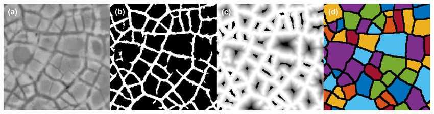
238                                         C. J. Abolt et al.: Ice wedge polygons in high-resolution digital elevation models

30 m resolution (Lara et al., 2018). This dataset offers a static   will permit precise monitoring of surface deformation in
estimate of variation in polygonal form over unprecedented          landscapes covered by repeat airborne surveys.
spatial scales; however, geomorphology was inferred from
the characteristics of pixels larger than typical polygons, pre-
venting inspection of individual features.                          2     Study areas and data acquisition
   Higher resolution approaches to segment imagery into dis-
crete ice wedge polygons have often been motivated by ef-           To demonstrate the flexibility of our approach, we applied it
forts to analyze trough network geometry. On both Earth             simultaneously at two clusters of study sites near Utqiaġvik
and Mars, for example, paleoenvironmental conditions in             and Prudhoe Bay, Alaska, settings with highly divergent ice
remnant polygonal landscapes have been inferred by com-             wedge polygon geomorphology, ∼ 300 km distant from one
paring parameters such as boundary spacing and orienta-             another (Fig. S1 in the Supplement).
tion with systems in modern periglacial terrain (e.g., Pina et
                                                                    2.1    Utqiaġvik
al., 2008; Levy et al., 2010; Ulrich et al., 2011). An early
semi-automated approach to delineating Martian polygons             The first cluster of study sites (Figs. S2–S3) is located within
from satellite imagery was developed by Pina et al. (2006),         10 km of the Beaufort Sea coast in the Barrow Environmen-
who employed morphological image processing operations              tal Observatory, operated by the National Environmental Ob-
to emphasize polygonal boundaries, then applied a watershed         servatory Network (NEON). Mean elevation is less than 5 m
transformation (discussed in Sect. 4.1.3) to identify discrete      above sea level, and vegetation consists of uniformly low-
polygons. This workflow was later applied to lidar-derived          growing grasses and sedges. Mesoscale topography is mostly
DEMs from a landscape outside Utqiaġvik, Alaska, by Wain-          flat but marked by depressions up to 2 m deep associated with
wright et al. (2015), but in their experience and our own, ro-      draws and drained lake beds. In the land cover map of Lara
bust results at spatial scales approaching a square kilometer       et al. (2018), the area is characterized by extensive coverage
or greater were elusive.                                            by both LCPs and HCPs, with occasional lakes and patches
   Our application of CNNs to the task of identifying polyg-        of non-polygonal meadow. Microtopography at the sites re-
onal troughs was inspired by the remarkable solutions that          flects nearly ubiquitous ice wedge development, which be-
CNNs recently have permitted to previously intractable im-          comes occluded in some of the depressions. Ice wedge poly-
age processing problems. Aided by advances in the perfor-           gons are of complex geometry and highly variable area, rang-
mance of graphics processing units (GPUs) over the last             ing from ∼ 10 to > 2000 m2 . An airborne lidar survey was
decade, CNNs have demonstrated unprecedented skill at               flown in August 2012 as part of the U.S. Department of En-
tasks analogous to ice wedge polygon delineation, such as           ergy’s Next Generation Ecosystems Experiment-Arctic pro-
cell membrane identification in biomedical images (Ciresan          gram (https://ngee-arctic.ornl.gov/, last access: 18 January
et al., 2012) or road extraction from satellite imagery (Kestur     2019). The resulting point cloud was processed into a 25 cm
et al., 2018; Xu et al., 2018). Motivated by this potential,        horizontal resolution DEM with an estimated vertical accu-
an exploratory study was recently conducted by Zhang et             racy of 0.145 m (Wilson et al., 2013). In the present study, to
al. (2018), who demonstrated that a sophisticated neural net-       compare algorithm performance on data of variable spatial
work, the Mask R-CNN of He et al. (2017), is capable of the         resolution, the 25 cm DEM was resampled at 50 and 100 cm
end-to-end extraction of ice wedge polygons from satellite-         resolution. Two sites of 1 km2 , here referred to as Utqiaġvik-
based optical imagery, capturing ∼ 79 % of ice wedge poly-          1 and Utqiaġvik-2, were extracted from the DEMs and pro-
gons across a > 134 km2 field site and classifying each as          cessed using our workflow.
HCP or LCP. The authors concluded that the method has po-
tential for the pan-Arctic mapping of polygonal landscapes.         2.2    Prudhoe Bay
Here we explore an alternative approach, using a less com-
plex CNN paired with a set of post-processing operations,           The second cluster of sites (Figs. S4–S11) is approximately
to extract ice wedge polygons from high-resolution DEMs             300 km east of the first and farther inland, located ∼ 40 km
derived from airborne lidar surveys. An advantage of this           south of Prudhoe Bay, Alaska (Fig. S1). As at Utqiaġvik,
method is that training the CNN is rapid (∼ 5 min or less on        vegetation consists almost exclusively of low- and even-
a personal laptop), permitting an iterative workflow in which       growing grasses and sedges. Mesoscale topography is gen-
supplementary data can easily be incorporated to boost skill        erally flat, with a slight (< 4 %) dip toward the northwest. In
in targeted areas. We demonstrate the suitability of this ap-       the land cover map of Lara et al. (2018), the area is primar-
proach to extract ice wedge polygons with very high accu-           ily characterized by HCPs, with smaller clusters of LCPs,
racy (up to 96 % at the kilometer scale), applying it to 10 field   patches of non-polygonal meadow, and occasional lakes. Ice
sites of 1 km2 outside Utqiaġvik and Prudhoe Bay, Alaska.          wedge polygons are generally of more consistent area than
Because our method operates on high-resolution elevation            those of Utqiaġvik, ∼ 400–800 m2 . Airborne lidar data were
data, it enables direct measurement of polygonal microto-           acquired in August 2012 by the Bureau of Economic Geol-
pography, and we anticipate that in the future, the method          ogy at the University of Texas at Austin (Paine et al., 2015)

The Cryosphere, 13, 237–245, 2019                                                        www.the-cryosphere.net/13/237/2019/
C. J. Abolt et al.: Ice wedge polygons in high-resolution digital elevation models 239
Figure 1. Schematic of our iterative workflow for polygon delineation.
and subsequently processed into 25, 50, and 100 cm resolu- wedge polygon. Polygon-scale microtopography was then
tion DEMs. Vertical accuracy was estimated at 0.10 m. As estimated by subtracting the regional topography from the
the Prudhoe Bay survey area is substantially larger than the DEM (Fig. S12). In preparation for passing the data to the
survey area at Utqiaġvik, eight sites of 1 km2 , here referred CNN, microtopography was subsequently converted to 8-
to as Prudhoe-1 through Prudhoe-8, were extracted from the bit grayscale imagery. The minimum intensity (0) was as-
DEMs and processed using our workflow. signed to depressions of 0.7 m or greater, and the maximum
intensity (255) was assigned to ridges of 0.7 m or greater.
These bounds captured > 99 % of pixel values at each study
3 Methods site. Finally, one thumbnail-sized image was created for each
pixel in the microtopography raster, capturing the immedi-
3.1 Polygon delineation algorithm ate neighborhood surrounding it. These thumbnail images
were the direct input to the CNN. The CNN required the
A chart summarizing our iterative workflow is presented in width in pixels of each thumbnail to be an odd multiple of 9;
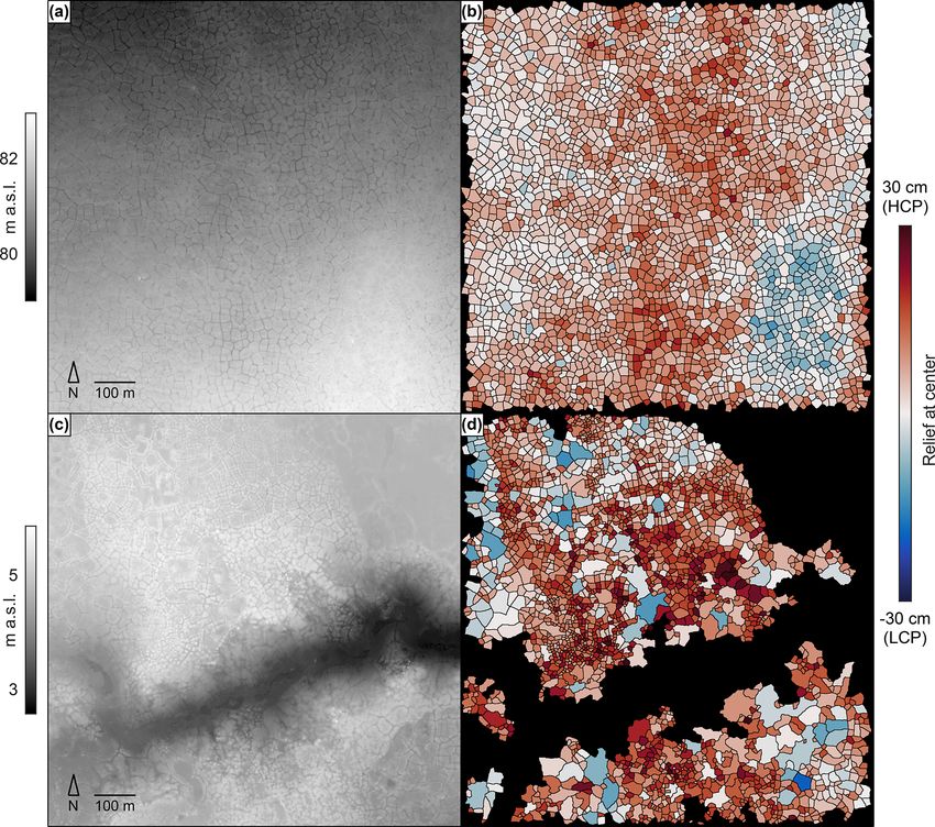
Fig. 1, and several intermediate stages in the polygon delin- therefore, at 50 cm resolution the thumbnails were assigned
eation algorithm are illustrated in Fig. 2. In the first (prepro- a width of 27 pixels (13.5 m), at 25 cm resolution a width
cessing) stage, regional trends were removed from a DEM of 45 pixels (11.25 m), and at 100 cm resolution a width of
(Fig. S12), generating an image of polygonal microtopogra- 27 pixels (27 m). The width of these thumbnails was chosen
phy (Fig. 2a). Next, the microtopographic information was such that each image would contain sufficient spatial context
processed by a CNN, which was trained to use the 27 × 27 for a human observer to distinguish easily between polyg-
neighborhood surrounding each pixel to assign a label of onal boundaries, which typically were demarcated by inter-
“boundary” or “non-boundary” (Fig. 2b). A distance trans- polygonal troughs, and other microtopographic depressions
formation was then applied (i.e., each non-boundary pixel such as LCP centers.
was assigned a negative intensity proportional to its Eu-
clidean distance from the closest boundary), generating a 3.1.2 Convolutional neural network
grayscale image analogous to a DEM of isolated basins, in
which the polygonal boundaries appear as ridges (Fig. 2c). The function of the CNN in our workflow was to identify
Subsequently, a watershed transform was applied to segment pixels likely to represent boundaries. Conceptually, a CNN
the image into discrete ice wedge polygons (Fig. 2d). These is a classification tool that accepts images of a fixed size (in
steps, and a post-processing algorithm used to remove non- our case, the thumbnails described in the previous section)
polygonal terrain from the final image, are described in de- as input and generates categorical labels as output. The CNN
tail below. determines decision criteria through training with a set of
manually labeled images. The architecture of a CNN consists
3.1.1 Preprocessing of a user-defined sequence of components, or layers, which
take inspiration from the neural connections of the visual cor-
In the preprocessing stage, regional topographic trends were tex. We developed our CNN in MATLAB (R2017b) using the
estimated by processing the DEM with a 2-D filter, which Image Processing, Parallel Computing, and Neural Network
assigned to each pixel the mean elevation within a 20 m ra- toolboxes. We purposefully constructed the CNN with an ar-
dius. This radius was chosen such that the area over which chitecture of minimal complexity, to maximize the efficiency
elevation was averaged would be larger than a typical ice of training and application. Here we briefly describe the func-
www.the-cryosphere.net/13/237/2019/ The Cryosphere, 13, 237–245, 2019240 C. J. Abolt et al.: Ice wedge polygons in high-resolution digital elevation models
Figure 2. Illustration of several intermediate stages in our workflow. The CNN processes information stored in 8-bit grayscale imagery
representing microtopography (a), estimated by removing regional trends from the lidar DEM (Fig. S2). The CNN identifies pixels likely
to represent troughs (b). Each non-trough pixel is assigned a negative intensity equal to its distance from a trough (c) and a watershed
transformation is applied to segment the image into discrete polygons (d) (colors randomly applied to emphasize polygonal boundaries).
tion of each layer in our CNN; for more detailed description, a set of non-boundary images for the training deck. Finally,
the reader is directed to Ciresan et al. (2012). for more targeted training that did not require full delineation
Summarized in Table S1, the most important components of a 100 m × 100 m tile, individual instances of boundary or
of our CNN were a single convolutional layer, a max-pooling non-boundary features could also be added to supplement the
layer, and two fully connected layers. In the convolutional training deck, based again on manual delineation (Fig. S13b).
layer, a set of 2-D filters was applied to the input image, Just prior to training, 25 % of the training deck assembled by
generating intermediate images in which features including these methods was set aside to be used for validation.
concavities, convexities, or linear edges were detected. The Once trained, the CNN was executed to assign a label
max-pooling layer downsized the height and width of these of boundary or non-boundary to the thumbnail image cor-
intermediate images by a factor of 3, by selecting the high- responding to each pixel of a study site. These labels were
est intensity pixel in a moving 3 × 3 window with a stride of then reassembled into a binary image of polygon boundaries
3 pixels. Each pixel in the downsized intermediate images (Fig. 2b), which was further processed to extract discrete ice
was then passed as an input signal to the fully connected wedge polygons.
layers, which functioned identically to standard neural net-
works. Two additional components of our CNN were Recti- 3.1.3 Polygon extraction
fied Linear Unit (ReLU) layers, which enhance nonlinearity
by reassigning a value of zero to any negative signals out- After applying the CNN to classify all pixels at a site as
put by a preceding layer, and a softmax layer, which con- boundary or non-boundary, we extracted discrete ice wedge
verted the output from the final fully connected layer into a polygons by applying several standard image processing op-
probability for each categorical label (i.e., boundary or non- erations. The first step was elimination of “salt and pepper”
boundary). noise in the binary image, which we accomplished by elimi-
During training, the weights of the 2-D filters in the convo- nating all contiguous sets of boundary-identified pixels with
lutional layer and the activation functions of the neurons in an area < 20 m2 . This threshold was selected based on the
the fully connected layers were optimized to correctly pre- reasoning that most true boundary pixels should be part of a
dict the labels in a training deck of images. Our workflow continuous network, covering an area arbitrarily larger than
was designed to generate the training deck primarily by pro- 20 m2 , while most false detections should occur in smaller
cessing 100 m × 100 m tiles of manually labeled imagery. In clusters. Next, we applied a distance transform, assigning to
each of these tiles, boundary pixels were delineated by hand every non-boundary pixel a negative intensity equal to its
in a standard raster graphics editor, a process that required Euclidean distance from the nearest boundary. This created
∼ 1 h per tile at 50 cm resolution (Fig. S13a). Our algorithm an intermediate image in which each ice wedge polygon ap-
imported these tiles, identified the geographic coordinates of peared as a valley, surrounded on all or most sides by ridges
each pixel identified as a boundary, then created a thumb- representing the ice wedge network (Fig. 2c). At this stage, to
nail image centered on that pixel from the 8-bit microtopo- prevent over-segmentation, valleys with maximum depths of
graphic imagery. This procedure generated several thousand 1.5 m or less were then identified and merged with the clos-
thumbnail images centered on boundaries from each manu- est neighbor through morphological reconstruction (Soille,
ally delineated tile. Subsequently, an equal number of pix- 2004). The effect of this procedure was to ensure that the
els not labeled as boundaries were selected at random, and algorithm would only delineate polygons whose centers con-
the thumbnail extraction procedure was repeated, generating tained at least one point greater than 1.5 m from the bound-
aries, as field observations indicate that ice wedge poly-
The Cryosphere, 13, 237–245, 2019 www.the-cryosphere.net/13/237/2019/C. J. Abolt et al.: Ice wedge polygons in high-resolution digital elevation models 241
gons tend to measure at least several meters across (Leffing- formance to improve skill (Fig. 1). After four iterations of
well, 1915; Lachenbruch, 1962). Next, watershed segmenta- this approach, the CNN incorporated training data from three
tion was applied to divide the valleys into discrete polygons fully delineated tiles at Utqiaġvik-1 and one at Prudhoe-1,
(Fig. 2d). Our use of this operation was inspired by its in- representing 3 % and 1 % of the sites, respectively. From this
corporation in the polygon delineation method developed by point, we opted to “fine-tune” the CNN by supplementing the
Pina et al. (2006). Conceptually, this procedure was analo- training deck directly with instances of problematic features,
gous to identifying the up-gradient region or area of attrac- rather than using information from fully delineated tiles. Sev-
tion surrounding each local minimum. eral examples of boundary and non-boundary features were
included from Utqiaġvik-1 and Prudhoe-1. Next, to test its
3.1.4 Partitioning of non-polygonal ground extensibility, the CNN was applied across the remaining
sites, and retrained once more. In this final iteration, sev-
In the final stage of delineation, we partitioned out regions eral instances of boundary and non-boundary features (but
of a survey area that had been segmented using the tech- no fully delineated tiles) were incorporated into the training
niques described above, but were unlikely to represent true deck from sites Prudhoe-2, Prudhoe-3, and Prudhoe-4. No
ice wedge polygons. For example, polygons were eliminated training data at all were incorporated from sites Prudhoe-5
from the draw in the southern half of Utqiaġvik-1 (Fig. S2a), through Prudhoe-8 or Utqiaġvik-2. (All training data used
where microtopography was too occluded to permit accu- in the final iteration of our workflow can be viewed in the
rate delineation. Toward this aim, our algorithm individually data and code repository accompanying this article.) Once
analyzed each boundary between two polygons (black line this procedure was complete at 50 cm resolution, training
segments in Fig. 2d), tabulating the number of pixels that decks at 25 and 100 cm resolution were prepared. To gener-
had been identified positively by the CNN (white pixels in ate CNNs comparable to the network trained on 50 cm data,
Fig. 2b). It then dissolved all boundaries in which less than the 25 and 100 cm training decks were constructed using data
half the pixels had been classified positively, merging adja- sampled from identical geographic locations, but manual la-
cent polygons. In practice, this procedure resulted in areas of beling was performed without reference to the labeled 50 cm
non-polygonal terrain being demarcated by unusually large resolution data.
“polygons.” We removed these areas by partitioning out any After the CNN was trained and applied across all study
polygon with an area greater than 10 000 m2 , a threshold se- sites, we quantified the performance of the polygon delin-
lected to be arbitrarily larger than most real ice wedge poly- eation algorithm through manual validation. At each site, we
gons. This procedure had the strengths of being conceptually first calculated the total area and number of polygons ex-
simple and providing a deterministic means of partitioning tracted from the landscape. We then randomly sampled 500
non-polygonal terrain from the rest of a survey area. of the computer-delineated polygons, and classified each as
either whole, fragmentary, conglomerate, or false. Fragmen-
3.2 Microtopographic analysis
tary polygons were defined as computer-delineated polygons
To demonstrate the capabilities of our workflow for microto- that included less than 90 % of one real polygon, conglomer-
pographic analysis, we developed a simple method for mea- ate polygons were defined as computer-delineated polygons
suring the relative elevation at the center of each delineated comprising parts of two or more real polygons, and false
polygon, serving as a proxy for LCP or HCP form. In each polygons were defined as computer-delineated polygons oc-
polygon, we first applied a distance transform, calculating cupying terrain in which no polygonal pattern was deemed
the distance from the closest boundary of all interior pixels. visible to the human evaluator. The percentage of computer-
We then divided the area of the polygon in half at the me- delineated polygonal terrain corresponding to each class was
dian distance from boundaries, designating a ring of “outer” then calculated by number of polygons and by area. This pro-
pixels and an equally sized core of center pixels. Microtopo- cedure was completed for all 10 study sites at 50 cm data res-
graphic relief was then estimated as the difference in mean olution, and for sites Prudhoe-1 and Utqiaġvik-1 at 25 and
elevation between the center and outer pixels. 100 cm resolution.
3.3 Case study experimental design
4 Results and discussion
The case study was first conducted using topographic data
at 50 cm resolution, then repeated at 25 and 100 cm res- 4.1 Training speed and accuracy
olution. Training was focused primarily on sites Prudhoe-
1 and Utqiaġvik-1. Leveraging the rapid training and ap- Due to the compact architecture of our CNN, training speeds
plication times of our CNN, we manually delineated one at 50 cm resolution and 100 cm resolution were rapid. At
100 m × 100 m tile of imagery at a time from either site, 50 cm resolution, the training procedure operated on a deck
trained the CNN, extracted results from both sites, then in- of ∼ 36 000 thumbnail images. Executed on a personal lap-
troduced additional training data from regions of poor per- top with an Intel i7 CPU and a single GeForce MX150
www.the-cryosphere.net/13/237/2019/ The Cryosphere, 13, 237–245, 2019242 C. J. Abolt et al.: Ice wedge polygons in high-resolution digital elevation models
Table 1. Results of manual validation at 50 cm data resolution (sites are 1 km2 ).
% of polygons % of polygons
by instance by area
Polygons identified
Polygonal area (%)
Non-polygonal
Non-polygonal
Conglomerate
Conglomerate
Fractional
Fractional
Whole
Whole
Site
Utqiaġvik-1 2555 68.3 94.2 2.2 2.2 1.4 86.9 1.4 7.5 4.2
Utqiaġvik-2 2613 68.8 91.6 2.8 5.6 0.0 79.9 3.6 16.5 0.0
Prudhoe-1 3227 99.9 95.6 2.8 1.4 0.2 96.3 2.2 1.4 0.0
Prudhoe-2 4685 94.5 91.6 1.4 7.0 0.0 87.7 1.7 10.6 0.0
Prudhoe-3 1112 48.2 91.2 3.6 5.2 0.0 82.3 4.2 13.4 0.0
Prudhoe-4 1956 60.4 88.2 4.2 7.2 0.4 81.4 3.2 14.9 0.5
Prudhoe-5 2969 77.9 91.8 4.0 4.2 0 87.7 1.7 10.6 0
Prudhoe-6 1605 65.5 85.8 5.4 8.2 0.4 69.5 4.8 22.1 3.4
Prudhoe-7 1348 47.3 94.0 2.2 3.6 0.2 90.5 1.7 7.9 0.0
Prudhoe-8 3288 100 96.0 2.2 1.6 0.2 95.2 1.5 3.2 0.0
GPU, accuracies > 97 % on the training deck and > 95 % nal geometry, such as Prudhoe-1, Prudhoe-7, and Prudhoe-8
on the validation deck of thumbnails were achieved in less (Figs. S4, S10, S11). In contrast, performance was weakest at
than 5 min. At 100 cm resolution, the procedure operated on sites such as Utqiaġvik-2 or Prudhoe-6 (Figs. S2, S9), where
∼ 12 000 thumbnail images, achieving comparable levels of considerable swaths of terrain are characterized by faint mi-
accuracy within 90 s. These speeds enable the iterative ap- crotopography, as ice wedge polygons appear to grade into
proach to training on which our workflow is based (Fig. 1), non-polygonal terrain. In such locations, polygonal bound-
as the CNN can be retrained quickly to incorporate new data aries frequently went undetected, resulting in the delineation
when applied across increasingly large areas. of unrealistically large conglomerate polygons. In general,
Using 25 cm resolution data, the training procedure op- the results of the delineation clearly illustrate that the polyg-
erated on a set of ∼ 115 000 thumbnail images. Accuracies onal network at Utqiaġvik possesses more complex geometry
> 97 % on the training deck and > 95 % on the validation than Prudhoe Bay, with many instances in which secondary
deck were once more obtained, but training required just un- or tertiary ice wedges appear to subdivide larger ice wedge
der 1 h on the same computer. This substantial increase to polygons.
training time is attributable to the facts that more thumbnail Although simple, our post-processing procedure for par-
images were processed, and the number of pixels in each titioning out non-polygonal ground from the results was
thumbnail was larger, making execution of the CNN more generally accurate. Examples of features successfully re-
computationally expensive. moved from the 50 cm resolution DEMs included thaw
lakes (Figs. S6–S10), drained thaw lake basins (Fig. S2),
4.2 Delineation speed and validation streambeds (Figs. S5, S9), non-polygonal marsh (Figs. S3,
S7, S9), shallow ponds (Fig. S7), and the floodplain of a
braided stream (Fig. S10). Because the partitioning proce-
Operating at 50 cm resolution, delineation of ice wedge poly-
dure removed areas with a low density of boundaries iden-
gons within a 1 km2 field site required ∼ 2 min, including
tified by the CNN, we found that it could be trained effi-
application of the CNN and subsequent post-processing. Re-
ciently by supplementing the training deck with extra ex-
sults generally were very accurate; across study sites, ∼
amples of non-boundary thumbnails extracted from these re-
1000–5000 ice wedge polygons were detected per square
gions. Across the study sites, we encountered almost no cases
kilometer, of which 85–96 % were estimated as “whole” dur-
in which well-defined polygons were mistakenly partitioned
ing manual validation, representing 70–96 % of the polygo-
out. Instances of non-polygonal ground mistakenly classi-
nal ground by area (Table 1). The most common type of error
fied as polygonal accounted for less than 1 % of machine-
at all sites with < 95 % accuracy was incorrect aggregation
delineated polygons by area.
of several real ice wedge polygons into a single feature. Un-
When the delineation algorithm was repeated using data at
surprisingly, performance was strongest at sites with clearly
100 cm resolution, delineation speeds increased somewhat,
defined polygon boundaries and relatively simple polygo-
The Cryosphere, 13, 237–245, 2019 www.the-cryosphere.net/13/237/2019/C. J. Abolt et al.: Ice wedge polygons in high-resolution digital elevation models 243
Figure 3. DEMs and estimates of polygonal relief at sites Prudhoe-1 (a, b) and Utqiaġvik-1 (c, d). Polygons crossing the boundaries of study
sites are removed in (b, d).
but performance dropped significantly, with greater declines 50 cm resolution; however, performance speeds were gen-
occurring in the challenging environment of Utqiaġvik (Ta- erally inhibitory to our workflow, as delineation required
ble S2). We attribute declines in performance to an obscura- ∼ 50 min km−2 . We therefore conclude that 50 cm resolution
tion of fainter polygonal boundaries at this resolution, and data are optimal for our analysis.
to decreases in the amount of contextual information that
can be derived from the neighborhood of any given pixel, 4.3 Measurement of polygonal microtopography
reducing the capacity for the algorithm to distinguish be-
tween polygonal troughs and other microtopographic depres- The time required to execute our procedure for measuring
sions (Fig. S14). Somewhat surprisingly, performance also polygonal microtopography varied from ∼ 10–30 s km−2 at
declined slightly using data at 25 cm resolution, with larger 50 cm resolution, depending on the number of polygons de-
fractions of fragmentary and false polygons accounting for lineated. A comparison of calculated relief at polygon cen-
most of the increases in errors (Table S2). We attribute these ters between Prudhoe-1 and Utqiaġvik-1 reveals that both
mistakes to the larger number of distinguishable features in sites are characterized by the prevalence of HCPs, which
the higher resolution data, leading the algorithm to more surround smaller clusters of LCPs (Fig. 3). Relief tends to
frequently mistake features not encountered in the training be more extreme at Utqiaġvik, with the relative elevation of
dataset as boundary pixels. As the imagery nonetheless is of polygon centers commonly approaching 20–30 cm. Our au-
sufficient resolution for our purposes, we anticipate that, with tomated calculations of relief align well with visual inspec-
augmentations to the training dataset, performance at 25 cm tion of the DEMs, as rimmed LCPs are consistently assigned
resolution could improve and even exceed performance at negative center elevations. To the best of our knowledge, our
results represent the first direct measurement of polygonal re-
www.the-cryosphere.net/13/237/2019/ The Cryosphere, 13, 237–245, 2019244 C. J. Abolt et al.: Ice wedge polygons in high-resolution digital elevation models
lief at the kilometer scale, demonstrating a spectrum of cen- tion of the watershed transformation. We acknowledge that,
ter elevations rather than a binary classification into LCP or because the surface expression of ice wedges is sometimes
HCP. We anticipate these measurements may be useful for subtle or nonexistent, ground-based delineation methods are
further investigations into relationships between microtopog- the highest accuracy approach to mapping ice wedge net-
raphy, soil moisture, and carbon fluxes (e.g., Wainwright et works (Lousada et al., 2018). Nonetheless, by segmenting
al., 2015). machine-delineated networks into individual boundaries, our
workflow permits the estimation of network statistics at spa-
4.4 Comparison with Mask R-CNN and future tial scales unattainable through on-site surveying.
applications
Several key differences are apparent between the workflow 5 Conclusions
presented in this paper (hereafter termed the CNN-watershed
approach) and a recent implementation of Mask R-CNN for A relatively simple CNN paired with a set of common im-
the mapping of ice wedge polygons (Zhang et al., 2018), re- age processing techniques is capable of extracting polygons
vealing relative strengths of each approach. An advantage of of highly variable size and geometry from high-resolution
the CNN-watershed approach, stemming from its sparse neu- DEMs of diverse tundra landscapes. Successful application
ral architecture, is that training times are extremely rapid, fa- of the CNN is facilitated by its sparse neural architecture,
cilitating iterative improvements to skill (Fig. 1). In contrast, which permits rapid training, testing, and incorporation of
although inference times using the CNN-watershed approach new data to improve skill. The optimal spatial resolution
are reasonable, extraction of ice wedge polygons over broad for DEMs processed using the workflow is ∼ 50 cm. Poten-
landscapes is several times faster using Mask R-CNN, with tial applications for the technology include the generation of
a reported time of ∼ 21 min for inference over 134 km2 of high-resolution maps of land cover by polygon type, the pre-
terrain (Zhang et al., 2018). Because the CNN-watershed ap- cise quantification of microtopographic deformation in areas
proach operates on high-resolution DEMs, it enables direct covered by repeat airborne surveys, and the rapid extraction
quantification of polygonal relief, whereas Mask R-CNN in- of center elevations and boundary parameters including spac-
stead produces a binary classification of each polygon as ei- ing and orientation. These capabilities can improve under-
ther LCP or HCP. The CNN-watershed approach is therefore standing of environmental influences on network geometry
useful for generating unique datasets summarizing polygonal and facilitate assessments of contemporary landscape evolu-
geomorphology, demonstrating high performance at spatial tion in the Arctic.
scales typical of airborne surveys using lidar or photogram-
metry to produce high-resolution DEMs. In comparison, be-
Data availability. Data and code are available at
cause Mask R-CNN has been trained to operate on satellite-
https://doi.org/10.5821/zenodo.2537167 (Abolt et al., 2018).
derived optical imagery with global coverage, it is uniquely
well suited for application across very broad regions, with the
potential to generate pan-Arctic maps of land cover by poly- Author contributions. CJA and MHY conceived the project. CJA
gon type. Because of differences in training and inference developed the algorithm with guidance from MHY and ALA. CJW
procedures and the spatial scales at which they ideally oper- developed the lidar DEM for Utqiagvik, and all authors contributed
ate, the training data requirements and accuracy of the two to the two-site experimental design. CJA wrote the paper with as-
approaches are difficult to compare directly; nonetheless, in sistance from all authors.
several aspects, performance appears to be similar (Sect. S1).
Because the CNN-watershed approach generates direct
measurements of polygonal microtopography, one applica- Competing interests. The authors declare that they have no conflict
tion to which it is uniquely amenable is the precise monitor- of interest.
ing of microtopopographic deformation in areas covered by
repeat airborne surveys. Through such analysis, we anticipate
that it will permit the polygon-level quantification of ground Acknowledgements. We are grateful for the support provided for
subsidence over time spans of years, potentially yielding new this research, which included the Next Generation Ecosystem
insights into the vulnerability of various landscape units to Experiments Arctic (NGEE-Arctic) project (DOE ERKP757),
funded by the Office of Biological and Environmental Research
thermokarst. An additional research problem to which the
in the U.S. Department of Energy Office of Science, and the
CNN-watershed approach is well suited is the quantification
NASA Earth and Space Science Fellowship program, for an award
of polygonal network parameters, such as boundary spac- to Charles J. Abolt (80NSSC17K0376). We thank Ingmar Nitze
ing and orientation, to explore relationships to environmental (Alfred Wegener Institute for Polar and Marine Research) and
factors such as climate (e.g., Pina et al., 2008; Ulrich et al., Weixing Zhang (University of Connecticut) for highly constructive
2011). These boundaries (black line segments in Figs. 2d, feedback during peer review, and Dylan Harp (Los Alamos
3b and d) are naturally delineated through the implementa- National Laboratory) for helpful conversations during manuscript
The Cryosphere, 13, 237–245, 2019 www.the-cryosphere.net/13/237/2019/C. J. Abolt et al.: Ice wedge polygons in high-resolution digital elevation models 245
preparation. We acknowledge the Texas Advanced Computing E., Schulla, J., Tape, K. D., Walker, D. A., Wilson, C. J., Yabuki,
Center (TACC) at the University of Texas at Austin for providing H., and Zona, D.: Pan-Arctic ice-wedge degradation in warming
HPC resources that have contributed to the results reported within permafrost and its influence on tundra hydrology, Nat. Geosci.,
this paper. 9, 312–318, https://doi.org/10.1038/ngeo2674, 2016.
Lousada, M., Pina, M., Vieira, G., Bandeira, L., and Mora, C.: Eval-
Edited by: Moritz Langer uation of the use of very high resolution aerial imagery for accu-
Reviewed by: Ingmar Nitze and Weixing Zhang rate ice-wedge polygon mapping (Adventdalen, Svalbard), Sci.
Total Environ., 615, 1574–1583, 2018.
Paine, J. G., Andrews, J. R., Saylam, K., and Tremblay, T. A.: Air-
borne LiDAR-based wetland and permafrost-feature mapping on
References an Arctic Coastal Plain, North Slope, Alaska, in: Remote Sens-
ing of Wetlands: Applications and Advances, edited by: Tiner,
Abolt, C. J., Young, M. H., Atchley, A. L., and Brown, R. W., Klemas, V. V., and Lang, M. W., CRC Press, Boca Raton,
C. J.: CNN-watershed: A machine-learning based tool for FL, USA, 413–434, 2015.
delineation and measurement of ice wedge polygons in Pina, P., Saraiva, J., Bandeira, L., and Barata, T.: Identification of
high-resolution digital elevation models, Zenodo repository, Martian polygonal patterns using the dynamics of watershed con-
https://doi.org/10.5821/zenodo.2537167, 2018. tours, in: Image Analysis on Recognition, edited by: Campilho,
Ciresan, D., Giusti, A., Gambardella, L. M. and Schmidhuber, J.: A. and Kamel, M., Springer-Verlag, Berlin-Heidelberg, 691–699,
Deep neural networks segment neuronal membranes in electron 2006.
microscopy images, in: Advances in Neural Information Process- Pina, P., Saraiva, J., Bandeira, L., and Antunes, J.: Polygonal ter-
ing Systems 25, edited by: Pereira, F., Burges, C. J. C., Bot- rains on Mars: A contribution to their geometric and topological
tou, L., and Weinberger, Q., Curran Associates, Inc., 2843–2851, characterization, Planet. Space Sci., 56, 1919–1924, 2008.
2012. Raynolds, M. K., Walker, D. A., Ambrosius, K. J., Brown,
He, K., Gkioxari, G., Dollar, P., and Girshick, R.: Mask R-CNN, J., Everett, K. R., Kanevskiy, M., Kofinas, G. P., Ro-
in: Proceedings of the 2017 IEEE International Conference on manovsky, V. E., Shur, Y., and Webber, P. J.: Cumula-
Computer Vision, IEEE, Piscataway, NJ, USA, 2017. tive geoecological effects of 62 years of infrastructure and
Jorgenson, M. T., Shur, Y. L., and Pullman, E. R.: Abrupt increase climate change in ice-rich permafrost landscapes, Prudhoe
in permafrost degradation in Arctic Alaska, Geophys. Res. Lett., Bay Oilfield, Alaska, Global Change Biol., 20, 1211–1224,
33, L02503, https://doi.org/10.1029/2005GL024960, 2006. https://doi.org/10.1111/gcb.12500, 2014.
Jorgenson, M. T., Kanevskiy, M., Shur, Y., Moskalenko, N., Brown, Soille, P.: Morphological Image Analysis, Springer-Verlag: Berlin
D. R. N., Wickland, K., Striegl, R. and Koch, J.: Role of ground Heidelberg, 2004.
ice dynamics and ecological feedbacks in recent ice wedge Ulrich, M., Hauber, E., Herrzschuh, U., Hartel, S., and Schirrmeis-
degradation and stabilization, J. Geophys. Res.-Earth Surf., 120, ter, L.: Polygon pattern geomorphometry on Svalbard (Norway)
2280–2297, https://doi.org/10.1002/2015JF003602, 2015. and western Utopia Planitia (Mars) using high resolution stereo
Kestur, R., Farooq, S., Abdal, R., Mehraj, E., Narasipura, O. and remote-sensing data, Geomorphology, 134, 197–216, 2011.
Mudigere, M.: UFCN: A fully convolutional neural network for Wainwright, H. M., Dafflon, B., Smith, L. J., Hahn, M. S., Curtis, J.
road extraction in RGB imagery acquired by remote sensing from B., Wu, Y., Ulrich, C., Peterson, J. E., Torn, M. S., and Hubbard,
an unmanned aerial vehicle, J. Appl. Remote Sens., 12, 016020, S. S.: Identifying multiscale zonation and assessing the relative
https://doi.org/10.1117/1.JRS.12.016020, 2018. importance of polygon geomorphology on carbon fluxes in an
Lachenbruch, A. H.: Mechanics of thermal contraction cracks and Arctic tundra ecosystem, J. Geophys. Res.-Biogeosci., 120, 788–
ice-wedge polygons in permafrost, Special Paper, Geological So- 808, https://doi.org/10.1002/2014JG002799, 2015.
ciety of America, New York, 1962. Wilson, C., Gangodagamage, C., and Rowland, J.: Digital eleva-
Lara, M. J., McGuire, A. D., Euskirchen, E. S., Tweedie, C. E., tion model, 0.5 m, Barrow Environmental Observatory, Alaska,
Hinkel, K. M., and Skurikhin, A. N.: Polygonal tundra geomor- 2012, Next Generation Ecosystem Experiments Arctic Data Col-
phological change in response to warming alters future CO2 and lection, Oak Ridge National Laboratory, US Department of En-
CH4 flux on the Barrow Peninsula, Global Change Biol., 21, ergy, https://doi.org/10.5440/1109234, 2013.
1634–1651, 2015. Xu, Y. Y., Xie, Z., Feng, Y. X., and Chen, Z. L.: Road
Lara, M. J., Nitze, I., Grosse, G., and McGuire, A. D.: extraction from high-resolution remote sensing im-
Tundra landform and vegetation trend maps for the Arc- agery using deep learning, Remote Sens., 10, 1461,
tic Coastal Plain of northern Alaska, Sci. Data, 5, 180058, https://doi.org/10.3390/rs10091461, 2018.
https://doi.org/10.1038/sdata.2018.58, 2018. Zhang, W., Witharana, C., Liljedahl, A., and Kanevskiy, M.:
Leffingwell, E. K.: Ground-ice wedges: The dominant form of Deep convolutional neural networks for automated charac-
ground-ice on the north coast of Alaska, J. Geol., 23, 635–654, terization of Arctic ice-wedge polygons in very high spa-
1915. tial resolution aerial imagery, Remote Sens., 10, 1487,
Levy, J. S., Marchant, D. R., and Head, J. W.: Thermal contraction https://doi.org/10.3390/rs10091487, 2018.
crack polygons on Mars: A synthesis from HiRISE, Phoenix, and
terrestrial analogue studies, Icarus, 226, 229–252, 2010.
Liljedahl, A. K., Boike, J., Daanen, R. P., Fedorov, A. N., Frost,
G. V., Grosse, G., Hinzman, L. D., Iijma, Y., Jorgenson, J. C.,
Matveyeva, N., Necsoiu, M., Raynolds, M. K., Romanovsky, V.
www.the-cryosphere.net/13/237/2019/ The Cryosphere, 13, 237–245, 2019You can also read