BUG PREDICTION WITH MACHINE LEARNING - BLOODHOUND 0.1 GUSTAV REHNHOLM FELIX RYSJÖ - DIVA PORTAL

Bug Prediction
with Machine Learning
Bloodhound 0.1

Gustav Rehnholm
Felix Rysjö

Faculty of Health, Science and Technology
Computer Science
Bachelor thesis 15hp
Supervisor: Sebastian Herold
Examiner: Mohammad Rajiullah
Date: 2021­05­31

Foreword

We want to thank Lukas Schulte, who helped us with great patience to get his program
cdbs to work with our program Bloodhound. Also, a big thank to Sebastian Herold, our
supervisor, who helped us stay on track during this thesis.

                                            i

ii   FOREWORD

Abstract

Introduction Bugs in software is a problem that grows over time if they are not dealt
with in an early stage, therefore it is desirable to find bugs as early as possible. Bugs
usually correlate with low software quality, which can be measured with different code
metrics. The goal of this thesis is to find out if machine learning can be used to predict
bugs, using code metric trends.

Method To achieve the thesis goal a program was developed, which will be called
Bloodhound, that analyses code metric trends to predict bugs using the machine learning
algorithm k nearest neighbour. The code metrics required to do so is extracted using the
program cdbs, which in turn uses the program SonarQube to create the source code
metrics.

Results Bloodhound were trained with a time-frame of 42 days between the dates
June 1, 2016 to July 13, 2016 containing 202 commits and 312 changed files from the
JabRef repository. The files were changed on average 1.5 times. Bloodhound never
found more than 25% of the bugs and of its bug predictions, was right at most 42% of
the time.

Conclusion Bloodhound did not succeed in predicting bugs. But that was most likely
because the time frame was too short to generate any significant trends.

Keywords Bug prediction, Machine learning, Time series classification

                                           iii

iv   ABSTRACT

Contents

Foreword                                                                                   i

Abstract                                                                                 iii

Figures                                                                                  vii

Tables                                                                                   ix

1 Introduction                                                                            1
   1.1     Background . . . . . . . . . . . . . . . . . . . . . . . . . . . . . . . .     1
   1.2     Problem Description . . . . . . . . . . . . . . . . . . . . . . . . . . .      1
   1.3     Goal and Purpose . . . . . . . . . . . . . . . . . . . . . . . . . . . . .     2
   1.4     Summary of Result . . . . . . . . . . . . . . . . . . . . . . . . . . . .      2
   1.5     Ethical and Societal Issues . . . . . . . . . . . . . . . . . . . . . . . .    3
   1.6     Distribution of Work . . . . . . . . . . . . . . . . . . . . . . . . . . .     3
   1.7     Scope of Thesis . . . . . . . . . . . . . . . . . . . . . . . . . . . . . .    4
   1.8     Disposition . . . . . . . . . . . . . . . . . . . . . . . . . . . . . . . .    4

2 Background                                                                              7
   2.1     Metrics . . . . . . . . . . . . . . . . . . . . . . . . . . . . . . . . . .    7
   2.2     Machine Learning Algorithms . . . . . . . . . . . . . . . . . . . . . .        8
   2.3     Related Work . . . . . . . . . . . . . . . . . . . . . . . . . . . . . . .    10

                                             v

vi                                                                            CONTENTS

     2.4   Summary . . . . . . . . . . . . . . . . . . . . . . . . . . . . . . . . .      11

3 Method                                                                                  13
     3.1   Bloodhounds Input . . . . . . . . . . . . . . . . . . . . . . . . . . . .      13
     3.2   Design Overview . . . . . . . . . . . . . . . . . . . . . . . . . . . . .      14
     3.3   Code Trend Metric Extraction . . . . . . . . . . . . . . . . . . . . . .       15
     3.4   Bug Fix Commit Extraction . . . . . . . . . . . . . . . . . . . . . . . .      16
     3.5   Classifier Training and Evaluation . . . . . . . . . . . . . . . . . . . .      18
     3.6   Summary . . . . . . . . . . . . . . . . . . . . . . . . . . . . . . . . .      20

4 Results                                                                                 21
     4.1   Evaluation . . . . . . . . . . . . . . . . . . . . . . . . . . . . . . . . .   21
           4.1.1   Evaluation Setting . . . . . . . . . . . . . . . . . . . . . . . .     21
           4.1.2   Evaluation Results . . . . . . . . . . . . . . . . . . . . . . . .     22
           4.1.3   Discussion of Evaluation Results . . . . . . . . . . . . . . . . .     22
     4.2   Problems and Issues . . . . . . . . . . . . . . . . . . . . . . . . . . . .    23
           4.2.1   Cdbs . . . . . . . . . . . . . . . . . . . . . . . . . . . . . . .     23
           4.2.2   Cloud Computing . . . . . . . . . . . . . . . . . . . . . . . . .      24
     4.3   Summary . . . . . . . . . . . . . . . . . . . . . . . . . . . . . . . . .      25

5 Conclusions                                                                             27

Bibliography                                                                              29

Appendix                                                                                  34

A Results from Bloodhound                                                                 37

List of Figures

 2.1   K-NN example . . . . . . . . . . . . . . . . . . . . . . . . . . . . . .     9

 3.1   Code metric trends . . . . . . . . . . . . . . . . . . . . . . . . . . . .   14
 3.2   Design Bloodhound . . . . . . . . . . . . . . . . . . . . . . . . . . . .    15
 3.3   Preprocessing for the model . . . . . . . . . . . . . . . . . . . . . . .    19

 4.1   Model evaluation . . . . . . . . . . . . . . . . . . . . . . . . . . . . .   22

 A.1 1-NN . . . . . . . . . . . . . . . . . . . . . . . . . . . . . . . . . . .     37
 A.2 3-NN . . . . . . . . . . . . . . . . . . . . . . . . . . . . . . . . . . .     37
 A.3 5-NN . . . . . . . . . . . . . . . . . . . . . . . . . . . . . . . . . . .     37
 A.4 7-NN . . . . . . . . . . . . . . . . . . . . . . . . . . . . . . . . . . .     38
 A.5 11-NN . . . . . . . . . . . . . . . . . . . . . . . . . . . . . . . . . . .    38
 A.6 13-NN . . . . . . . . . . . . . . . . . . . . . . . . . . . . . . . . . . .    38

                                        vii

viii   LIST OF FIGURES

List of Tables

 3.1   Code metrics for Bloodhound . . . . . . . . . . . . . . . . . . . . . . .   17

                                        ix

x   LIST OF TABLES

Chapter 1

Introduction

1.1 Background

Bugs in software are a problem, and it is unavoidable that some bugs will exists for large
programs. The problem with bugs grow the longer they exist in the program.
    The Celerity webpage describes an example based upon information from the Sys-
tems Sciences Institute at IBM [1] that describe the cost of a bug depending on how fast
it can be identified. The example tells that if the cost of a bug is $100 if it is found in the
gathering of requirements phase. If the same bug is instead found during the QA testing
phase, it could cost $1,500. Finally, if the bug is identified during the production phase,
its cost could be $10,000.[2]
    Therefore it is desirable to find and fix existing bugs as early as possible. Or even
better, what if it could be predicted where bugs are likely to happen in the future?

1.2 Problem Description

Bugs do usually have a correlation with bad code quality, which can be measured with
different kinds of code metrics [3]. Bugs correlation with code quality have been proven

                                              1

2                                                    CHAPTER 1. INTRODUCTION

by different researchers by finding that files containing antipatterns, coding practices
with low quality, and/or code smell, signs of low code quality, lead to a higher density
of bugs [4, 5]. Therefore to predict bugs one can look for a correlation between code
metrics and bugs. This thesis will use metrics about the source code to find code quality
trends that are pointing in the wrong direction to predict bugs. More precisely the
metrics cyclomatic complexity, issues such as code smell and vulnerabilities, comment
density, the average length of a function and how many lines of code there are.

1.3 Goal and Purpose

The goal is to create a program, which will be called Bloodhound, that with machine
learning(ML) will predict bugs; for the purpose to explore the possibilities to predict
bugs with time series classification(TSC) of code metric trends. To extract the code
metrics Schulte’s tool cdbs will be used.

1.4 Summary of Result

Bloodhound were trained on a time-frame of 202 commits and performed as best when
the classifier k nearest neighbour (K-NN) had the k value 5. But the bug predictions
were lower than other bug prediction programs with the likely reason that the time-
frame was too short. A longer time-frame would have been gathered if not that the
tool for code metric extraction cdbs stopped working during the development process
of Bloodhound.

1.5. ETHICAL AND SOCIETAL ISSUES                                                      3

1.5 Ethical and Societal Issues

Prediction of bugs could have a significant impact on economics. The larger the com-
pany, the more customers they typically have. If said company is providing a system-
based product that contains one or more hidden bugs. The system could malfunction
and potentially affect every customer and cost the company a lot of money if this
malfunction is significant enough.
   As mentioned earlier the cost of a software bug can be exponentially high when
discovered to late. As an example the webpage [1] provides three famous examples of
bugs that costed companies fortunes. One of these examples are when NASA launched
the Mariner 1 spacecraft that was USA’s first attempt at sending a spacecraft to Venus.
A small code issue caused the guidance signals to be incorrect and caused the spacecraft
to veer of course and so was instructed to self-destruct and costed NASA $18 million at
the time.
   Another ethical viewpoint of the metric analysis is evaluation of people. Among the
possible metrics for this program was metrics that told the reader which member made
a certain commit. By using this information, the tool can create a model that predicts
bugs within files based upon a certain person changing the code. Not only can this be
deeply offensive to a person, but it can also be false since the person could be tasked
with a complex part of the system at that moment. This would lead to the tool predicting
bugs even when the person is working on a simple task.

1.6 Distribution of Work

When it came to how the general work of the project was divided. During the first
month of the project both Rehnholm and Rysjö spent their hours researching the same
things. This was so that well informed decisions could be made of how the project
should be structured. Once the implementation phase had begun, Rysjö and Rehnholm

4                                                    CHAPTER 1. INTRODUCTION

worked together to create the general structure of the code by working on the same
code together with pair programming. Since a big part of the project relied on Lukas
Schulte’s tool cdbs, Rysjö was decided to be responsible for running and handling the
tool as well as keeping up contact with Schulte. Rehnholm had further responsibility
for the ML model and the final implementation changes that was requested by Sebastian
Herold.
    During the course of the project parts of this paper was written when enough infor-
mation was gathered to do so by both Rysjö and Rehnholm. Once the final implementa-
tions were made Rysjö started writing the paper while Rehnholm joined Rysjö as soon
as the last implementation was complete. At that point, both Rysjö and Rehnholm spent
their hours on the paper until completion.

1.7 Scope of Thesis

Because Bloodhounds heavy use of the program cdbs, cdbs limitations on which pro-
grams it can analyse; will also be true for Bloodhound. Which is, that only programs
which are written in Java (but only up to Java 13), that use Gradle, been developed with
the version control system git and are stored in GitHub can be analysed by Bloodhound
[6]. Also, the available metrics for Bloodhound are limited by what cdbs provides.
Because Bloodhounds goal is to determine the possibility to predict bugs; optimizations,
proper testing and a user-friendly interface are outside Bloodhounds scope.

1.8 Disposition

In chapter 2, there is information on the tools and algorithms that has been chosen
for this thesis. Chapter 3 tell about the design and implementation of Bloodhound.
Chapter 4 shows the results that was gathered from Bloodhound and last chapter 5,

1.8. DISPOSITION                                      5

which conclusions can be gathered from this thesis.

6   CHAPTER 1. INTRODUCTION

Chapter 2

Background

This chapter shows the theory behind the core concepts of Bloodhound.

2.1 Metrics

Code metrics are a method to quantify attributes in software, which are used to achieve
a measurable insight to a software’s quality [7].There are 3 types of metrics that can be
used for software quality [8]:

    • Source Code Metrics - That measure a code on the fundamental source code
      level.

    • Development Metrics - These metrics measure the custom software development
      process itself.

    • Testing Metrics - These metrics help the evaluation of how functional a product
      is.

   This thesis will be using software metrics provided by a metric calculation software
created by a third party. Software metrics provide measured data at a specific point

                                           7

8                                                                   CHAPTER 2. BACKGROUND

in time which can be useful. However, by looking at the same type of metric over a
specified time period, trends can be identified. This information can improve an insight
of a program’s development that a single metric cannot. An example of a code metric
trend is to measure the number of code-lines, with the intention that a rapid change will
correlate to bugs.
     The third party software that is responsible for measuring and calculating the source
code metrics that Bloodhound uses is called cdbs. Cdbs is a metric calculation tool
developed my Lukas Schulte that collects commits from a GitHub repository and uses
SonarQube to create source code metrics [9].
     There are multiple metrics one can look at to find code smell. SonarQube has
different kinds of categories for the metrics, such as duplications (lines, files); amount
of different kinds of issues; lines of comments; functions; how tests have been used
and complexity of the code. When choosing metrics, one needs to take bias            1   into
consideration.
     The source code metrics that are primarily being tested within this thesis are com-
plexity, vulnerabilities, code smells, comment_line_density. The source code metric
code_lines will be both tested and used to calculate a multitude of features whom’s
magnitude will be divided by the over all size of the file.

2.2 Machine Learning Algorithms

ML is a computer algorithm that improves automatically through the use of data. ML
algorithms build a model based on training data, in order to make predictions or de-
cisions without being explicitly programmed to do so. One group of ML algorithms
are classifiers, which predicts a class of given data points. A classifier, is of the type
supervised learning, which means that the input will be labelled [10, 11]. There are
    1 To   have multiple metrics that depends on the same thing, like code length

2.2. MACHINE LEARNING ALGORITHMS                                                          9

multiple classifiers but one that are simple to implement and generally performs well is
K-NN [12, 13, 14, 15, 16, 17].

   The K-NN algorithm works by setting an unclassified data point to the same group
as the majority of the k closest data points(where k is a positive integer). For example
figure 2.1 shows that if k is 4, the data point ? will look for its closest 4 data points;
which are one green, one blue and two red. Because there are more red than green and
blue; ? will be predicted as a red data point [16].

                               Figure 2.1: K-NN example

   When a set of data are ordered, as in a time-frame, it is called TSC. Which will be
the case for this thesis classifier, because it will look at changes over time. To implement
K-NN for a TSC problem, one need to either calculate the distance in time with help of
another algorithm, usually dynamic time warping [13] or reinterpreted the time series
as a primitive values, such as a slope.

   When training a classifier, there is a risk that the classifier will be overfitted, which
means that the classifier gets very good at predicting the data it was trained on, but
nothing else. Because of that, the data should be split into two parts, one for training
and one for testing. One way of splitting the data is with k fold cross-validation, which
splits the data in k groups (where k is an integer), and uses one group for testing, and the
rest for training. But instead of choosing which group should be for testing arbitrary, all
possible combination will be tested and the results will be combined.[11]

10                                                        CHAPTER 2. BACKGROUND

2.3 Related Work

In order to analyse the performance of Bloodhound, comparisons between output of
related work will be used as evaluation.
     CodeScene is a tech company that offers usage of their code analysis tool with the
same name as the company. The tool takes in data from source code, git version-control
data and project life-cycle tools such as Jira. After collecting input data CodeScene
calculates code, process and evolutionary metrics. Once all metrics have been calcu-
lated CodeScene uses ML and intelligence as well as pattern detectors to identify code
smell. The tools work on a detailed level where not only functions containing issues
are detected but also code relations that cause issues are identified. The tool’s analysis
provides a result in the form of predictive analytics, priorities and visualizations. The
company does not mention a specific accuracy rate.[18]
     Ferenc et al. released a paper in July 2020 discussing and presenting their findings
from their project which purpose was to predict bugs using deep learning ML [19]. The
main model used was deep learning, the team does however present their findings from
testing others ML models. The team provides a general accuracy from each model. One
part that is particularly interesting for this study is that Ferenc et al. provides data from
their confusion matrix that can be used for future comparison.
     Back in 2018 a team from the information technology department of Mutah Uni-
versity developed a software bug prediction model [20]. Instead of using software
metrics as a predictor the team used three datasets that were pre-processed using a
clustering technique. The model used three ML algorithms, Naïve Bayes, Artificial
Neural Networks and Decision Tree. All three algorithms were analysed once they had
processed each dataset using confusion matrices and calculation of recall, precision and
accuracy. Each algorithm was presented with an average of all three analyse aspects
by calculating an average of each dataset result. By calculating these averages, a final
average percentage of each analyse aspects can be calculated to be 95.2% for accuracy,

2.4. SUMMARY                                                                         11

98.8% for precision and 98.3% for recall.
   A project from a computer and science department team in India performed a project
which purpose was to use code development software metrics and ML techniques to
predict software faults [21]. The main difference with this project was that instead of
using standard metrics, development metrics was used which measure changes between
two commits rather than a single commit. The project also provides recall and precision
for all machine learning techniques. The precision for all techniques varies between 41-
82% with an average of 63.5% while that recall varies between 62-84% with an average
of 69%.

2.4 Summary
The tool Bloodhound will use the TSC algorithm K-NN in order to predict bugs. The
input data for the K-NN algorithm will be in the form of source code metric trends
provided by a third party software.

12   CHAPTER 2. BACKGROUND

Chapter 3

Method

The method to achieve the goal of predicting bugs in software is first to gather all the
necessary data and to pre-process it so that the model can use the data. The data needs
to be divided into two parts, one for training and one for testing. The training part is
used to train the model and the testing part to evaluate the model.

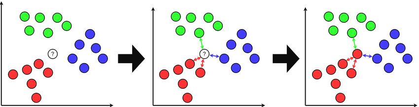
3.1 Bloodhounds Input

The kind of input that Bloodhound will work with will be structured something like
figure 3.1 where each data point shows which files have been touched by a commit
and their current code metric trends. Each time a file have been touched by a commit
it gains a new set of metric values, which with previously values creates code metric
trends. For example, file 3 at commit 3 shows the code metric trends after that file 3 has
been touched 3 times. The goal for Bloodhound is to find a noticeable code metric trend
difference between files that contain bugs (as file 1 and 4) and files that do not contain
bugs (files 2 and 3). For example, if the metric X in figure 3.1 represents number of lines
of code in the file. Then the graph shows a trend that the lines of code increases before a
bug fix commit, but such a trend are not present for commits that are not preceding a bug

                                           13

14                                                            CHAPTER 3. METHOD

fix commit. By finding correlations between code metric trends and bug fix commits,
the classifier should be able to predict bugs.

                             Figure 3.1: Code metric trends

3.2 Design Overview
The design of Bloodhound is visible in figure 3.2. The input is gathered from two places:
cdbs and GitHub. Cdbs provides the code trend metric for the files that have changed
and which commits they were present in. GitHub provides which commits are a part of
a bug fix, though the data from GitHub will be gathered manually from their webpage.
Together, they provide all the data Bloodhound needs. The output Bloodhound provides
to the user are data to evaluate the model and the classification model.
     Because optimization of Bloodhound was outside the scope of this thesis, Blood-
hound was run on a virtual machine in the cloud. So that Bloodhound would have

3.3. CODE TREND METRIC EXTRACTION                                                      15

                            Figure 3.2: Design Bloodhound

access to a computer that could run for a long time uninterrupted. The cloud service
chosen for the task was Google cloud because it gave 3 months of free trial; enough
time for this thesis.

3.3 Code Trend Metric Extraction

For Bloodhound to make its prediction, it needs to get code metric trends of files that
have been changed (part of a commit), in a specific time-frame, for a program. For that
task, cdbs is a fitting tool. Cdbs extracts the code metrics from a program and puts the
extracted data in a MongoDB database, which Bloodhound can access. Bloodhound can
make predictions from every program that cdbs can get code metrics from, but because
cdbs has only been properly tested to extract data from JabRef, Bloodhound will only
be trained with data from JabRef for this thesis. To run cdbs, it needs to get a git
repository, a start date and an end date. Once cdbs has received the necessary input, it
fetches all commits from the GitHub repository that was committed between said dates.
With each commit, an object is created that contains all files and classes that the project
contain. The commit object also contains a list of all files that were changed by the
commit and commit information like date and commit ID. Once a commit object has
been fetched and saved to a database, cdbs begins SonarQube calculations. SonarQube
measures and calculates metrics for each file for each commit and stores them in the

16                                                            CHAPTER 3. METHOD

commit object. Once cdbs have calculated all metrics and stored them in a MongoDB
database, Bloodhound can access the code metrics with the library PyMongo.
     Bloodhound goes through each commit and gathers all .java files that were changed
for that commit. Each files ID are stored in a list in Bloodhound. Then for each file
that has been changed, Bloodhound will look through cdbs data to find which commits
that file were changed, and which metrics values it got. To choose good metrics from
cdbs, they need to correlate with bugs and not depend on each other. Primarily, a lot of
the metrics from cdbs does depend on size. So to avoid size bias, the number of issues
(code smell and vulnerabilities) and complexity is divided on the size of the code. The
metric that Bloodhound gathered from is listed in table 3.1, were the first column shows
the metrics that Bloodhound will generate. The second column a short description of
the metric and the third column which SonarQube metrics from cdbs that Bloodhounds
metrics were generated from.
     After the metric extraction, Bloodhound has a list of 2d matrices, where each matrix
contains the metric values for all commits that a file was touched by. With that, Blood-
hound has the code metric trends for the different files; but at this stage, not which file
or commit is a part of a bug fix.

3.4 Bug Fix Commit Extraction

To find which of the commits from cdbs are a part of a bug fix or not, one needs to
look at bug issues stored on the repositories GitHub page. The bug issues do often
contain a reference to the commits that fixed the bug, which in turn contains the commit
ID. This process can probably be automated with GitHub’s API, with the use of the
command get_issues() to access a repository’s entire issues section [22]. But the process
to automate works as best if the repositories are consistent in where they reference the
bug fix.

3.4. BUG FIX COMMIT EXTRACTION                                                      17

                       Table 3.1: Code metrics for Bloodhound

 Code Metric         Description                             SonarQube Metrics
                     Cyclomatic complexity calculated        complexity/
 complexity
                     by dividing complexity by code_lines    ncloc
                     Density of code smell issues.           code_smell/
 code_smell
                     Higher value means a higher density     ncloc
                     Percentage of all                       comment_lines_density
 comments
                     lines that are comments
                     Density of vulnerabilities issues.      vulnerabilities/
 vulnerabilities
                     Higher value means a higher density     ncloc
                     The mean value of how many              functions/
 avg_len_function
                     lines of code each function contain     ncloc
                     How many lines of code                  ncloc
 code_lines
                     the program has

   In JabRef’s bug issues from 2015 (when JabRef where created) to the end of 2016,
the bug fix commits were found in four places: a merge issue mentioned in the com-
ments, a commit ID mentioned in a comment, a commit ID mentioned in the closing
statement or/and as a milestone. If the bug fix commit were mentioned in the closing
statement/statements or as a milestone then it is straightforward and easy to automate.
And even though not all commits ID mentioned in comments is a bug fix, a clear
majority of them are a bug fix. So even if a few non-bug fix commits were interpreting
as a bug fix commit by the model, they would be probably few enough to not have a
large impact on the model.
   However, the largest problem is the merge issues. In the best case, the merge
issue that did solve the bug issue, were primarily about solving that bug. Nevertheless
sometimes, like bug issue 316, a bug gets solved by a merge issue whose primary goal is
refactoring; or as bug issue 184 that got solved by a merge issue whose primary goal is
to refine a feature. These merge issues can contain many commits, where most of them
do not solve any bugs. Also, it is usually not clear which of the commits that solved
the bug. It might be possible to avoid most of these kinds of merge issues by ignoring

18                                                              CHAPTER 3. METHOD

all merge issues of a specific size. An automation that looks at these four places and
avoids large merge issues might work for JabRef between 2015 and 2016, but there
are no guaranties that it will work for any other repository or even newer versions of
JabRef. Because it might be that such automation might miss bug fix commits if they
are more common in a place that the automation does not look, such as large merge
issues. But the automation might also label non-bug fix commits as bug fixes. If for
example it is common for small non bug fix merge issues, or if non-bug fix commits are
mentioned more in the comments. Because of this, automation will probably need to be
made specifically for one repository, which needs to have clear guidelines on how bug
fix commits should be labelled.
     By manually gathering bug fix commits, a list of bug fix commit ID’s was provided
to Bloodhound. Bloodhound then uses this list to check the commit ID’s from cdbs, to
mark the commit ID as a bug fix or not.

3.5 Classifier Training and Evaluation

To implement a classifier, the library Scikit-learn were used because it is a rich library
with a lot of functions for preprocessing, training and evaluation of classifiers. But to
use Scikit-learn for the classifier, the time series needs to be reinterpreted as a primitive
value, for Bloodhound case a slope. The slope where calculated with the function
stats.linregress from the library SciPy. Before the slope is calculated, the data for a
file contains all the code metric values at every commit the file was touched by, but also
if that commit was a bug fix. The list of commits for each code metric are put in a list
and used as an input to stats.linregress, to generate the overall slope for that particular
code metric. This is done for each code metric. With this each files code trend metric
can be represented as a list, where the last element tells if the list were part of a bug
fix. So as seen in figure 3.3, the data is converted from a list of files, where each file is

3.5. CLASSIFIER TRAINING AND EVALUATION                                               19

represented as a matrix, to one matrix where each row represents a file.

                        Figure 3.3: Preprocessing for the model

   For distance based classifiers such as K-NN the metrics needs to have a similar
scale, which is achieved with feature scaling. Without it, the classifier could get a bias
for or against metrics dependent on the metrics scales [23]. Bloodhound implements
feature scaling with the Scikit-learn function MinMaxScaler which will put all metrics
on a scale from 0 to 1 [24].
   To split the data for training and testing, k fold cross validation is used with the
function KFold. To choose a good k value for k fold cross-validation, the research “The
K in K-fold Cross Validation” found that an optimal k-value depends on the data, but in
general, a k value of four performs well [25]. Also, the function KFold uses 5 as default
[26], therefore k were kept as 5. The classifier is then trained with the algorithm K-NN,
with the training data from k fold cross validation. To choose a good k value for K-NN,
the paper “Do we need whatever more than K-NN?” found the best prediction got when
k was between 10 and 20 [16]. To make sure that the best k-value are chosen, k will
be tested with the odd numbers from 1 to 23 or until the model stops predicting bugs or
non-bugs.
   To evaluate how good the model are, values for tp(true positive), fp(false posi-
tive), fn(false negative) and tn(true negative) were gathered with the function confu-
sion_matrix from the library Scikit-learn. With them, five metrics where be calculated,
precision, recall, specificity, accuracy and f1 -score. Precision shows how many of
the bug predictions that were correct. Recall how many of the bugs that were found.

20                                                                  CHAPTER 3. METHOD

Specificity how many of the non-bugs that were found. Accuracy, how many of the
predictions (both bug and non-bug) were correct. And lastly f1 -score, which merges the
precision and recall to one score so that it gets easy to point out which k value for K-NN
performs the best bug prediction. [27]

                                              tp
                            precision =
                                          tp+ f p
                                              tp
                                 recall =
                                          tp+ fn
                                              tn
                           specificity =
                                          tn + f p
                                                 t p + tn
                            accuracy =
                                          t p + tn + f p + f n
                                               precision · recall
                             f1 -score = 2 ·
                                              precision + recall

3.6 Summary
With code trend metrics gathered from cdbs and bugs fix commits gathered from GitHub,
Bloodhound has data to train a classification model that predicts bugs in a program. Data
for evaluation and the classification model are accessible to the user.

Chapter 4

Results

Within this chapter the result and evaluations of this thesis will be presented. The Result
and evaluation will include a description of the workings of Bloodhound, information
from the development, how Bloodhound’s performance relates to similar and related
work.

4.1 Evaluation

4.1.1 Evaluation Setting

For this project the system JabRef was analysed. The commits which data was extracted
from, came from 2016 between commit 2d04b6c5bf1fd582a57e5e67a9f6c4cc7ca37228
on June 1 and commit 304d2802162a7e75edda5fbc893666cc73efe669 on July 13 (42
days). The repository contained 202 commits between these dates. Of them, 45 commits
were a bug fix. 312 classes were touched during the time frame, of them 37 were touched
by a bug fix commit.

                                            21

22                                                            CHAPTER 4. RESULTS

4.1.2 Evaluation Results

The graph 4.1 shows the compressed result of testing different k values for K-NN, where
the full output can be found in appendix A. Every odd number between 1 and 13 were
tested. Higher k-values were not tested because from the k value 9, Bloodhound started
predicting that all files were bug-free. At 5-NN were the highest F1 -score achieved, with
a recall of 25% and precision of 42%.

                             Figure 4.1: Model evaluation

4.1.3 Discussion of Evaluation Results

At the highest F1 -score with the classifier 5-NN, the accuracy was high, but the metrics
of the bug predictions was quite low. Which shows that the tool is not performing well.
A study made by a team from the University of Szeged [19] shows that by using ML
algorithms and software metrics could identify 61% of classes with bugs. The study
used a total of 47 618 commits, 5360 out of the 8780 classes with bugs was identified
and 5255 classes amongst the 38 838 classes that did not contain bugs was predicted to
contain bugs. This would mean that the precision would be 50.49%, recall 61.05% and
accuracy 83.99%. The project from [21] that also uses software metrics and a variety

4.2. PROBLEMS AND ISSUES                                                              23

of ML algorithms produced an average recall of 69% and a precision of 63%. These
numbers are not optimal and so neither of the tools performed without flaws. This does
however show that the Bloodhound tool did not perform as well as it could have done
with the low recall of 25% and precision of 42%.
   An alternative to using software metrics as predictors to Bloodhound the study [20]
performed bug prediction by using pre-processed datasets. Once three different datasets
had been used for prediction, the tool achieved a recall of 98.3% and 98.8% precision.
These percentages are significantly higher than those of both Bloodhound and related
projects which uses software metrics and therefore shows great potential.
   One aspect that might be the reason for the tools low performance is that a relatively
low amount of commits were used. The tool cdbs that provides Bloodhound with metric
data can extract metric data from a time-frame of 2 years with over 3000 commits.
Unfortunately, cdbs started malfunctioning close to the end of the project when the full
time-frame was to be analysed. This meant that the only metric data that could be used
for the final analysis was the small portion that had been used during development for
fast testing. With this small amount of data, each class that was analysed was only
changed 1.47 times on average which meant that the trends could either not be analysed
or contain a small amount of useful data.

4.2 Problems and Issues

4.2.1 Cdbs

Without the use of Schulte’s tool cdbs this project would most likely not have been able
to happen within the available time span. By using Schulte’s tool, SonarQube calcula-
tions was able to be used and extracted as matrices without the need of implementation.
This saved the project a large amount of time and made sure that all the data that the
project would need was accessible from the beginning.

24                                                             CHAPTER 4. RESULTS

     Even though Schulte’s tool has helped the project in many ways, the usage of the
tool has not always been easy due to a variety of reasons. Among these reasons is the
fact that the tool has to run for five days in order to calculate all data from two years of
commits. Which means that usage of the computer that is running the tool is drastically
restricted due to CPU usage. Another reason would be that the tool was produced to
answer a specific thesis and is not made to be used for a variety of tasks. This means
that the tool is not perfect and will have to be tweaked to fit the task and therefore
requires some insight to the workings of the tool.
     In general, the tool has provided a substantial amount of help. And even though there
has been issues, Schulte has provided support via both email and meetings whenever an
issue has appeared.

4.2.2 Cloud Computing

Due to the high CPU usage of both Bloodhound and cdbs development, testing and
the running of the project was done on a virtual machine on Google’s cloud computing
services. The issue that appeared with this solution was that in order to save money on
the project, the free period that all users receive was to be used. Rehnholm had already
used his free period for a previous project and so Rysjö’s free period had to be used.
When Rysjö was starting his free period, issues with registration appeared and support
was contacted. Due to the support team at Google not being able to find a solution,
the back-and-forth communication between Rysjö and the support team meant that the
development and implementation was held up.
     After some time, the issue was resolved and the development could officially start.
During the time spent on troubleshooting, development was done too as good of an
extent as possible without a designated machine. Even with the parallel work that was
done while handling the issue. The issue itself caused the project’s development to slow
down significantly before the issue was solved.

4.3. SUMMARY                                                                       25

4.3 Summary
Bloodhound’s result are too weak for predicting bugs, but because other related work
has shown a better result, there are still potential for bug predictions with ML. This
thesis has also shown the difficulties of using software developed for a single user to
solve a specific task. This challenge can however be more than possible by keeping
constant and proficient contact with the software developer of said software.

26   CHAPTER 4. RESULTS

Chapter 5

Conclusions

This thesis purpose is to explore the possibilities to predict bugs with TSC of code
metric trend. It can be hard to tell how good a classifier must be to be seen as successful
in its task of predicting bugs, but in comparison with similar research, Bloodhound has
a low performance. While Bloodhound got a recall of 25% and precision of 42%, other
research has achieved a precision and recall over 50%. The bad result is most likely
because Bloodhound were trained on a too short time-frame, so that the files did not
change enough for a noticeable trend to emerge.
   The first thing that one could do to achieve better results from Bloodhound is to
train Bloodhound on a longer time-frame, like a year. The next step would be to test
if removing commits after a bug fix would achieve better predictions. So that the code
metric trend for bug files only contains commits with bugs. After that, it would be
good to test different algorithms, which should be relative easy to implement if one uses
implementations from Scikit-learn. By testing different algorithms and comparing their
results, one could find the most efficient algorithm for Bloodhound.
   If after all this Bloodhound still gets bad predictions, or that the kind of prediction it
gives is not useful. One could use a library like sktime that does not need to reinterpret
the time-serie as a primitive value. But before trying to implement sktime, one needs to

                                            27

28                                                     CHAPTER 5. CONCLUSIONS

make sure that the bugs related to distance based classifiers are solved.

Bibliography

[1] celerity. The true cost of a software bug: Part one. https://www.celerity.
   com/the-true-cost-of-a-software-bug. url date: 2021-05-11.

[2] Edith Tom, Aybüke Aurum, and Richard Vidgen.                An exploration of
   technical debt. https://www.sciencedirect.com/science/article/pii/
   S0164121213000022, December 2012. url date: 2021-05-04.

[3] Daniela Steidl, Florian Deissenboeck, Martin Poehlmann, Robert Heinke,
   and Bäarbel Uhink-Mergenthaler.          Continuous software quality control in
   practice. https://www.cqse.eu/fileadmin/content/news/publications/
   2014-continuous-software-quality-control-in-practice.pdf,                  2014.
   url date: 2021-05-04.

[4] Foutse Khomh, Massimiliano Di Penta, Yann-Gaël Guéhéneuc, and Giuliano
   Antoniol. An exploratory study of the impact of antipatterns on class change- and
   fault-proneness.   https://swat.polymtl.ca/~foutsekh/docs/Prop-EMSE.
   pdf. url date: 2021-06-08.

[5] Wei Li and Raed Shatnawi. An empirical study of the bad smells and class error
   probability in the post-release object-oriented system evolution. https://www.
   sciencedirect.com/science/article/pii/S0164121206002780. url date:
   2021-06-08.

                                       29

30                                                               BIBLIOGRAPHY

 [6] Moritz Schulte Lukas. Analyzing dependencies between software architectural
     degradation and code complexity trends. Master’s thesis, Karlstads University,
     2021.

 [7] Aline Lopes Timóteo, Alexandre Álvaro, Eduardo Santana de Almeida,
     and Silvio Romero de Lemos Meira.             Software metrics:    A survey.
     https://citeseerx.ist.psu.edu/viewdoc/download;jsessionid=
     E6128384FCF754575B86BDA5AF91D873?doi=10.1.1.544.2164&rep=rep1&
     type=pdf. url date: 2021-05-11.

 [8] Intetics. The 3 types of metrics to assure software quality. https://intetics.
     com/blog/3-types-of-metrics-software-quality-assurance-2.                  url
     date: 2021-05-12.

 [9] Sonar Qube.      Document 8.7.      https://docs.sonarqube.org/latest/
     user-guide/metric-definitions/. url date: 2021-03-04.

[10] Qiong Liu and Ying Wu. Supervised learning. https://www.researchgate.
     net/publication/229031588_Supervised_Learning, January 2012. url date:
     2021-05-12.

[11] D. Michie, D.J. Spiegelhalter, and C.C. Taylor. Machine learning, neural and
     statistical classification. http://ambio1.leeds.ac.uk/~charles/statlog/
     whole.pdf, February 1994. url date: 2021-05-12.

[12] Bagnell Anthony, Bostrom Aaron, and Lines Jason.             The great time
     series classification bake off:     An experimental evaluation of recently
     proposed algorithms. extended version.    https://www.researchgate.net/
     publication/301856632_The_Great_Time_Series_Classification_
     Bake_Off_An_Experimental_Evaluation_of_Recently_Proposed_
     Algorithms_Extended_Version, February 2016. url date: 2021-01-27.

BIBLIOGRAPHY                                                                        31

[13] Xi     Xiaopeng,       Keogh        Eamonn,        Shelton    Christian,      and
    Wei     Li.          Fast     time   series    classification   using     numerosity
    reduction.                  https://dl.acm.org/doi/abs/10.1145/1143844.
    1143974?casa_token=43laLCbv-CkAAAAA:TZuz1RX9ecyDUZC1_
    XW6S2k9Iws55IaakNdBTuqT21Zpny1TnubNPVVnEWlDSFVK4GJlbRXU_Q,                    June
    2006. url date: 2021-01-28.

[14] Ding Hui, Trajcevski Goce, Scheuermann Peter, Wang Xiaoyue, and Keogh
    Eamonn. Querying and mining of time series data: Experimental comparison
    of representations and distance measures.             https://dl.acm.org/doi/
    abs/10.14778/1454159.1454226?casa_token=jQQkAkJ9uXEAAAAA:
    HHd-hC0LMXPNRWEpxaYVgj9aCfdEzE5pvJ6KCMA4noMH6xAHUh2BoDf2vasnIWIyNy2SAYPFug,
    August 2008. url date: 2021-01-28.

[15] J. Berndt Donald and Clifford James.         Using dynamic time warping to find
    patterns in time series. https://www.aaai.org/Library/Workshops/1994/
    ws94-03-031.php, April 1994. url date: 2021-01-29.

[16] Kordos Miroslaw and Blachnik Marcin.           Do we need whatever more than
    k-nn?     https://www.researchgate.net/publication/226719726_Do_We_
    Need_Whatever_More_Than_k-NN, January 1970. url date: 2021-04-28.

[17] Karim Fazle,     Majumdar Somshubra,          Darabi Houshang,        and Harford
    Samuel.       Multivariate lstm-fcns for time series classification.         https:
    //www.sciencedirect.com/science/article/pii/S0893608019301200?
    casa_token=vDMVvUY4q3oAAAAA:5Cam28Xtx4nn5FCg4_
    0fSEXIazXm37wsw0Rb7eBhGOQ9XNCJu3NM1ZIXArmIeWcRBZcOw-M,                        April
    2019. url date: 2021-02-11.

32                                                                BIBLIOGRAPHY

[18] CodeScene.    The next generation of code analysis, predictive and powerful.
     https://codescene.com/how-it-works/. url date: 2021-04-21.

[19] Tamás Grósz Tibor Gyimóthy Rudolf Ferenc, Dénes Bán. Deep learning in static,
     metric-based bug prediction.    https://www.sciencedirect.com/science/
     article/pii/S2590005620300060#!, 2020. url date: 2021-05-04.

[20] Awni Hammouri, Mustafa Hammad, Mohammad Alnabhan, and Fatima
     Alsarayrah.       Software bug prediction using machine learning approach.
     International Journal of Advanced Computer Science and Applications,
     9(2),   january     2018.       https://pdfs.semanticscholar.org/a5f6/
     5fe00bf4b467e6166487f0c2ffc4b66d9593.pdf.

[21] Wasiur Rhmann, Babita Pandey, Gufran Ansari, and D.K.Pandey. Software fault
     prediction based on change metrics using hybrid algorithms: An empirical study.
     Journal of King Saud University - Computer and Information Sciences, 32(4):419–
     424, December 2018. https://www.sciencedirect.com/science/article/
     pii/S1319157818313077#f0005.

[22] Emily Riederer. projmgr: Task tracking and project management with github.
     https://rdrr.io/cran/projmgr/. url date: 2021-05-04.

[23] scikit-learn developers.       Importance of feature scaling.          https:
     //scikit-learn.org/stable/auto_examples/preprocessing/plot_
     scaling_importance.html. url date: 2021-06-05.

[24] scikit-learn developers.       sklearn.preprocessing.minmaxscaler.     https:
     //scikit-learn.org/stable/modules/generated/sklearn.
     preprocessing.MinMaxScaler.html. url date: 2021-06-05.

[25] Anguita Davide, Ghelardoni Luca, Ghio Alessandro, Oneto Luca, and Ridella

BIBLIOGRAPHY                                                                           33

     Sandro. The k in k-fold cross validation. https://www.elen.ucl.ac.be/
     Proceedings/esann/esannpdf/es2012-62.pdf, 2012. url date: 2021-04-26.

[26] scikit-learn developers. sklearn.model selection.kfold. https://scikit-learn.
     org/stable/modules/generated/sklearn.model_selection.KFold.html.
     url date: 2021-05-09.

[27] scikit-learn developers. 3.3. metrics and scoring: quantifying the quality of predic-
     tions.   https://scikit-learn.org/stable/modules/model_evaluation.
     html. url date: 2021-06-05.

34   BIBLIOGRAPHY

Appendix

   35

Appendix A

Results from Bloodhound

              Figure A.1: 1-NN

              Figure A.2: 3-NN

              Figure A.3: 5-NN

                    37

38   APPENDIX A. RESULTS FROM BLOODHOUND

     Figure A.4: 7-NN

     Figure A.5: 11-NN

     Figure A.6: 13-NN