Bumble bee species distributions and habitat associations in the Midwestern USA, a region of declining diversity
←
→
Page content transcription
If your browser does not render page correctly, please read the page content below
Biodiversity and Conservation (2021) 30:865–887
https://doi.org/10.1007/s10531-021-02121-x

ORIGINAL PAPER

Bumble bee species distributions and habitat associations
in the Midwestern USA, a region of declining diversity

Jessie Lanterman Novotny1,3 · Paige Reeher2,4 · Megan Varvaro1 ·
Andrew Lybbert1,5 · Jesse Smith2,6 · Randall J. Mitchell2 · Karen Goodell1

Received: 8 July 2020 / Revised: 30 December 2020 / Accepted: 10 January 2021 /
Published online: 7 February 2021
© The Author(s) 2021

Abstract
Bumble bees (Bombus spp.) are important pollinators, yet rapidly declining globally. In
North America some species are thriving while others are nearing extinction. Recognizing
subtle differences in species’ biology and responses to environmental factors is required to
illuminate key threats and to understand their different population trajectories. We inten-
sively surveyed bumble bees in Ohio, USA, along the receding southern boundary of many
species’ ranges, to evaluate current conservation status of the state’s species. In 318 90-min
field surveys across two consecutive years we observed 23,324 bumble bees of 10 species
visiting 170 plant species. Habitat, landscape, latitude, and their interactions significantly
influenced bumble bee abundance, species richness, and community composition during
peak season. Sites planted with flowers yielded more bumble bee individuals and species
than did sites not planted with bee food plants. Bombus impatiens, B. griseocollis, and B.
bimaculatus comprised 93% of all observations. Their abundances all peaked in habitats
planted with wildflowers, but there were species-specific responses to local and landscape
factors. Three less common species (B. fervidus, B. vagans, and B. perplexus) were more
likely to be found in forested landscapes, particularly in the northeastern portion of the
state. Bombus perplexus was also affiliated with planted urban wildflower patches. These
results provide a strong starting point for future monitoring and conservation interven-
tion that targets less common species. A quantitative synthesis of detailed state-level and
regional datasets would allow additional insight into broad scale patterns of diversity in
bumble bee communities and species conservation trajectories.

Keywords Bombus · Community ecology · Conservation · Landscape ecology · Planted
pollinator habitat · Statewide survey

Communicated by Nigel E. Stork.

* Jessie Lanterman Novotny
  JessieLantermanNovotny@gmail.com
Extended author information available on the last page of the article

                                                                                          13
                                                                                  Vol.:(0123456789)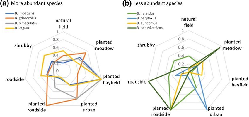
866                                                   Biodiversity and Conservation (2021) 30:865–887

Introduction

Bumble bees (Bombus) are conspicuous eusocial insects that are critically important pol-
linators in both natural and agricultural habitats (Losey and Vaughan 2006; Kremen et al.
2007; Goulson 2010). Though most species are highly generalized foragers, bumble bees
can play unique roles in plant-pollinator interaction networks by using their long tongues
to access flowers with deep corolla tubes, by buzz pollinating flowers, and by prying open
large closed flowers (Macior 1969; Heinrich 1976; Russell et al. 2017). Evidence indicates
that bumble bees are declining over broad areas of the globe (Goulson et al. 2008; Cam-
eron and Sadd 2020), including in North America (Grixti et al. 2009; Cameron et al. 2011;
Colla et al. 2012). The erosion of bee diversity, in general, is associated with increased
food stress from reduced floral diversity, continuing habitat loss, increased pesticide use,
and disease (Cameron et al. 2011, 2016; Goulson et al. 2015). However, some species of
bumble bees have suffered greater losses than others (Cameron and Sadd 2020). Among
North American species there are many questions, but few answers, as to why some species
appear to be thriving and others nearing extinction. Subtle differences in phenology, habi-
tat use, diet breadth, nesting behavior, and responses to environmental stressors of North
American bumble bee species may contribute to their current status and differing popu-
lation trajectories (Williams et al. 2009; Williams and Osborne 2009; Wood et al. 2019;
Liczner and Colla 2020). Baseline information on current abundances and distributions are
uneven and incomplete, especially for North American species (Colla and Packer 2008;
Richardson et al. 2019; Wood et al. 2019). In this study we focus on Midwestern USA
bumble bee fauna habitat affiliation and environmental drivers of community structure.
    Conservation of bumble bees depends on a strong understanding of both the natural
and anthropogenic factors that determine the availability of key resources (Roulston and
Goodell 2011; Cariveau and Winfree 2015), and these factors are likely to act on a range of
spatial scales. At the local level bees can respond directly to the availability of suitable for-
aging, nesting, and overwintering sites in different habitats (Carvell et al. 2011; Lanterman
et al. 2019). At the landscape level they respond to the mosaic of suitable habitats in the
surrounding area (at a scale of several kilometers) and the quality of the intervening matrix
that determines their connectivity (Hines and Hendrix 2005; McFrederick and LeBuhn
2006; Heard et al. 2007; Ahrné et al. 2009; Ropars et al. 2020). At the regional level, pres-
ence of bumble bee species may vary with latitude, altitude, and other large-scale features
that determine whether a location lies within the physiological tolerance of each species
(Hines 2008; Dohzono and Suzuki 2010; Williams et al. 2014). Bumble bee communities
can be shaped further by competition, predation, pathogens, floral hosts, and restoration
and management activities (Goulson 2010). Biological differences among species interact
with these environmental factors to influence their distribution, abundance, and susceptibil-
ity to population declines (Schochet et al. 2016).
    The state of Ohio is situated at the convergence of the Midwestern and the Northeastern
regions of the United States. A total of 54% of Ohio’s land is farmed (USDA 2019), includ-
ing crops that benefit from bumble bee pollination services (Park et al. 2016; McGrady
et al. 2020). Of the twenty species of bumble bee historically documented in Ohio, only
half of them have been seen regularly in the last century (Lanterman et al. 2019). Bom-
bus affinis, listed as endangered on the IUCN Red List in 2015 (Hatfield et al. 2015) and
federally endangered in 2017 (Christopher 2016), was last seen in Ohio in 2013 (speci-
men vouchered at the Toledo Zoo); B. terricola, federally identified as a species of concern
in 2016, has not been recorded in the state since 1981 (specimen vouchered at the Ohio

13
Biodiversity and Conservation (2021) 30:865–887 867
State University C.A. Triplehorn Collection). However, both can still be found in nearby
states. Furthermore, many North American Bombus have a southern range margin in or
near Ohio (Colla et al. 2011). Lower latitude boundaries appear to be shifting northward,
and ranges are contracting for many northern hemisphere Bombus species in response to a
changing climate (Kerr et al. 2015). Therefore, Ohio is well positioned to study changes in
bumble bee species distributions and community composition along the southern boundary
in the northcentral and eastern USA. Deeper knowledge of species distributions and habi-
tat associations in Ohio may illuminate key threats, help identify strategies to slow losses
of declining species, and predict future vulnerability of currently stable species (Williams
et al. 2009; Kerr et al. 2015).
The burgeoning initiatives to conserve, improve, and construct pollinator habitat will
benefit from solid bumble bee distribution data on multiple spatial scales. Rigorous data-
sets on bumble bee species’ habitat affinities will allow local habitat managers to target
at-risk species and evaluate which interventions most effectively promote those species
(Liczner and Colla 2020). To date, however, no studies have thoroughly documented the
distribution and abundance of Bombus across the state of Ohio, nor have any studies inves-
tigated species-specific habitat and landscape associations that might explain variation in
their distribution. Because the majority of species found in midwestern North America
have low relative abundances (Preston 1948), intensive sampling is required to generate
data sets large enough to evaluate patterns of the distribution and abundance of less com-
mon species (Cameron et al. 2011).
We conducted a comprehensive two-year survey of bumble bees in Ohio to document
their current abundance, distribution, habitat use, and response to various environmental
factors. We aimed to sample intensively enough to not only document general drivers of
bumble bee abundance and diversity, but to discern species-specific patterns of habitat
use. We addressed the following questions: How are bumble bee diversity, abundance, and
community composition affected by local flower availability and landscape context? How
do species differ in their habitat associations? Are there geographical or latitudinal patterns
in species occurrence or relative abundance across the state of Ohio?
Methods
Study sites
We conducted 318 90-min surveys of bumble bees (Bombus spp.) and wildflowers
at 228 locations in Ohio, U.S.A, between June and August 2017 and 2018. Study sites
consisted of flower-rich patches of foraging habitat greater than 0.4 ha (mean 9.0 ± 15.2,
max 134.4 ha) that were at least 2 km apart, and included public lands (n = 198), roadside
patches of wildflowers (n = 41), private nature preserves (n = 49), and private residential
properties (n = 30). Sites were classified into the following habitat categories based on their
dominant vegetation and management history: natural field, shrubby successional old field,
planted hayfield, planted restored meadow, planted urban patch, planted restored roadside,
or roadside (Electronic Supplementary Material, Table S1). Planted sites included pollina-
tor-friendly and native prairie wildflower species. The extent of suitable foraging habitat
at each site was first ground truthed during field surveys and later digitized using Google
Earth software.
13868 Biodiversity and Conservation (2021) 30:865–887 Bee field surveys We based our sampling design on Ward et al. (2014) and the US Fish and Wildlife B. affinis survey protocol (2017). Bee surveys were performed between the hours of 0900 and 1800 on days without precipitation, with little or no wind, and with air temperature above 21 °C. Upon each site visit, a team of one to four trained observers recorded bee visits to flowers for a total of 90 person minutes, not including netting and handling time. If there was one observer, that person netted for the full 90 min. If two observ- ers were present, each netted independently for 45 min. For three or four observers, the time per person was reduced accordingly. The observers spread out and walked slowly through the best available foraging habitat, recording all bee visits to flowers and the flower species on which they were observed. We recorded species identity and social caste of each bumble bee. Bumble bees were either identified to species on the wing, or were netted, identified using a field guide (Colla et al. 2011), photographed if needed for identification confirmation, and re-released on site. To minimize our impact and because of the large number of bumble bees observed at some sites (as many as 452 in a single 90-min survey), the majority of bees were not collected. We searched systematically, moving between flower patches often, to minimize double-counting of individual bees. Plant field surveys We estimated the available flower resources for bees at each site on every visit by sur- veying flowers along four 25 m by 1 m transects (100 m2 total area). The four tran- sects were placed within the site in a way that represented the flower community in the area where bees were surveyed. For instance, if we had surveyed flowers along the forest edge, within mowed paths, and in open field, we would haphazardly place tran- sects within each of these areas to capture the primary floral resources used by bumble bees, choosing areas roughly based on the amount of time we spent surveying each. In each transect, we recorded the number of flower units of each species in bloom. Spe- cies that exceeded 1000 flower units per 25 m transect were recorded as “1000.” Flower units were defined in “bee walkable clusters,” with one unit as the number of flowers a bee could visit by walking before it would have to fly to the next cluster (Saville 1993). What constituted a flower unit was defined separately for each plant species (but con- sistently across all observers), based on floral morphology and on observations of bee foraging behavior. Plant species were identified using a field guide (Newcomb 1989) or were photographed for later identification. Landscape assessment To evaluate the landscape around each site, we used remotely-sensed data to calculate the proportion of forest (deciduous and conifer), shrub, fields (alfalfa, clover, other hay, idle cropland, grassland, pasture, and developed open space), developed areas (low, medium, and high intensity), wetlands (woody and emergent herbaceous), pollinator- supporting crops (fruits and vegetables that flower before harvest), and non-pollinator- supporting crops (grains, tree crops, sod-grass, and other crops that are harvested before flowering) using ArcGIS software (ESRI 2016). This simplified land cover classification scheme was modified from the USDA Cropland Data Layer (CDL 2018 version; USDA 13
Biodiversity and Conservation (2021) 30:865–887 869
2019). We considered landscape composition at three spatial scales—a 1.0-km, 1.5-km,
and 2.0-km buffer radius areas from the geographic site centroid—based on bumble
bee foraging distances reported in the literature (Dramstad 1996; Osborne et al. 1999;
Walther-Hellwig and Frankl 2000a, b; Wood et al. 2015). We used generalized linear
models and AICc values to determine that the 2.0-km landscape scale better reflected
variation in Bombus abundance and richness.
Data analysis
We restricted our flower richness and abundance measures to only include flower species
that were visited by at least one bee during our surveys. For most analyses, we grouped
two morphologically similar bumble bee species—B. auricomus and B. pensylvanicus—
because not all were distinguished in the field, and they accounted for a low proportion of
observations in any given survey. Two rare species in our dataset—B. citrinus (3 individu-
als observed) and B. borealis (a single individual)—were retained for abundance and rich-
ness analyses but omitted from community ordination to avoid their disproportionate influ-
ence on pairwise distances among sites and ordination configuration (McCune et al. 2002).
Abundance data were natural log transformed as needed to improve their fit to a Gaussian
distribution. To assess differences in bee diversity between sites, independently of abun-
dance, data were rarefied down to 19 bumble bees per survey and the average species rich-
ness of 1000 random bootstrap replicates was calculated (rrarefy function, ‘vegan’ pack-
age). Fifty surveys in which fewer than 20 bumble bees were found were excluded from
rarefaction analysis. We were able to visit a minority of sites twice, but they were visited in
different years and different times, so due to high background variation in bee survey yield
they were treated as independent observations. Most analyses were conducted using R, ver-
sion 3.5.3 (R Development Core team 2019). JMP software version 14 (2018) was used to
construct generalized linear models with logit link functions on presence/absence data for
rarer species.
We used multiple regression models to evaluate how habitat, flower resources, landscape,
and time of season affected overall bumble bee abundance and diversity in our surveys. To
investigate whether common species responded differently to environmental features, mod-
els were also constructed separately for each of the three most abundant species. Models of
bumble bee abundance and raw and rarefied species richness were fitted with the following
potential main effects: growing degree day (GDD; determined using the online calculator at
https://www.oardc.ohio-state.edu/gdd/default.asp), latitude, flower abundance, flowering spe-
cies richness, habitat type, and the proportion of forest (hereafter “forest”) and urban devel-
oped area (hereafter “developed”) in the landscape. We also included the two-way interaction
terms between habitat and all local and landscape level variables that have been shown to
modify the quality of a specific habitat for bumble bees (e.g., Ahrné et al. 2009, Cariveau
and Winfree 2015; Carvell et al. 2011; Heard et al. 2007; Hines 2005; Lanterman et al 2019;
Reeher et al. 2020; Schochet et al. 2016), as well as GDD, which helps account for phenologi-
cal effects on bumble abundance and richness (Lanterman et al 2019). Finally, we included a
flower abundance x flower richness interaction to help account for the overall availability of
flower resources. A gaussian distribution was selected for each response variable based on
the model adjusted R2 values under different distributions and Shapiro tests for normality of
model residuals. Prior to model construction, we checked for collinearity of continuous pre-
dictor variables by calculating a Pearson correlation matrix. There was a moderate negative
correlation between developed land and forest (Pearson r = -0.53); all others were less than
13870 Biodiversity and Conservation (2021) 30:865–887
0.5. Continuous predictor variables were standardized and centered by subtracting the mean
from each observation then dividing by the standard deviation. For each model, we calculated
Variance Inflation Factors (VIFs) for each independent variable and found no evidence of
multicollinearity. To compare the amount of variance explained by each factor or interaction
in our models, we calculated their partial eta-squared values (Richardson 2011). We used the
Tukey procedure for pairwise contrasts of mean abundance and richness between all habitat
types within the model framework (package ‘lsmeans;’ Lenth 2016). Complete model sum-
maries are given in the Electronic Supplementary Material, Tables S2–S7.
We investigated the factors influencing the probability of occurrence of the less common
species (B. fervidus, B. vagans, B. perplexus, B. auricomus, and B. pensylvanicus) using gen-
eralized linear models with a logit link function on presence versus absence data. We focused
these analyses on broad-scale factors because we suspected that the presence/absence data
would be less sensitive than abundance data to snapshot measures of local environmental
quality, such as flower abundance and richness. Therefore, for each of these five species we
analyzed its presence versus absence as a function of habitat type, landscape context, latitude,
and their first-order interactions. We used the Firth adjusted maximum likelihood method to
estimate parameter values. Non-significant terms were dropped from models sequentially,
starting with the lowest likelihood ratio chi square value, and each reduced model was com-
pared to the previous using AICc. For each species we retained the model that had the most
independent variables and an AICc at least 2 lower than the next best fit model. There were
not enough sightings of B. citrinus or B. borealis to analyze.
To visualize bumble bee community composition, we used non-metric multidimensional
scaling (NMDS) ordination (metaMDS function, ‘vegan’ package; Oksanen et al. 2016). We
tested for differences in community composition by habitat type and month using permuta-
tional analysis of variance adonis tests (adonis function, 500 permutations, ‘vegan’ package)
based on Bray–Curtis dissimilarity between sites. To visualize the influence of landscape and
other continuous variables on bee community composition, we fitted significant predictor vec-
tors to the ordination plot using the envfit function in the ‘vegan’ package.
Indicator species analysis was used to determine if bumble bee species were associated
with particular habitat types (indval function, ‘labdsv’ package, 500 iterations; Roberts 2016).
An indicator value was calculated for each species—habitat combination as the product of the
relative frequency and relative average abundance of a species at sites of a particular habitat
type, taking into account the number of sites in that habitat group.
To visualize differences in habitat use by each bumble bee species, we standardized abun-
dance values for the June-July samples by dividing the mean abundance per survey by the
maximum value for that species across habitats. These values were plotted using radar charts.
Bombus auricomus and pensylvanicus were plotted separately for this analysis using the sub-
set of individuals from the B. auricomus/pensylvaniucs morphotype that we had identified to
species with confidence.
Results
In 318 surveys (477 h) we recorded 23,324 bumble bees representing 10 species (Table 1),
visiting 170 flowering plant species. In an average 90-min field survey, we observed
73 ± 65 SD bumble bees (range 2–452) of 3.9 ± 1.2 species (range 1–7).
Three species accounted for 93% of all bumble bee sightings: Bombus impatiens
(50%), B. griseocollis (30%), and B. bimaculatus (14%). These three abundant species
13Table 1 Seasonal variation in the total number of bumble bees (Bombus spp.) observed in field surveys
Species June July August Total
Abundance Proportion of Abundance Proportion of Abundance Proportion of Abundance Proportion
surveys surveys surveys of surveys
B. impatiens 1525 0.90 4860 0.94 5221 1.00 11,606 0.94
Biodiversity and Conservation (2021) 30:865–887
B. griseocollis 2653 0.97 3633 0.95 599 0.81 6885 0.93
B. bimaculatus 1869 0.94 1365 0.80 22 0.22 3256 0.73
B. vagans 226 0.38 297 0.42 108 0.43 631 0.41
B. fervidus 107 0.37 170 0.38 71 0.42 348 0.38
B. auricomus/pensylvanicus 90 0.23 195 0.36 48 0.27 333 0.29
B. perplexus 140 0.21 42 0.15 6 0.04 188 0.15
B. citrinus 3 0.02 0 0.00 0 0.00 3 < 0.01
B. borealis 0 0.00 1 < 0.01 0 0.00 1 < 0.01
B. sp. 34 0.13 33 0.12 6 0.06 73 0.11
Species are listed in order of most to least abundant. B. sp. indicates individuals whose species identity could not be determined. The total counts for each species are given, as
well as the proportion of surveys in which they were observed (out of 112 surveys in June, 138 in July, and 68 in August)
871
13872 Biodiversity and Conservation (2021) 30:865–887 each occurred in over 90% of surveys (Table 1). Bombus vagans and B. fervidus were each found in approximately one-third of all surveys, and B. perplexus in 15% of sur- veys. The nest parasite Bombus citrinus was observed infrequently. A single worker of B. borealis was observed in July in the northeast of the state, apparently the first sighting in Ohio since the 1950s, according to records from the Cleveland Museum of Natural History Insect Collection and the C.A. Triplehorn Insect Collection at the Ohio State University (specimen verified and vouchered at the Cleveland Museum of Natural History). We did not observe two species of particular conservation concern that were historically found in Ohio (B. affinis and B. terricola), despite intensive survey effort and inclusion of suitable habitat in and near locations where they were most recently sighted. Bombus impatiens was the most abundant bumble bee species in half of the surveys (152 out of 318). In a quarter of the surveys (88 out of 318), this species was more than twice as abundant as the next most numerous. Bombus impatiens increasingly domi- nated surveys as the season progressed (accounting for 22% of Bombus sightings in June, 45% in July, and 85% in August, Fig. 1, Table 1; F = 14.37, df = 3, 314, p < 0.01). During late summer surveys bumble bee abundance per survey increased (59 ± 45 bum- ble bees per survey in June, 77 ± 70 in July, 89 ± 78 in August) but diversity declined (4.1 ± 1.2 species in June; 4.0 ± 1.2 in July; 3.2 ± 1.1 in August). Therefore, August sam- ples were excluded from further analyses, and only June and July surveys (peak season for all other bumble bee species) were used in the analyses below. Fig. 1 NMDS ordination of seasonal variation in bumble bee species assemblage (based on Bray–Cur- tis distances, final stress with 3 axes = 0.11, n = 318 surveys). White circles represent June surveys, light gray squares July, and dark gray triangles August (adonis test by month F = 14.37, R2 = 0.12, df = 3, 314, p < 0.01). Black ellipses represent 1 SD areas around group centroids. Black squares show the position of each bumble bee species. Bombus species are abbreviated as follows (top to bottom): B.imp (B. impatiens), B.fer (B. fervidus), B.vag (B. vagans), B.aur/pen (B. auricomus/pensylvanicus), B.per (B. perplexus), B.bim (B. bimaculatus), and B.gri (B. griseocollis) 13
Biodiversity and Conservation (2021) 30:865–887                                       873

Trends in overall bumble bee abundance, richness, and community composition

Sites intentionally planted with flowers (seeded hayfields, restored meadows, restored
roadsides, and planted urban patches) consistently yielded high numbers of bumble
bees (planted 85 ± 68, n = 142; unplanted 48 ± 42, n = 108) and more than four species
(planted 4.3 ± 1.2, unplanted 3.7 ± 1.2). Bumble bee abundance per survey in June and
July was highest in hayfields (115 ± 74, n = 7), and lowest in early successional natural
fields (40 ± 31, n = 52). Planted urban patches also attracted large numbers of bumble
bees (89 ± 102, n = 13) and had relatively high species richness (4.5 ± 1.0).
    Total bumble bee abundance varied widely (from 2 to 377 in June/July surveys) and
responded strongly to habitat in multiple regression models. Landscape factors and
habitat by latitude interactions explained small, but significant amounts of the varia-
tion in abundance (Table 2). Bumble bee abundance generally increased with the pro-
portion of developed area and forest in the landscape (Electronic Supplementary Mate-
rial Table S2), although species varied in their relationship with forest (see individual
species analyses below). Habitat effects interacted with latitude such that bumble bee
abundance increased with latitude in planted meadows, roadsides and urban patches
(Table S2). Bumble bee abundance trended higher in sites with abundant flowers, but
not significantly (Table 2). Note, there were no consistent differences between habitat
types in flower abundance (F = 0.99, df = 6, 246, p = 0.43) or in flowering species rich-
ness (F = 0.78, df = 6, 246, p = 0.59).
    We found between one and seven bumble bee species per survey (mean 4.0 ± 1.2).
Raw bumble bee species richness varied with habitat and the interaction between habitat
and the amount of forest in the landscape (Table 2, Electronic Supplementary Mate-
rial Table S3). In particular, Bombus species richness was greater in planted meadows
than in early successional natural fields (according to Tukey’s pairwise contrasts of
abundance by habitat within the model framework, t = 3.20, df = 198, p = 0.03). Rarified
bumble bee richness (standardized to 19 individuals per site) declined with flower rich-
ness but did not differ among habitat types (Table 2).
    Bumble bee community composition varied with landscape setting (Fig. 2), and
certain landscape factors emerged as important determinants of species’ abundances
(see individual species analyses below). In general, species assemblage was influenced
by nearby forest (envfit vector correlation with NMDS axis 1 and 2 scores, r2 = 0.07,
p < 0.01), developed area (r2 = 0.03, p = 0.04), and non-pollinator-supporting crops in
the landscape (r2 = 0.03, p = 0.02), in addition to GDD (r2 = 0.13, p < 0.01). Although
significant, the r2 values indicating correlation between landscape components and
bumble bee community composition were very low.
    Community composition was also significantly, but weakly influenced by habitat type
(adonis test F = 2.51, R2 = 0.06, df = 6, 246, p < 0.01; Fig. 2). We used radar plots to
visualize more clearly the differences in habitat affiliations between species. Almost all
species reached their maximum abundance in one of the planted habitats (Fig. 3), while
only one reached maximum abundance in an unplanted habitat type (B. pensylvanicus
on roadsides). Planted hayfields harbored the greatest abundances of three of the most
common species, while several of the less common species were frequently encountered
in planted roadsides (Fig. 3). However, those were some of the least abundant habitat
types (7 planted hayfields and 11 planted roadsides sampled in June/July), so the results
should be interpreted with caution. According to indicator species analysis, Bombus
bimaculatus (iv = 0.61, freq = 216, p < 0.01) and B. griseocollis (iv = 0.65, freq = 240,

                                                                               13
874
13
Table 2 The effects of environmental variables and timing on bumble bee abundance and species richness in field surveys
Parameter Total Bombus Abundance (R2 adj. = 0.30) Bombus Species Richness (R2 adj. = 0.18) Rarefied Bombus Species Richness (R2
adj. = 0.17)
df η p2 F P df ηp2 F P df ηp2 F P
GDD 1 0.005 0.91 0.34 1 0.008 1.58 0.21 1 0.000 0.01 0.94
Latitude 1 0.005 0.92 0.34 1 0.001 0.10 0.75 1 0.002 0.23 0.64
Flower Abundance 1 0.015 2.96 0.09 1 0.008 1.53 0.22 1 0.005 0.68 0.41
Flower Species Richness 1 0.009 1.70 0.19 1 0.002 0.35 0.55 1 0.029 4.45 0.04
Developed 1 0.035 7.28 0.01 1 0.002 0.49 0.48 1 0.000 0.03 0.86
Forest 1 0.019 3.92 0.05 1 0.001 0.29 0.59 1 0.001 0.15 0.69
Habitat 6 0.182 7.35 < 0.01 6 0.071 2.53 0.02 5 0.039 1.20 0.31
GDD × Habitat 6 0.033 1.13 0.34 6 0.026 0.89 0.51 5 0.029 0.88 0.50
Latitude × Habitat 6 0.107 3.94 < 0.01 6 0.032 1.09 0.37 5 0.057 1.80 0.12
Flower Abundance × Habitat 6 0.034 1.17 0.32 6 0.044 1.53 0.17 5 0.010 0.30 0.91
Flower Species Richness × Habitat 6 0.040 1.37 0.23 6 0.046 1.58 0.16 5 0.026 0.81 0.54
Forest × Habitat 6 0.046 1.58 0.16 6 0.085 3.06 0.01 5 0.023 0.69 0.63
Developed × Habitat 6 0.032 1.09 0.37 6 0.032 1.08 0.38 5 0.029 0.88 0.49
GDD × Flower Abundance 1 0.004 0.82 0.37 1 0.012 2.32 0.13 1 0.000 < 0.01 0.96
GDD × Flower Richness 1 0.003 0.54 0.46 1 0.001 0.20 0.66 1 0.000 0.01 0.91
Flower Abundance × Flower Richness 1 0.008 1.64 0.20 1 0.004 0.75 0.39 1 0.000 0.04 0.84
See text for explanation of response and predictor variables and model construction. Here we present the partial eta squared effect size (ηp2), overall test statistic, and p values
for each predictor. Habitat types and their interactions with other environmental variables are given in Electronic Supplementary Materials Tables S2–S7. Residual df = 198
for total bumble bee abundance and species richness models and df = 149 for the rarefied richness model. Boldface type indicates significant values at (P < 0.05)
Biodiversity and Conservation (2021) 30:865–887Biodiversity and Conservation (2021) 30:865–887 875
Fig. 2 NMDS ordination of bumble bee species assemblage in June and July field surveys (based on Bray–
Curtis distances, final stress with 3 axes = 0.11, n = 250 field surveys). Significant effects of % forest, %
developed area, and % non-pollinator-supporting crops in the landscape are shown as vectors. Growing
degree day (GDD), which also significantly influenced bumble bee community composition, is shown as
contour lines. The center of each species name text box indicates its position on the ordination. Species
names are abbreviated as in Fig. 1
Fig. 3 Bumble bee abundance per survey for different habitat types. Values are habitat means for each spe-
cies divided by the maximum value for any habitat for that species. The four most abundant species across
all surveys are shown in panel a, and four less common species in panel b. The number of surveys in each
habitat type was planted restored meadow (111), planted hayfield (7), planted urban patch (13), planted
restored roadside (11), roadside (28), shrubby old field (28), and natural field / early successional field (52)
p < 0.01) were associated with habitats planted with wildflowers, rather than unplanted
fields and roadsides (Fig. 3a). Bombus perplexus was associated with urban planted
patches (iv = 0.22, freq = 45, p = 0.03; Fig. 3b), and Bombus auricomus with planted
13876 Biodiversity and Conservation (2021) 30:865–887 roadsides (iv = 0.23, freq = 34, p = 0.02; Fig. 3b). There were no significant habitat asso- ciations for B. pensylvanicus, likely due to low sample size (n = 28 individuals identified with certainty). Shrubby and early successional natural field habitats were not favored by any bumble bee species. Trends in abundance of the three most common species Species-specific analyses of abundance of the three most common bumble bee species (B. impatiens, B. griseocollis, and B. bimaculatus) reveal similarities and differences in their responses to local, landscape, and geographic variables (Table 3). In multiple regres- sion models there was a significant effect of habitat type on the abundances of all three species, primarily due to their high numbers in planted meadows and roadsides habitats (Table 3, Electronic Supplementary Materials Tables S5–S7). In models of Bombus impa- tiens abundance the effect of habitat interacted with latitude, increasing with latitude in planted meadows and urban patches. However, there were more urban patches available to sample in the northern part of the state than in the southern. Bombus griseocollis and B. bimaculatus were both significantly more abundant in planted meadows than in early suc- cessional unplanted fields (according to Tukey’s pairwise contrasts of abundance by habitat within the model framework: B. griseocollis t = − 3.98, df = 198, p < 0.01; B. bimacula- tus t = − 5.02, df = 198, p < 0.01). As for landscape scale and geographic factors, Bombus impatiens tended to increase with the proportion of developed land and forest in the land- scape (Table 3, Electronic Supplementary Material, Table S5). Bombus griseocollis abun- dance also increased with percent developed land, but not with forest (Table 3, Table S6). Bombus bimaculatus abundance generally declined with GDD and latitude (Table 3, Table S7). However, this species did increase in abundance with latitude in certain man- aged habitats (significant latitude x habitat interaction for planted meadows, roadsides, and urban patches; Electronic Supplementary Materials, Table S7). Bombus bimaculatus and B. griseocollis abundances were weakly positively correlated with one another on a site by site basis (June and July surveys only, Pearson correlation r = 0.12, t = 1.90, df = 228, p = 0.06). Bombus impatiens abundance was weakly positively correlated with that of B. griseocollis (r = 0.16, t = 2.53, df = 239, p = 0.01), but not with B. bimaculatus (r = 0.06, t = 0.88, df = 231, p = 0.38), likely because of the earlier and shorter period of activity of the latter species. Trends in presence/absence of the less common species The probability of site occupancy for the less common species (based on presence/absence data) showed that three species, B. fervidus, B. perplexus, and B. vagans, were more likely to be found at sites located in more forested landscapes (Table 4, Fig. 4) and at higher lati- tudes (Table 4, Fig. 5a–c). The positive effect of forest was especially strong for B. vagans (Fig. 4). The response to forest by B. fervidus varied with latitude; in northern latitudes the probability of occurrence increased strongly with forest, but in southern latitudes it declined slightly with the amount of forest in the landscape, despite similar ranges of per- cent forest across latitudes (Fig. 4 inset). In contrast, the predicted probability of B. pen- sylvanicus occurrence was negatively associated with latitude (Table 4, Fig. 5d) and forest (Table 4, Fig. 4), indicating that it was more common in open landscapes in the south- ern part of the state. The occurrence of B. auricomus, a species often reported to have a similar niche to the rarer B. pensylvanicus (Hobbs 1965; Liczner and Colla 2020), was 13
Table 3  The effects of environmental variables and timing on the abundance of the three most common Bombus species in field surveys
     Parameter                                      df         B. impatiens                              B. griseocollis                           B. bimaculatus
                                                               (R2 adj. = 0.29)                          (R2 adj. = 0.23)                          (R2 adj. = 0.33)
                                                               ηp2           F           P               ηp2           F            P              ηp2           F              P

     GDD                                            1          0.005         0.91            0.34        0.004         0.80             0.37       0.118              26.51      < 0.01
     Latitude                                       1          0.005         0.92            0.34        0.001         0.26            0.61        0.040            8.21         < 0.01
     Flower Abundance                               1          0.015         2.96            0.09        0.004         0.73            0.39        0.005            1.09           0.30
     Flower Species Richness                        1          0.009         1.70            0.19        0.000         0.10            0.76        0.003            0.65           0.42
     Developed                                      1                                                                                              0.000          < 0.01           0.97
                                                                                                                                                                                            Biodiversity and Conservation (2021) 30:865–887

                                                               0.035         7.28            0.01        0.020         4.01            0.05
     Forest                                         1          0.019         3.92            0.05        0.006         1.24            0.27        0.004            0.73           0.39
     Habitat                                        6          0.182         7.35          < 0.01        0.145         5.60          < 0.01        0.143            5.49         < 0.01
     GDD × Habitat                                  6          0.033         1.13            0.34        0.048         1.67            0.13        0.038            1.31           0.26
     Latitude × Habitat                             6          0.107         3.94          < 0.01        0.054         1.89            0.08        0.094            3.43         < 0.01
     Flower Abundance × Habitat                     6          0.034         1.17            0.32        0.015         0.50            0.81        0.030            1.00           0.42
     Flower Species Richness × Habitat              6          0.040         1.37            0.23        0.022         0.75            0.61        0.033            1.12           0.35
     Forest × Habitat                               6          0.046         1.58            0.16        0.038         1.32            0.25        0.032            1.09           0.37
     Developed × Habitat                            6          0.032         1.09            0.37        0.017         0.57            0.75        0.010            0.33           0.92
     GDD × Flower Abundance                         1          0.004         0.82            0.37        0.003         0.60            0.44        0.001            0.12           0.73
     GDD × Flower Richness                          1          0.003         0.54            0.46        0.012         2.49            0.12        0.001            0.15           0.69
     Flower Abundance × Flower Richness             1          0.008         1.64            0.20        0.001         0.12            0.72        0.019            3.76           0.05

     See text for explanation of response and predictor variables and model construction. Here we present the partial eta squared effect size (ηp2), overall test statistic, and p values
     for each predictor. Habitat types and their interactions with other environmental variables are given in Electronic Supplementary Materials Tables S2–S7. Residual df = 198.
     Boldface type indicates significant values at (P < 0.05)
                                                                                                                                                                                            877

13
878 Biodiversity and Conservation (2021) 30:865–887
Table 4 Generalized linear models of the probability of occurrence of the rarer bumble bee species as a
function of habitat, latitude, and landscape variables
Species Predictor (significant levels) Estimate SE Likelihood ratio p
Chi-square
B. auricomus Habitat 21.260 0.002
(planted roadside) 1.855 0.620 10.360 0.001
B. fervidus Forest 0.316 0.128 6.339 0.028
Latitude 0.325 0.150 4.840 0.012
Forest*Latitude 0.357 0.132 8.570 0.003
B. pensylvanicus Forest − 0.643 0.308 6.020 0.014
Latitude − 2.080 0.625 21.100 < 0.001
B. perplexus Forest 0.425 0.164 6.789 0.01
Latitude 1.125 0.211 37.177 < 0.001
B. vagans Forest 0.901 0.145 50.220 < 0.001
Latitude 0.421 0.162 6.899 0.009
Forest*Latitude 0.229 0.146 2.812 0.094
Models shown are those with the best fit (lowest AIC value)
Fig. 4 Influence of forest cover on the likelihood of encountering the rarer species of bumble bee. The pre-
dicted probability of occurrence was generated using generalized linear models on presence/absence (logit
transformed) at each sample site, analyzed separately by species (see Methods text). Shown are linear fits
of the predicted probability of occurrence to percent forest in the landscape. Solid lines represent signifi-
cant and dotted lines represent non-significant relationships. The inset represents the interaction between
percent forest and latitude found for Bombus fervidus (Table 4) by showing the relationship for Northern
and Southern occurrences of Bombus fervidus. Northern includes sites located at higher than mean latitude
(mean = 40.51044). Southern includes sites located at lower than mean latitude
13Biodiversity and Conservation (2021) 30:865–887 879
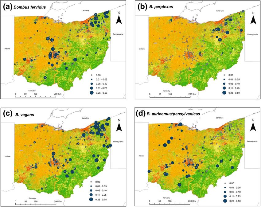
Fig. 5 Distribution and relative abundance of bumble bee species of conservation interest with Ohio land
use. a Bombus fervidus, b B. perplexus, c B. vagans, d B. auricomus/pensylvanicus. Land use is shown for
the state of Ohio (red—developed areas, orange—crop, yellow—herbaceous, green—forest, gray—other;
see Methods text for further details on land cover classification). Blue circles represent field survey sites
where a species was found, and are sized according to its proportional abundance in field surveys. Gray cir-
cles denote sites where a species was not present. The three dominant species that were present at almost all
sites are not included here, but see Electronic Supplementary Material (Fig. S1)
not predicted by the amount of forest in the landscape. Occurrence of only one species
was significantly predicted by habitat type (planted roadside for B. auricomus). The three
most common species, Bombus impatiens, B. griseocollis, and B. bimaculatus, were widely
distributed and did not show strong geographic patterns in occurrence (see Electronic Sup-
plementary Material Fig. S1 for distribution maps).
Discussion
We found substantial variation in distribution and abundance of 10 species of bumble bee
across the state of Ohio. This survey of over 23,000 bees at > 200 sites is among the larg-
est state or regional surveys yet reported, and provides a detailed and informative view
of Bombus diversity and abundance overall, and at the species level. Abundance of bum-
ble bees responded most strongly with habitat type, though landscape and geographic fac-
tors also explained some of the variance. However, these responses varied among species,
suggesting ways of tailoring conservation efforts to target taxa of interest. Abundance and
diversity were higher overall in planted habitats, including urban and roadside areas, than
13880 Biodiversity and Conservation (2021) 30:865–887 in unplanted habitats. These findings suggest that management efforts to provide forage for bumble bees are both successful and important. However, our results also confirm that some species of bumble bees respond to latitude and the broader landscape setting, espe- cially the amount of forest within 2 km. We know that forest is an important nesting habitat for many of the Midwestern bumble bee species (Lanterman et al. 2019), therefore inclu- sion of forested habitat in conservation plans is needed to promote nesting of these species and more diverse bumble bee communities in general. Careful siting of flower restorations to provide access to suitable nesting habitat may magnify the value of conservation efforts. Bumble bee abundance varied strongly among habitat types. However, those effects often depended on other variables, such as latitude and landscape-level forest cover. This makes sense for bumble bees because they have a long colony cycle and foraging ranges that are large enough to exceed habitat boundaries (Osborne et al. 1999; Woodgate et al. 2016). Colony success likely depends on access to multiple habitats at different times over the growing season. The positive relationship between total bumble bee abundance and cover of developed land in our study, as well as the high abundance of bumble bees in urban patches, concurs with others’ findings that at least some species thrive in human- dominated ecosystems (McFrederick and LeBuhn 2006; Ahrné et al. 2009; Reeher et al. 2020). Management of urban plantings for aesthetically pleasing blooms may result in more diverse, consistent, and concentrated flower resources that promote colony success compared to agricultural and natural non-urban landscapes (Goulson et al. 2002; Samuel- son et al. 2018). Planted habitats had higher abundance and diversity of Bombus, suggesting that man- agement efforts to promote pollinators are having positive effects. Restored meadows hosted abundant and diverse bumble bee communities commensurate with their profusion of attractive, rewarding wildflowers. Although usually smaller in size, urban patches of wildflowers had similar numbers of bumble bees as restored meadows. Planted hayfields, which were typically monocultures of red clover (Trifolium pratense) or alfalfa (Medicago sativa), yielded more than twice as many bumble bees as the average survey of unplanted natural early-successional fields or shrubby old fields. Planted hayfields, and to a lesser extent some roadsides, may have supported higher abundance because they exhibited sus- tained blooms of weedy flowers that are known bumble bee food plants (especially plants in the family Fabaceae, like Trifolium spp., Melilotus spp., Vicia spp., and Lathyrus spp.). Changes in management and decreasing abundance of hayfields in other areas of the north- ern USA have been associated with declines in occurrence and range of B. pensylvanicus, as well as B. fervidus (Richardson et al. 2019; Wood et al 2019). Likewise, flower restora- tions near agricultural areas that complement them in bloom times promoted bumble bee abundance, diversity, and colony success (Carvell et al. 2007, 2011; Williams et al. 2015; Wood et al. 2015). Sites that are dominated by weedy herbaceous vegetation and are mowed one to several times per season, such as hayfields and roadsides, provide repeated pulses of high-density forage (Carvell et al. 2006). However, the high level of disturbance may also destroy shel- tered nest sites and overwintering locations and thereby reduce their capacity to support nests of most species. Therefore, although we found that they attract large numbers of for- agers of many species, these habitats may be unsuitable for supporting long-term popula- tion growth unless the surrounding landscape offers nesting and overwintering opportuni- ties. Indeed, we found that the raw diversity of bumble bees along unplanted and planted roadsides increased with increased forest cover in the surrounding landscape (Electronic Supplementary Materials, Table S3). Forest positively affected species that nest in or near forest in our study, but not a species of conservation interest that nests in open grasslands, 13
Biodiversity and Conservation (2021) 30:865–887                                            881

B. pensylvanicus (Fig. 4). Promoting populations of grassland-nesting species may
require appropriate timing of mowing, in addition to protection or provisioning of nesting
resources. The question of whether habitats with abundant foragers but few nesting oppor-
tunities are ecological sinks is beyond the scope of this study, but deserves research focus.
   Bumble bee abundance in our surveys, but not diversity, increased over the season, most
likely reflecting growth in colony size. The addition of later emerging species, such as B.
griseocollis, B fervidus, B. pensylvanicus and B. auricomus (Colla and Dumesh 2010)
also contributed to the increase in abundance and especially to the diversity of bumble
bee communities through June. In August several species appeared to have completed their
colony cycle, so species diversity declined. This resulted in communities dominated by B.
impatiens, which is currently known to continue its colony cycle into the fall (Colla and
Dumesh 2010). In the past, the reduction in species richness may not have been as noticea-
ble, since B. affinis (now apparently absent from the state) and other declining species (e.g.,
B. vagans and B. fervidus) were once abundant late into the fall (Macior 1969; Colla and
Dumesh 2010). When monitoring for the presence of rare species, surveying the tail ends
of the season in spring and fall remains essential. However, our late-season surveys did not
offer useful insights into the habitat and geographic patterns of all species. By recognizing
seasonal changes and limiting analyses to the times of peak diversity when most species
were well-represented we were better able to evaluate the overall responses of bumble bee
communities to the environment.

Species specific patterns

The predominance of Bombus impatiens was consistent across all habitats and increased
over the season. Other studies of bumble bee communities in eastern North America have
found similar dominance of B. impatiens and suggest that this species is increasing in rela-
tive abundance compared to other species (Colla and Packer 2008; Cameron et al. 2011;
Jacobson et al. 2018; Richardson et al. 2019). No clear explanation for the success of B.
impatiens has surfaced, though our results suggest that its highly general habitat use and
long season of activity help it maintain large populations in many landscape contexts. In
turn, large populations likely buffer this species from loss of genetic diversity and demo-
graphic stochasticity that can lead to population decline (Herrmann et al. 2007; Dreier
et al. 2014). High diversity in worker size within B. impatiens nests may also allow colo-
nies to respond more efficiently than some other species to environmental changes (Austin
and Dunlap 2019), like fluctuations in food availability. Bombus griseocollis and B. bimac-
ulatus were also consistently present and abundant across our surveys. All three of these
potential competitors were abundant in the same habitats, raising the question of what sub-
tle differences in their biology allow them to coexist. Our findings demonstrate that these
three common Bombus species respond differently to habitat management and landscape.
Bombus impatiens showed fewer distinct responses than the other two species (Fig. 2),
seeming to flourish in almost all habitats. In contrast, Bombus griseocollis responded posi-
tively to forested landscapes in planted meadow or shrubby habitats, and showed GDD-
specific increases in planted meadow habitats (perhaps where its favored milkweed food
plants (Villalona et al. 2020) were abundant). Bombus bimaculatus responded differently,
with an increase at high latitudes, varied responses to GDD-habitat combinations, and an
earlier peak in abundance. Although there are certainly broad similarities in these three
dominant species, recognizing their differences will be necessary for effective conservation
of bumble bee communities. When generalizing about the response of a taxonomic group

                                                                                   13
882 Biodiversity and Conservation (2021) 30:865–887
to habitat quality, teasing apart species-specific effects helps to avoid attributing to all spe-
cies patterns that are driven primarily by the dominant species. Analysis of species-specific
foraging preferences may reveal further differences in their niches.
Several species of bumble bee that were found frequently in our survey of Ohio are
thought to be declining or rare in other areas. Two of these, B. vagans and B. fervidus were
each found in > 37% of our surveys (for reports of decline elsewhere see Grixti et al. 2009;
Williams et al. 2009; Colla and Packer 2008; Colla et al. 2012; Bartomeus et al. 2013;
Bushmann and Drummond 2015; Jacobson et al. 2018). On the other hand, our results
agree with those of others that B. perplexus is relatively uncommon (Colla and Packer
2008; Williams et al. 2009), found in only 21% of surveys. Due to the lack of rigorous
historical datasets on bee abundance and diversity in Ohio, we were not able to investigate
temporal trends in abundance as has been done in other recent literature (Colla and Packer
2008; Grixti et al. 2009; Cameron et al. 2011; Colla et al. 2012; Jacobson et al. 2018; Rich-
ardson et al. 2019; Wood et al. 2019). Though the stability of various species’ populations
is outside of the scope of this paper our results provide species-specific abundance and
distribution data that could be useful for future population stability analyses. In places that
lack historical data for comparison, such as Ohio, what we can do is focus on how current
bee distributions reflect current environments and use these data to inform conservation
strategies.
Although our survey was extensive, we did not have enough observations of the rarer
species to evaluate confidently possible influences on their abundance. This result is sober-
ing considering the scope of our study; we had > 450 h of observation over two years,
which provided > 23,000 bumble bee sightings, a level of sampling that is expensive and
uncommon. It is not clear whether rarity of these species is consistent with historical
patterns, reflects recent declines in their abundance, or is especially apparent because of
increased abundances of the three most common species. Nonetheless, we were able to
detect marked patterns regarding occurrence (presence/absence) and biogeography of the
rarer bumble bees. Bombus perplexus, which favored forested landscapes and the north-
ern part of the state, was associated with urban wildflower plantings. Bombus vagans and
B. fervidus were also more common in forested landscapes and at northern latitudes, but
not associated with urban patches. A species of conservation concern, B. pensylvanicus
(MacPhail et al. 2020; Richardson et al. 2019), that is affiliated with grasslands in our and
other studies (Colla and Dumesh 2010; Williams et al. 2014), was more frequently found
in the southern part of the state. Therefore, conserving or enhancing grassland habitat with
flowering forbs may be enough in the southern part of the state to support diversity, but in
the north habitat improvements near forests may be particularly effective.
One of the motivations for this survey was a desire to document the current distribution
and abundance of rare species, especially Bombus affinis and B. terricola. The former spe-
cies was once common in Ohio and was recently listed as federally endangered in the USA,
as a result of precipitous declines after about the year 1999 (Colla and Packer 2008; Grixti
et al. 2009; Williams et al. 2009; Cameron et al. 2011; Colla et al. 2012; Jacobson et al.
2018). Our results do not provide evidence that either of these species is now surviving
in Ohio. However, B. affinis has been observed in low abundance in the past several years
in the nearby states of Iowa, Illinois, Minnesota, and Wisconsin and in isolated mountain
meadows in Virginia and West Virginia (S. Droege, personal communication; P. Reeher,
personal observations in Virginia). Therefore, further monitoring may yet reveal its contin-
ued presence or recolonization in Ohio.
13Biodiversity and Conservation (2021) 30:865–887 883
Conclusions
Intensive sampling generates detailed datasets that can be used to improve monitoring
and habitat enhancements. In Ohio, the three most common species are nearly ubiquitous,
while distributions of three less common species vary with latitude and forest cover. More
observations of the rarer species are needed to understand how environmental factors influ-
ence their abundances here and across the region. Our finding that some species reach their
highest abundance in non-roadside habitats cautions that monitoring focused entirely along
roadsides could underestimate the abundance and distribution of some species of interest.
Our results provide a strong starting point for future bumble bee monitoring and for con-
servation intervention that targets less common species. While many surveys are or will be
funded and motivated by state-level conservation needs, important patterns in bumble bee
diversity and abundance need to also be considered at a broader geographic scale. There is
a strong need for collaboration among those conducting state-wide surveys to synthesize
regional and national data sets to address broad scale questions.
Supplementary Information The online version of this article (https://doi.org/10.1007/s10531-021-02121
-x) contains supplementary material, which is available to authorized users.
Acknowledgements This study was funded by the Ohio Department of Transportation (ODOT) grant num-
ber 30571. We thank Matt Perlik, Adrienne Earley, Megan Michael, and Phoenix Golnick Neal at ODOT for
initiating the project and providing guidance throughout. We appreciate the cooperation of Ohio State Parks
and Nature Preserves, Cuyahoga Valley National Park, Wayne National Forest, many county and municipal
parks districts, and many private landowners who provided access to study sites. We are grateful to the fol-
lowing student workers who assisted with field work: Audrey Bezilla, Sam Blechman, Jules Christensen,
Kevin Conroy, Christa Curtiss, Elizabeth DiCesare, John Ertle, Derek Foster, Amber Fredenburg, Samantha
Hodgson, Marko Jesenko, Kelly Peterson, and Brad Small. We also thank Denise Ellsworth of Ohio State
University Extension for help in publicizing the project and recruiting private land owners to participate.
John Ballas provided comments on earlier drafts of this manuscript.
Author contributions The Ohio Department of Transportation initiated this research. KG, RJM, JN, PR,
AL, and MV designed the study. All authors collected the data. JN, RJM, and KG analyzed the data, and
wrote the first draft of the manuscript. All authors helped revise the manuscript and approved the final draft.
Funding This study was funded by the Ohio Department of Transportation.
Data availability Our dataset from this study is publicly available on the online scientific data repository
Open Science Framework at https://osf.io/ygd9m/.
Compliance with ethical standards
Conflict of interest The authors have no conflicts of interest.
Ethical approval This manuscript is the authors’ own original research and has not been submitted or pub-
lished elsewhere simultaneously.
Informed consent All authors consent to the submission of this manuscript to the J Insect Conserv. All
authors consent to the publication of this manuscript if accepted in Biodiversity and Conservation.
Open Access This article is licensed under a Creative Commons Attribution 4.0 International License,
which permits use, sharing, adaptation, distribution and reproduction in any medium or format, as long
as you give appropriate credit to the original author(s) and the source, provide a link to the Creative Com-
mons licence, and indicate if changes were made. The images or other third party material in this article
are included in the article’s Creative Commons licence, unless indicated otherwise in a credit line to the
material. If material is not included in the article’s Creative Commons licence and your intended use is not
13You can also read