CAMELS-AUS: hydrometeorological time series and landscape attributes for 222 catchments in Australia
←
→
Page content transcription
If your browser does not render page correctly, please read the page content below

Earth Syst. Sci. Data, 13, 3847–3867, 2021
https://doi.org/10.5194/essd-13-3847-2021
© Author(s) 2021. This work is distributed under
the Creative Commons Attribution 4.0 License.

            CAMELS-AUS: hydrometeorological time series and
            landscape attributes for 222 catchments in Australia
               Keirnan J. A. Fowler1 , Suwash Chandra Acharya1 , Nans Addor2 , Chihchung Chou1,a , and
                                                  Murray C. Peel1
              1 Department  of Infrastructure Engineering, University of Melbourne, Parkville, Victoria, Australia
                                  2 Department of Geography, University of Exeter, Exeter, UK
                 a now at: Department of Earth Sciences, Barcelona Supercomputing Centre, Barcelona, Spain

                             Correspondence: Keirnan J. A. Fowler (fowler.k@unimelb.edu.au)

                                  Received: 2 September 2020 – Discussion started: 4 January 2021
                             Revised: 28 May 2021 – Accepted: 18 June 2021 – Published: 6 August 2021

       Abstract. This paper presents the Australian edition of the Catchment Attributes and Meteorology for Large-
       sample Studies (CAMELS) series of datasets. CAMELS-AUS (Australia) comprises data for 222 unregulated
       catchments, combining hydrometeorological time series (streamflow and 18 climatic variables) with 134 at-
       tributes related to geology, soil, topography, land cover, anthropogenic influence and hydroclimatology. The
       CAMELS-AUS catchments have been monitored for decades (more than 85 % have streamflow records longer
       than 40 years) and are relatively free of large-scale changes, such as significant changes in land use. Rating curve
       uncertainty estimates are provided for most (75 %) of the catchments, and multiple atmospheric datasets are in-
       cluded, offering insights into forcing uncertainty. This dataset allows users globally to freely access catchment
       data drawn from Australia’s unique hydroclimatology, particularly notable for its large interannual variability.
       Combined with arid catchment data from the CAMELS datasets for the USA and Chile, CAMELS-AUS con-
       stitutes an unprecedented resource for the study of arid-zone hydrology. CAMELS-AUS is freely downloadable
       from https://doi.org/10.1594/PANGAEA.921850 (Fowler et al., 2020a).

1   Introduction                                                   nent of recent hydrological research (see review by Addor et
                                                                   al., 2019).
For some time, the ideals of “comparative hydrology” and              However, issues of data availability and commensurabil-
“large-sample hydrology” have been advanced as com-                ity, which are endemic to environmental sciences, are ex-
plementary and necessary components of hydrology (e.g.             acerbated for large-sample hydrology. Large samples may
Falkenmark and Chapman, 1989; Andréassian et al., 2006;            cross jurisdictions or data providers or require harmonisa-
Gupta et al., 2014). Alongside traditional hydrological stud-      tion across different data formats or nomenclatures (e.g.
ies, which may focus on a single catchment or possibly com-        hydrometric-data quality codes and flags) and are more likely
pare results among several catchments within a region, large-      to suffer from spatial gaps due to different data sharing poli-
sample studies aim to establish the generality of results and      cies of water agencies (Viglione et al., 2010; Addor et al.,
to test paradigms applicable on regional to global scales (e.g.    2019). Thus, the importance of FAIR data (findable, accessi-
McMahon et al., 1992; Peel et al., 2004; Kuentz et al., 2017;      ble, interoperable and reusable; see Wilkinson et al., 2016
Ghiggi et al., 2019; Mathevet et al., 2020). Large samples of      and the Open Data Charter, 2015) in hydrology is ampli-
catchments are also insightful for certain tasks, such as pre-     fied in large-sample hydrology, and there is a clear need for
diction in ungauged basins (e.g. Pool et al., 2019; Kratzert       open publication of datasets wherever possible to allow equal
et al., 2019b) or training and evaluation of machine learning      access. Such policies also encourage hydrologists to work
algorithms (e.g. Kratzert et al., 2018; Shen, 2018; Kratzert et    across boundaries – an important ideal since the spatial dis-
al., 2019a). Thus, large-sample studies are a growing compo-

Published by Copernicus Publications.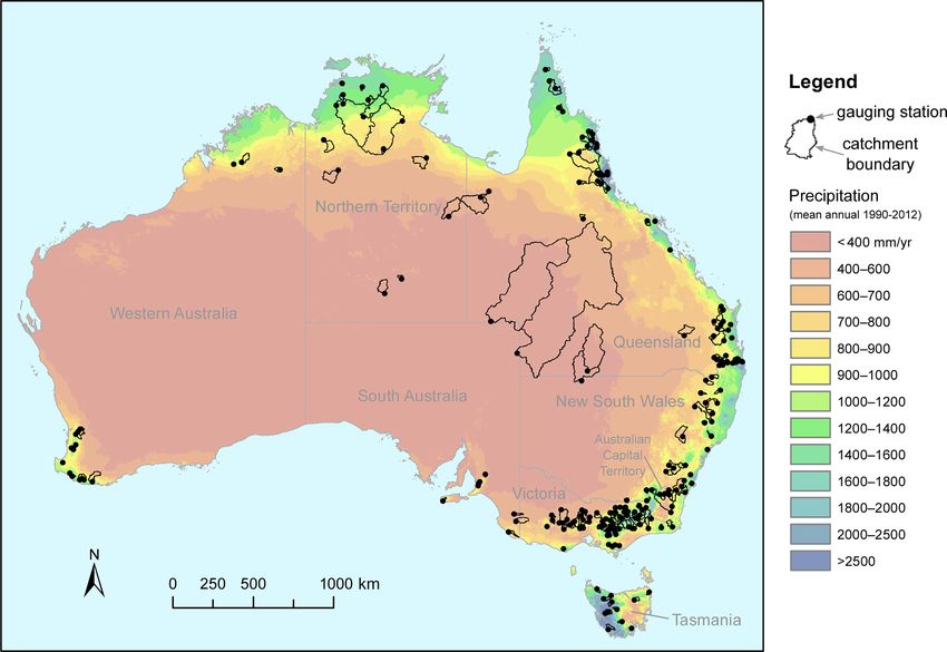
3848                           K. J. A. Fowler et al.: Hydrometeorological time series and landscape attributes for Australia

tribution of hydrologists globally reflects neither the spread     2     Rationale
of interesting hydrological environs nor the pressing need for
hydrological insights to inform policy.                            This section lays out the motivations underpinning the re-
   Responding to these needs, multiple recent projects have        lease of this dataset for Australia. It also outlines why
publicly released large-sample hydrological datasets (e.g.         CAMELS-AUS takes its present form, including two chief
Arsenault et al., 2016; Do et al., 2018; Lin et al., 2019;         aspects: catchment selection and inclusion of local versus
Linke et al., 2019; Olarinoye et al., 2020). Here we contribute    global datasets.
to one such ongoing project – the Catchment Attributes
and Meteorology for Large-sample Studies, or CAMELS,               2.1    Motivation: Australian hydroclimate and its place in
project. Originally launched for the United States (Newman                the study of arid-zone hydrology and hydrology
et al., 2015; Addor et al., 2017), CAMELS datasets now ex-                under climatic change
ist for Chile (Alvarez Garreton et al., 2018), Great Britain
(Coxon et al., 2020) and Brazil (Chagas et al., 2020). The         Every region on earth is unique and has characteristics of
defining features of a CAMELS dataset are that they com-           interest for hydrological study. Within Australia and for
plement data on streamflow (which are often publicly avail-        CAMELS-AUS, three characteristics are noted here. Firstly,
able) with other data types: (i) pre-processed climatic data       Australia contains many arid landscapes, and considerable
for each catchment, such as would be required to run a hy-         advances in arid-zone hydrology have been made there (e.g.
drological model, and (ii) catchment attributes which charac-      Western et al., 2020). CAMELS-AUS contains more than 20
terise various aspects of the catchment without the need for       arid-zone rivers (depending on definition, but see Fig. 1), so
field visitation (impractical for large samples). They also sup-   the publication of the dataset opens the study of these rivers
port download of the entire dataset in contrast to agency web-     to a global pool of scientists. Added together with included
sites, which may only support one-at-a-time download (if at        arid-zone rivers in the USA and Chile (Addor et al., 2017;
all). Lastly, whereas government agencies reserve the right        Alvarez-Garreton et al., 2018), the CAMELS datasets to-
to retrospectively re-process their streamflow data (e.g. due      gether provide a significant sample for the study of arid-zone
to rating curve changes), CAMELS datasets enable repeata-          hydrology.
bility because a given CAMELS release effectively “freezes”           Secondly, Australian catchments tend to have lower
the data, creating a consistent version that is available indef-   rainfall-to-runoff ratios, linked to higher evaporative de-
initely via a persistent digital object identifier (DOI).          mand. As shown in Fig. 2d, the median rainfall–runoff ratio
   The present dataset focusses on the continent of Australia,     among Australian catchments is approximately 0.25, com-
including the southern state of Tasmania but excluding other       pared to approximately 0.4 for the rest of the world. Aus-
Australian territories. Australia is the world’s sixth-largest     tralian catchments are often water-limited (at least on a
country (approximately 7.7 × 10⁶ km2 ) and is comparable in        seasonal basis), providing different modelling challenges to
size to the conterminous USA or Europe, but the hydrologi-         energy-limited catchments from higher latitudes.
cally active parts of the country tend to be limited to coastal       Finally, a notable characteristic of Australian hydrocli-
regions, with the interior being semi-arid or arid (Fig. 1; see    matology is its tendency for multi-year spells of climatic
also Knoben et al., 2018). Thus, dense gauging of stream-          anomalies of larger magnitude compared to most other re-
flow covers only a small proportion of the total area, with        gions of the world (Peel et al., 2005), due partly to the
the remaining areas providing few gauged locations. While          strong influence of climate teleconnections such as the El
sparsely gauged, the dry parts of Australia provide interest-      Niño–Southern Oscillation (ENSO; e.g. Peel et al., 2002;
ing arid-zone catchment examples, many of which are in-            Verdon-Kidd and Kiem, 2009). Recent severe droughts have
cluded in the CAMELS-AUS, the Australian edition, dataset.         affected south-eastern Australia, including the 13-year Mil-
In addition to arid regions, Australia includes northern areas     lennium Drought (Van Dijk et al., 2014), which provided
with tropical climate and southern areas with temperate cli-       the opportunity for knowledge sharing with other drought-
mate.                                                              prone regions (Aghakouchak et al., 2014) and supplied many
   This paper is structured as follows. In Sect. 2 we describe     case studies of hydrological model failure (i.e. the high bias
the rationale for the dataset, including considerations of why     and low model performance in differential split sample test-
Australian hydroclimate is interesting and relevant to hydrol-     ing reported by e.g. Saft et al., 2016), which are under on-
ogists globally; and factors shaping the dataset, including lo-    going investigation (e.g. Fowler et al., 2020b). In the con-
cal data availability. Section 3 provides a technical descrip-     text of providing credible runoff projections, case studies
tion of the dataset and forms the bulk of the paper. Sections 4    of long droughts are the only means by which hydrologists
and 5 explain CAMELS-AUS data availability and conclude            can test hypotheses regarding how catchments respond phys-
the paper, respectively.                                           ically to the onset of drier conditions, including aspects of
                                                                   long “memory” (e.g. Fowler et al., 2020b) and potential to
                                                                   shift behaviour, possibly in a quasi-permanent fashion (e.g.
                                                                   Peterson et al., 2021). Thus, it is hoped that the public re-

Earth Syst. Sci. Data, 13, 3847–3867, 2021                                           https://doi.org/10.5194/essd-13-3847-2021
K. J. A. Fowler et al.: Hydrometeorological time series and landscape attributes for Australia                               3849

Figure 1. Location of the 222 CAMELS-AUS flow gauging stations and catchments, along with mean annual precipitation (from Jones et
al., 2009) and Australian states and territories.

lease of datasets such as CAMELS-AUS may hasten scien-              project selected a large set of gauging stations, each on un-
tific progress towards more defensible and robust hydrologi-        regulated streams, to serve as a “platform to investigate long-
cal models.                                                         term trends in water resource availability” (Turner et al.,
                                                                    2012, p. 1555). The project has a website for provision of
2.2   Context: hydrometeorological monitoring in Australia          streamflow data to the public (http://www.bom.gov.au/water/
                                                                    hrs/, last access: 29 July 2021).
Systematic climatic measurement in Australia extends back              We adopted the Hydrologic Reference Stations as the basis
to the late 1800s (e.g. Ashcroft et al., 2014), with widespread     for CAMELS-AUS for three reasons:
streamflow gauging of headwater catchments commencing
from the 1950s and ’60s. Meteorological monitoring is the             – The selection criteria used by the BOM, including
responsibility of a federal Bureau of Meteorology (BOM),                record length, lack of regulation and stationarity of
but streamflow monitoring falls to the states and territories           anthropogenic influence (see Sect. 3.2), are consistent
of Australia rather than the federal government (Skinner and            with the aim of the CAMELS project to provide high-
Langford, 2013). Thus, Australian streamflow data have his-             quality scientific data.
torically been dispersed between its six states and two terri-
tories (Fig. 1), and while quality control is relatively well es-     – Considerable effort has already been expended by the
tablished, methods and formats (e.g. quality codes and flags)           BOM to standardise and quality-check the streamflow
are not consistent between states and territories. Since the            data, which was only possible via contacts with state
2000s this situation has partially been rectified after federal         agencies that are not necessarily available to academic
legislation required the BOM to collate data from the states            authors (for an example, see BOM, 2020). It is logical
under new “water information” powers (Vertessy, 2013).                  to take advantage of this prior effort.

                                                                      – The Hydrologic Reference Stations have attained a de-
2.3   Catchment choice: the Hydrologic Reference
                                                                        gree of acceptance within the Australian hydrological
      Stations dataset
                                                                        community, partly due to extensive consultation with
Under its new responsibilities the BOM initiated several na-            stakeholders during development (see Sect. 3.2). Also,
tional hydrological projects, one of which is called the Hy-            they have been adopted by numerous academic stud-
drologic Reference Stations project (Turner et al., 2012). This         ies (e.g. Zhang et al., 2014, 2016; Wright et al., 2018;

https://doi.org/10.5194/essd-13-3847-2021                                          Earth Syst. Sci. Data, 13, 3847–3867, 2021
3850                              K. J. A. Fowler et al.: Hydrometeorological time series and landscape attributes for Australia

                                                                        one hand, global datasets are important to facilitate intercon-
                                                                        tinental comparisons. On the other hand, when local datasets
                                                                        are available, they are generally the highest-quality informa-
                                                                        tion that exists for a given region (e.g. Acharya et al., 2019).
                                                                        With the advent of large-sample hydrology, it is now possi-
                                                                        ble to conduct near-global studies using very large samples
                                                                        of catchments (e.g. over 2000 in Mathevet et al., 2020), and
                                                                        future studies might compose such large samples by com-
                                                                        bining continental-scale datasets like the various CAMELS.
                                                                        However, the lack of standardised approaches and sources
                                                                        between national large-sample datasets remains a key limita-
                                                                        tion of large-sample studies (Addor et al., 2019).
                                                                           The approach followed by the CAMELS datasets so far is
                                                                        to use the best possible data available for each country, so
                                                                        national datasets have been prioritised over global datasets.
                                                                        In some cases, global datasets have been employed, for in-
                                                                        stance the Global Lithological Map (Hartmann and Moos-
                                                                        dorf, 2012) in CAMELS datasets for the USA and Chile
                                                                        or the Multi-Source Weighted-Ensemble Precipitation (Beck
                                                                        et al., 2017) in CAMELS-CL. But overall, the best national
                                                                        data products were selected for each country, leveraging the
Figure 2. Mean annual values of hydrological variables for the
global set of 699 catchments presented by Peel et al. (2010;
                                                                        knowledge of CAMELS creators. This enables global users,
nAustralia = 123, nrest of world = 576). Boxplots show the 5th, 25th,   who may not be familiar with these national products, to
50th, 75th and 95th percentiles. Potential evapotranspiration in this   benefit from this local knowledge. It also gives direct ac-
dataset is a reference crop estimate using a method similar to Harg-    cess to the best available data to users whose study focusses
reaves’ method, as outlined in Adam et al. (2006).                      on catchments from a single country (see e.g. intercompar-
                                                                        isons in Acharya et al., 2019). In keeping with this approach,
                                                                        the priority was given to national data products to produce
      McInerney et al., 2017; Fowler et al., 2016, 2018,                CAMELS-AUS.
      2020b).                                                              In parallel, efforts are ongoing to increase the consistency
                                                                        among the CAMELS datasets (in terms of data products used
It is noted that this choice is not intended to limit future in-        to derive the time series and catchment attributes and also
clusion of a wider range of stations and catchments. We en-             naming conventions and data format; see Addor et al., 2019)
visage that the Hydrologic Reference Stations may provide               in order to create a dataset that is globally consistent. This
the nucleus for future versions of the CAMELS-AUS dataset,              is part of a second phase, which will build upon the cur-
while the current selection provides a sensible and pragmatic           rent phase, which is focussed on the release of national prod-
starting point. The Hydrologic Reference Station dataset it-            ucts, such as CAMELS-AUS. To contribute to this effort, we
self may be subject to future expansion, which would inform             have supplied the CAMELS-AUS catchment boundaries and
future CAMELS-AUS versions. Furthermore, whereas the                    gauge locations. Because of these ongoing efforts, our ex-
Hydrologic Reference Stations project, by definition, sought            pectation is that the data introduced here, derived from Aus-
catchments which are minimally disturbed (or at least hav-              tralian sources, will in time be complemented by data derived
ing stationarity of anthropogenic influence), future versions           from global datasets.
could be more inclusive so as to cater for studies examin-
ing diverse anthropogenic influences including changes over
time – an approach already taken by CAMELS-GB (Great
Britain; Coxon et al., 2020) and CAMELS-BR (Brazil; Cha-                3   CAMELS-AUS dataset technical description
gas et al., 2020). In summary, the current form of CAMELS-
AUS should not be interpreted as setting a norm for future              The previous section outlined key decisions made for
versions (or other datasets).                                           CAMELS-AUS; i.e. it is based on the Hydrologic Refer-
                                                                        ence Stations, and its data are derived from Australian rather
2.4    Local versus global datasets                                     than global sources. This section provides more detail and
                                                                        presents each aspect of the dataset in turn. Work not under-
A key choice in developing CAMELS-AUS was whether to                    taken by the present authors (e.g. earlier efforts by the BOM
use local or global datasets (or both) when extracting hy-              for the Hydrologic Reference Stations project) is clearly
drometeorology time series and catchment attributes. On the             marked. In many cases, sub-sections end with an “Included

Earth Syst. Sci. Data, 13, 3847–3867, 2021                                              https://doi.org/10.5194/essd-13-3847-2021
K. J. A. Fowler et al.: Hydrometeorological time series and landscape attributes for Australia 3851
in dataset” section to clearly outline items in the online Included in dataset. The following variables are provided
repository related to the sub-section text. in the CAMELS-AUS attribute table (see Table 1): station
Before presenting the details, we note that the online ID, station name (including river name and station name),
repository of the dataset (Fowler et al., 2020a) includes the drainage division and river region (out of 13 drainage divi-
following: sions and 218 river regions across Australia). Unfortunately,
information is not available about which catchments were in-
– a file containing the overall attribute table containing all cluded or excluded under the above rules.
non-time-series data (see Tables 1, 3 and 4);
– 27 time series files, each containing data for all catch- 3.2 Catchment boundaries
ments for a given hydroclimatic variable (see Table 2); For all but 10 of the catchments, catchment boundaries were
and derived via flow path analysis (using Esri’s Arc Hydro)
– extra files such as shapefiles and readme files as noted of topographic data undertaken by the authors. The input
below. data were (i) the post-processed and hydrologically enforced
DEM of Gallant et al. (2012), which is derived from the 1 s
(approximately 30 m) grid Shuttle Radar Topography Mis-
3.1 Catchment selection rules sion (SRTM) dataset, and (ii) the location of the streamflow
gauges as provided by the BOM. The Arc Hydro analysis
Given the decision (Sect. 2.2 above) to base the CAMELS- determines the apparent position of streams from the DEM
AUS dataset on the BOM’s Hydrologic Reference Stations, data, and it was found that the published locations rarely
this sub-section summarises the process of catchment selec- fall precisely on these digital streamlines. The mismatch is
tion undertaken earlier by the BOM, as described in Turner unsurprising given that location data may be decades old,
et al. (2012). and significant figures may have been truncated with the pas-
sage of data between databases (or never reported in the first
– Initial selection: 246 potential stations were initially se-
place). Also, the position of the digital streamline may or
lected based on the three criteria of (i) record length
may not match reality, particularly in flat landscapes. To de-
(minimum of 1975 onwards), (ii) availability of data in-
rive catchment areas, the BOM-published gauge locations
cluding historic rating curve information and (iii) lack
were shifted to the nearest streamline with expected catch-
of regulation by large dams.
ment area. This movement was generally less than 200 m.
– Invitation for stakeholders to suggest additional sta- As noted, this method was used for most catchments, with
tions: BOM consulted with 70 stakeholders from fed- the following exceptions:
eral, state and territory agencies and water authorities, – For the six largest catchments (A0030501, A0020101,
who were given the opportunity to add new stations to G8140040, G9030250, 424002 and 424201A), this pro-
the list. This enlarged the list to 362 stations. cess was not undertaken due to excessive computational
requirements. For context, the largest catchment is ap-
– Targeted fact-finding: to elicit information about each
proximately the size of the United Kingdom (see Fig. 1).
candidate station and catchment, the relevant agencies
were asked a series of questions about the catchments in – For a further four catchments (A2390519, A2390523,
their jurisdiction relating to both past and present prac- 307473 and 606185), the Arc Hydro process resulted
tices. Topics included diversions, irrigation structures, in a catchment boundary that was inconsistent with the
upstream point source discharge, land clearing, forestry, boundaries displayed on the Hydrologic Reference Sta-
urbanisation, fire and farm dams. tion website. Although degraded for fast mapping, the
website boundaries show the approximate position of
– Final selection: the final selection process considered all the boundary as agreed with stakeholders and agencies
the above information. A good coverage of Australia’s who have local knowledge. Therefore, in cases of obvi-
various hydroclimatic regions was desired, although this ous mismatch, the Arc Hydro-derived boundaries were
is inherently limited by the coverage of the gauging net- assumed to be in error. Despite the “blockiness” of the
work. Where possible, only stations with < 5 % missing website boundaries, they were considered to be a better
data and3852 K. J. A. Fowler et al.: Hydrometeorological time series and landscape attributes for Australia
Table 1. Basic catchment information provided in the attribute table of CAMELS-AUS.
Short name Description Data source and notes
station_id Station ID used by the Australian Water Resources Council Hydrologic Reference Stations (HRS)
project, Bureau of Meteorology (BOM)
station_name River name and station name
http://www.bom.gov.au/water/hrs (last
drainage_division Drainage division of the 13 defined by the BOM access: 29 July 2021)
river_region River region of the 218 defined by the BOM
notes General notes about data issues and/or catchment area calculations
lat_outlet Latitude and longitude at outlet. Note that in most cases this will be
slightly different to the BOM-published value because most outlets
long_outlet
needed to be moved onto a digital streamline in order to facilitate
flow path analysis.
lat_centroid Latitude and longitude at centroid of the catchment
This study;
long_centroid
for daystart_Q, see Jian et al. (2017)
map_zone Map zone used to calculate catchment area (function of longitude)
catchment_area Area of upstream catchment in square kilometres
state_outlet Indicates which state or territory of Australia the outlet is within
state-alt If the catchment crosses a state or territory boundary, the alterna-
tive state or territory is listed here; otherwise “n/a”, meaning not
applicable.
daystart Time (UTC) for midnight local standard time (for state_ outlet).
This is the day start time for Tmax and Tmin (see Sect. 3.5.2).
daystart_P Time (UTC) for 09:00 local standard time (for state_ outlet); 09:00
is when once-per-day precipitation measurements are reported (see
Sect. 3.5.2).
daystart_Q Time (UTC) for streamflow day start time, assuming local standard
time for state_outlet. This varies by state or territory (Sect. 3.5.2).
nested_status “Not nested” indicates the catchment is not contained within any
other. “Level1” means it is contained within another, except in cases
where it is contained in another “Level1” catchment, in which case
it is marked “Level2”. There are no “Level3” catchments in the
present dataset.
next_station_ds For “Level1” and “Level2” nested catchments, NextStationDS
(“DS” meaning downstream) indicates the catchment they are con-
tained within.
num_nested_within Indicates how many catchments are nested within this catchment
start_date Streamflow gauging start date (yyyymmdd)
HRS (see above)
end_date Streamflow gauging end date (yyyymmdd)
prop_missing_data Proportion of data missing between start date and end date
Included in dataset. The main inclusions are a point shape- ures. As listed in Table 1, the CAMELS-AUS attribute ta-
file of adopted gauge locations and a polygon shapefile of ble lists the coordinates of the catchment outlet and centroid,
adopted catchment areas. Further information included are along with notes which expand on issues listed above, on a
a point shapefile of BOM-published gauge locations, poly- catchment-by-catchment basis.
gon shapefile of website-mapped boundaries, and readme file
explaining the above logic but in more detail and with fig-
Earth Syst. Sci. Data, 13, 3847–3867, 2021 https://doi.org/10.5194/essd-13-3847-2021K. J. A. Fowler et al.: Hydrometeorological time series and landscape attributes for Australia 3853
Table 2. Hydrometeorological time series data supplied with CAMELS-AUS. All time steps are daily. All non-streamflow data were pro-
cessed as part of the CAMELS-AUS project to extract catchment averages from Australia-wide Australian Water Availability Project (AWAP)
and Scientific Information for Land Owners (SILO) grids.
Category File name Source data Description and comments Unit
Streamflow streamflow_MLd.csv Streamflow (not gap-filled) ML d−1
Hydrologic Reference Stations (HRS) project, Bureau
streamflow_MLd_infilled.csv of Meteorology (BOM) http://www.bom.gov.au/water/ Streamflow gap-filled by the BOM us- ML d−1
hrs (last access: 29 July 2021) ing GR4J (Perrin et al., 2003)
streamflow_mmd.csv Streamflow (not gap-filled) expressed mm d−1
as depths relative to CAMELS-AUS-
adopted catchment areas (Table 1)
streamflow_QualityCodes.csv Quality codes and flags as supplied –
by the HRS website, with meanings
listed at http://www.bom.gov.au/
water/hrs/qc_doc.shtml (last access:
30 July 2021)
Precipitation precipitation_awap.csv BOM’s Australian Water Availability Project (AWAP), Catchment average precipitation mm d−1
(Jones et al., 2009; http://www.bom.gov.au/climate/
precipitation_var_awap.csv Spatial internal variance in precipitation mm2 d−2
maps/, last access: 30 July 2021); AWAP provides 0.05◦
as calculated by the “AWAPer” tool (Pe-
grids.
terson et al., 2020).
precipitation_silo.csv Catchment average precipitation
Actual and et_short_crop_silo.csv FAO56 short-crop PET (see FAO, 1998)
potential Scientific Information for Land Owners (SILO)
et_tall_crop_silo.csv ASCE tall-crop PET (see ASCE, 2000)
evapo- project, Government of Queensland (Jeffrey et al.,
traspiration et_morton_wet_silo.csv 2001; http://www.longpaddock.qld.gov.au, last access: Morton (1983) wet-environment areal
(AET and PET) 30 July 2021); SILO provides 0.05◦ grids. PET over land
et_morton_point_silo.csv Morton (1983) point PET mm d−1
et_morton_actual_silo.csv Morton (1983) areal AET
evap_morton_lake_silo.csv Morton (1983) shallow-lake evapora-
Evaporation tion
evap_pan_silo.csv Interpolated Class A pan evaporation
evap_syn_silo.csv Interpolated synthetic extended Class A
pan evaporation (Rayner, 2005)
tmax_awap.csv AWAP (see above)
Daily maximum temperature
Temperature tmax_silo.csv SILO (see above) ◦C
tmin_awap.csv AWAP (see above)
Daily minimum temperature
tmin_silo.csv SILO (see above)
solarrad_awap.csv AWAP (see above)
Solar radiation MJ m−2
radiation_silo.csv SILO (see above)
vprp_awap.csv AWAP (see above)
Other variables Vapour pressure hPa
vp_silo.csv
vp_deficit_silo.csv Vapour pressure deficit hPa
SILO (see above)
rh_tmax_silo.csv Relative humidity at the time of maxi- %
mum temperature
rh_tmin_silo.csv Relative humidity at the time of mini- %
mum temperature
mslp_silo.csv Mean sea level pressure hPa
3.3 Catchment area and nestedness was placed within a zone, and this zone was used to calcu-
late area using the standard tool within Esri’s ArcMap. In-
To calculate catchment areas, the catchment boundaries were spection of catchment boundaries revealed that some of the
first projected into the appropriate local coordinate system catchments are “nested” (i.e. entirely contained) within oth-
under the Map Grid of Australia (MGA). Due to Australia’s ers, for example, when two gauges lie on the same stream
size, the MGA defines different coordinate systems based (one downstream of the other) and both have been included
on longitude. Using the catchment centroid, each catchment
https://doi.org/10.5194/essd-13-3847-2021 Earth Syst. Sci. Data, 13, 3847–3867, 20213854 K. J. A. Fowler et al.: Hydrometeorological time series and landscape attributes for Australia
Table 3. Flow uncertainty information, climatic indices and streamflow signatures provided in the attribute table of CAMELS-AUS.
Short name Description Units Data source and notes
q_uncert_NumCurves Flow uncertainty: number of rating curves considered in –
analysis by McMahon and Peel (2019) and total number
q_uncert_N
(Q_uncert_N) of days the curves apply to
q_uncert_q10 Q10 (i.e. flow exceeded 90 % of the time) flow value with 95 % mm d−1
confidence limits. Note that this is only calculated considering McMahon and Peel (2019)
q_uncert_q10_upper %
days for which rating curves are available.
q_uncert_q10_lower %
q_uncert_q50 mm d−1
As above but for the median flow
q_uncert_q50_upper %
q_uncert_q50_lower %
q_uncert_q90 mm d−1
As above but for Q90 (flow exceeded 10 % of the time)
q_uncert_q90_upper %
q_uncert_q90_lower %
p_mean Mean daily precipitation mm d−1
Climatic signatures are calculated using
pet_mean Mean daily potential evapotranspiration (PET) (Morton’s wet mm d−1 code from Addor et al. (2017) using the
environment) following datasets (cf. Table 1):
– Precipitation is based on AWAP rainfall.
pet_mean
aridity Aridity p_mean – – PET is based on SILO Morton’s wet
environment PET.
p_seasonality Precipitation seasonality (0: uniform; +’ve: Dec/Jan peak; –
– Temperature data are based on AWAP
−’ve: Jun/Jul peak)
temperature.
frac_snow Fraction of precipitation on days colder than 0 ◦ C – For p_seasonality see Eq. (14) in
Woods (2009).
high_prec_freq Frequency of high-precipitation days, ≥ 5 times p_mean d yr−1
high_prec_dur Average duration of high-precipitation events Days
high_prec_timing Season during which most high-precipitation days occur (djf, Season
mam, jja, or son)
low_prec_freq Frequency of dry days (≤ 1 mm d−1 ) d yr−1
low_prec_dur Average duration of low-precipitation periods Days
(days ≤ 1 mm d−1 )
low_prec_timing Season during which most dry days occur (djf, mam, jja, or son) Season
q_mean Mean daily streamflow mm d−1
Hydrologic signatures are calculated using
runoff_ratio Ratio of mean daily streamflow to mean daily precipitation –
code from Addor et al. (2017). Where re-
stream_elas Sensitivity of annual streamflow to annual rainfall changes – quired, climate datasets are the same as
above.
slope_fdc Slope of flow duration curve (log transformed) from percentiles –
Original sources of signature formulations:
33 to 66
– stream_elas – Sankarasubramanian et
baseflow_index Baseflow as a proportion of total streamflow, calculated by re- – al. (2001);
cursive filter – slope_fdc – Sawicz et al. (2011);
– baseflow_index – Ladson et al. (2013);
hdf_mean Mean half-flow date (date marking the passage of half the year’s Day of year
and
flow), calculated according to April–March water years
– hdf_mean – Court (1962).
Q5 5 % flow quantile (low flow: flow exceeded 95 % of the time) mm d−1
Q95 95 % flow quantile (high flow: flow exceeded 5 % of the time) mm d−1
high_q_freq Frequency of high-flow days (≥ 9 times mean daily flow) d yr−1
high_q_dur Average duration of high-flow events Days
low_q_freq Frequency of low-flow days (K. J. A. Fowler et al.: Hydrometeorological time series and landscape attributes for Australia 3855
Table 4. Catchment attributes included in the attributes table of CAMELS-AUS (apart from climatic and hydrologic indices).
Short name Description Unit Data source Notes and references
geol_prim
Two most common geologies (see list in cell below) with corre-
geol_prim_prop –
sponding proportions
geol_sec
geol_sec_prop
Pre-processed by
Geoscience Australia (2008)
Geology and soils
unconsoldted Stein et al. (2011)
Proportion of catchment taken up by individual geological
types, specifically unconsolidated rocks, igneous rocks, silici-
igneous
clastic and undifferentiated sedimentary rocks, carbonate sed- –
silicsed imentary rocks, other sedimentary rocks, metamorphic rocks,
and mixed sedimentary and igneous rocks
carbnatesed
othersed
metamorph
sedvolc
oldrock Catchment proportion of old bedrock –
claya Per cent of clay in the soil A and B horizons for the stream
% National Land and Water Pre-processed by
valley in the reach containing gauging station
clayb Resources Audit (2001) Stein et al. (2011)
sanda As above, but per cent of sand in the soil A horizon %
solum_thickness Mean soil depth considering all principle profile forms m McKenzie et al. (2000) –
ksat Saturated hydraulic conductivity (areal mean) mm h−1 Pre-processed by
Western and McKenzie (2004)
Stein et al. (2011)
solpawhc Solum plant available water holding capacity (areal mean) mm
elev_min Elevation above sea level at gauging station m Gallant et al. (2009) –
elev_max Pre-processed by
Topography and geometry
Catchment maximum and mean elevation above sea level m Hutchinson et al. (2008)
Stein et al. (2011)
elev_mean
elev_range Range of elevation within catchment: elev_ max-elev_min m –
mean_slope_pct Mean slope, calculated on a grid-cell-by-grid-cell basis % Gallant et al. (2012) –
upsdist Maximum flow path length upstream km Pre-processed by Stein et
al. (2011);
strdensity Ratio: total length of streams / catchment area km−1
for strahler, see
Hutchinson et al. (2008)
strahler Strahler stream order at gauging station – Strahler (1957);
for elongratio, see Gordon et
elongratio Factor of elongation as defined in Gordon et al. (1992) – al. (1992)
relief Ratio: mean elevation above outlet / max elevation above outlet –
reliefratio Ratio: elevation range / flow path distance –
mrvbf_prop_0 Proportion of catchment occupied by classes of Multi- – CSIRO (2016) Gallant and Dowling (2003)
through to Resolution Valley Bottom Flatness (MRVBF). These indicate
mrvbf_ prop_ 9 areas subject to deposition. Broad interpretations are 0 – ero-
sional, 1 – small hillside deposit, 2–3 – narrow valley floor, 4
– valley floor, 5–6 – extensive valley floor, 7–8 – depositional
basin, 9 – extensive depositional basin.
confinement Proportion of stream segment cells and neighbouring cells that – Hutchinson et al. (2008) Pre-processed by
are not valley bottoms (as defined by MRVBF) Stein et al. (2011)
https://doi.org/10.5194/essd-13-3847-2021 Earth Syst. Sci. Data, 13, 3847–3867, 20213856 K. J. A. Fowler et al.: Hydrometeorological time series and landscape attributes for Australia
Table 4. Continued.
Short name Description Unit Data source Notes and references
lc01_extracti Proportion of catchment occupied by land cover categories
within the Dynamic Land Cover Dataset (DLCD):
lc 03_waterbo
Land cover and vegetation
mines and quarries (ISO name: extraction sites)
lc 04_saltlak lakes and dams (inland water bodies)
salt lakes (salt lakes)
lc 05_irrcrop
irrigated cropping (irrigated cropping)
lc06_irrpast irrigated pasture (irrigated pasture)
irrigated sugar (irrigated sugar)
lc07_irrsuga
rain-fed cropping (rainfed cropping)
Note that the source dataset has
lc08_rfcropp rain-fed pasture (rainfed pasture)
13 time slices; these attributes
rain-fed sugar (rainfed sugar)
lc09_rfpastu – Lymburner et al. (2015) indicate the temporal average.
wetlands (wetlands)
The time slices are separately
lc10_rfsugar closed tussock grassland (tussock grasses – closed)
supplied with CAMELS–AUS.
alpine meadows (alpine grasses – open)
lc11_wetlands open hummock grassland (hummock grasses – open)
lc14_tussclo open tussock grasslands (tussock grasses – open)
scattered shrubs and grasses (shrubs and grasses – sparse –
lc15_alpineg scattered)
lc16_openhum dense shrubland (shrubs – closed)
open shrubland (shrubs – open)
lc18_opentus closed forest (trees – closed)
lc19_shrbsca open forest (trees – open)
open woodland (trees – scattered)
lc24_shrbden woodland (trees – sparse)
lc25_shrbope urban areas (urban areas)
lc31_forclos
lc32_foropen
lc33_woodope
lc34_woodspa
lc35_urbanar
prop_forested sum(LC_31, LC_32, LC_33, LC_34)
nv_grasses_n
Major vegetation sub-groups within the National Vegetation In-
nv_grasses_e formation System (NVIS). Despite redundancy with the DLCD
attributes (see above), these are included because NVIS quan-
nv_forests_n
tifies alteration from “natural” by differentiating between “pre-
nv_forests_e 1750” (“_n”) and “extant’ (“_e”). Sub-groups:
Pre-processed by
grasses – DEWR (2006)
nv_shrubs_n Stein et al. (2011)
forests
nv_shrubs_e shrubs
woodlands
nv_woodl_n bare
nv_woodl_e no data.
nv_bare_n
nv_bare_e
nv_nodata_n
nv_nodata_e
Earth Syst. Sci. Data, 13, 3847–3867, 2021 https://doi.org/10.5194/essd-13-3847-2021K. J. A. Fowler et al.: Hydrometeorological time series and landscape attributes for Australia 3857
Table 4. Continued.
Short name Description Unit Data source Notes and references
distupdamw Maximum distance upstream before encountering a dam or wa- km Geoscience Australia (2004)
Anthropogenic influences
ter storage
impound_fac Dimensionless factors quantifying human impacts on catch-
ment hydrology, in two broad categories.
flow_div_fac
– Flow regime factors: impoundments (ImpoundmF), flow di- Pre-processed by
leveebank_fac versions (FlowDivF) and levee banks (LeveebankF). The com- Stein et al. (2011)
bined effect is disturbance index FlowRegimeDI. Stein et al. (2002), updated by
infrastruc_fac –
– Catchment factors: infrastructure (InfrastrucF), settlements Stein et al. (2011)
settlement_fac (SettlementF), extractive industries (ExtractiveIndF) and land
use (LanduseF). The combined effect is captured in Catch-
extract_inf_fac
mentDI.
landuse_fac FlowRegimeDI and CatchmentDI are combined in RiverDI.
catchment_di
flow_regime_di
river_di
pop_mean Average and maximum human population density in catchment
km−2
across grid squares of 1/20 of a degree
pop_max ABS (2006)
pop_gt_1 Proportion of catchment with population density exceeding 1
–
pop_gt_10 person km−2 and 10 people km−2 Pre-processed by
Other
Stein et al. (2011)
erosivity Rainfall erosivity (spatial average across catchment) MJ mm NLWRA (2001)
ha−1 h−1
anngro_mega
Average annual growth index value for megatherm, mesotherm
–
anngro_meso and microtherm plants, respectively
Xu and Hutchinson (2011)
anngro_micro
gromega_seas
Seasonality of growth index value for megatherm, mesotherm
–
gromeso_seas and microtherm plants, respectively
gromicro_seas
npp_ann Net primary productivity estimated by Raupach et al. (2002) for Pre-processed by
tC Ha−1 Raupach et al. (2002)
pre-European settlement conditions: Stein et al. (2011)
npp_1
– annually
through to
– for the 12 calendar months of the year
npp_ 12
in the dataset. The upstream (i.e. entirely contained) catch- 3.4 Streamflow data and uncertainty
ments are clearly marked in the CAMELS-AUS attribute ta-
Streamflow time series data are provided by the BOM in two
ble (see Table 1). Catchments containing nested catchments
variants: non-gap-filled, and gap-filled. The gap-filled variant
are also marked.
is filled using the daily rainfall–runoff model GR4J (Perrin
Before moving on from considerations of spatial data,
et al., 2003), but the BOM has not published further method-
it is noted that (i) CAMELS-AUS does not come with
ological details about calibration method, validation proce-
a spatial layer for the river network, (ii) users may find
dures or the specifics of the interpolation method. In addition
the 15 s Hydrosheds River Network (http://www.hydrosheds.
to the streamflow data, the BOM also provides quality codes
org/downloads, last access: 30 July 2021) or the BOM
and flags. As mentioned in Sect. 2.1, the quality codes and
Geofabric v2 SH network (http://www.bom.gov.au/water/
flags of each state of Australia are different, but the BOM
geofabric/download.shtml, last access: 30 July 2021) useful,
has harmonised these to a common set (http://www.bom.gov.
and (iii) the reason these are not included in CAMELS-AUS
au/water/hrs/qc_doc.shtml, last access: 30 July 2021). For
is because of licensing concerns (for Hydrosheds) and file
CAMELS-AUS, these data are supplied as follows. Firstly,
size concerns (for the Geofabric).
summary statistics about period of record (start date, end date
Included in dataset. The following variables are provided
and proportion of missing data) are provided in the attribute
in the CAMELS-AUS attribute table (see Table 1): catch-
table, as listed in Table 1. Regarding time series data (Ta-
ment area, map zone and three indicators related to nested-
ble 2), each of the above three data types (gap-filled, non-
ness (NestedStatus, NextStationDS, NumNestedWithin).
gap-filled, and quality codes and flags) are provided within
CAMELS-AUS exactly as supplied by the BOM, except that
they are presented as a single file across all catchments. In
https://doi.org/10.5194/essd-13-3847-2021 Earth Syst. Sci. Data, 13, 3847–3867, 20213858 K. J. A. Fowler et al.: Hydrometeorological time series and landscape attributes for Australia
addition, since the units of the streamflow files are ML d−1 , Table 1) plus 11 attributes related to streamflow uncertainty
whereas modelling studies typically use mm d−1 , CAMELS- (Q_uncert_NumCurves, Q_uncert_N, Q_uncert_Q10,
AUS provides an additional streamflow time series file in Q_uncert_Q10_upper, Q_uncert_Q10_lower,
mm d−1 . Q_uncert_Q50, Q_uncert_Q50_upper, Q_uncert_
Figure 3 shows that CAMELS-AUS stations are typically Q50_lower, Q_uncert_Q90, Q_uncert_Q90_upper,
long-term gauges, with the shortest record being 29 years. Q_uncert_Q90_lower; see Table 3).
All but 17 gauges commence by 1975 (in line with the se-
lection rules in Sect. 3.1), and all but 22 of the records con- 3.5 Hydrometeorological time series
tain data up until the cut-off date for this dataset, which is
31 December 2014. Thus, records longer than 40 years are 3.5.1 Availability of gridded hydrometeorological data in
typical (Fig. 3b). Figure 3a considers both the record extent Australia
and missing data to determine the overall data availability for It is common practice in large-sample hydrology studies to
different overlapping periods. The data availability for the derive climate time series inputs by processing gridded data
periods starting in 1965 and 1970 are lower than the others, rather than directly using gauged point information (as is still
as expected given the remarks about record length. An in- common in industry). The first Australia-wide gridded cli-
crease in missing data post-1990 means that the data avail- mate product was the Scientific Information For Land Own-
ability curves decrease slightly for the most recent period ers (SILO) project of the government of the State of Queens-
(dark blue). land (Jeffrey et al., 2001). Later, the BOM developed a sep-
Information about streamflow uncertainty is provided with arate set of climate grids under the Australian Water Avail-
CAMELS-AUS (Table 1) from an earlier study by McMa- ability Project (AWAP; Jones et al., 2009). SILO and AWAP
hon and Peel (2019). McMahon and Peel (2019) examined are similar: they are both interpolated products based purely
available rating curve data for 166 of the 222 stations, de- on the BOM’s climate monitoring sites and (where relevant)
veloped rating curves based on Chebyshev polynomials, and incorporating topography as a co-variate. They both output
estimated uncertainties using an approach which considered grids at a resolution of 0.05◦ × 0.05◦ (approximately 5 km).
regression error and uncertainty in water level. The origi- However, the datasets differ in the variables they provide:
nal authors post-processed their data to provide the follow- AWAP provides precipitation, temperature, vapour pressure
ing statistics (Table 3) for CAMELS-AUS: (i) number of and radiation, all of which SILO also provides in addition
separate rating curves considered for a given station (me- to vapour pressure deficit and, importantly for modelling
dian value across all stations was 3); (ii) number of days studies, various formulations of potential evapotranspiration
considered across all curves (median value was ∼ 14 700 or (PET). They also differ in spatial interpolation method: the
∼ 40 years); (iii) low, medium and high flow rates in mm d−1 SILO method forces an exact match to measured values,
(flow rates exceeded 90 %, 50 % and 10 % of the time over whereas AWAP does not (Tozer et al., 2012). Both AWAP
days considered by the curves); and (iv) 95 % confidence in- and SILO are commonly used in Australia. Rather than se-
tervals around low, medium and high flow rates, expressed lect one dataset over another, CAMELS-AUS includes both
in percentage terms. However, for some stations considered datasets and leaves the choice to users. When possible, users
by McMahon and Peel (2019) the above data are not sup- are encouraged to compare the datasets to obtain insights
plied in full for the following reasons: (a) the percentile into interpolation uncertainty for the forcing data. For all
flow is zero (cease to flow), leading to undefined relative AWAP and SILO variables, time series for each catchment
uncertainty estimates due to the need to divide by zero, or were compiled by the CAMELS-AUS project by calculating
(b) the percentile flow is outside the rated range, in which the catchment spatial average separately for each day. The
case neither upper nor lower bounds are reported for that full available period was extracted, which for most variables
flow. In a small number of cases the uncertainty bound num- is 1900–2018 (SILO) and 1911–2017 (AWAP). Exceptions
bers are very high, and these cases are generally associated to these record extents are noted in the text below.
with near-cease-to-flow conditions. For example, the highest
value of Q_uncert_Q10_upper (refer to Table 3 for naming
3.5.2 Limitations arising from conventions for definition
conventions) occurs for catchment 919309A, for which Q10
of daily time steps
is 0.000023 mm d−1 , but the upper bound is 0.05 mm d−1 ,
which is >2000 times higher. Thus, Q_uncert_Q10_upper Variables such as precipitation and streamflow are continu-
for this catchment is 201 400 %. ous, and formatting into a daily time step requires arbitrary
Included in dataset. The dataset includes three streamflow conventions to split continuous time into 24 h periods. For
time series files, as explained above and listed in Table 2; example, the BOM convention is that precipitation is split at
one time series file for streamflow quality codes and 09:00 (all times given in local time) each day, and a daily
flags; and the following attributes in the CAMELS-AUS value refers to the precipitation that occurred over the pre-
attribute table: three attributes related to record extent and ceding 24 h. Thus, if the BOM reports 18 mm precipitation
availability (start date, end date, prop_missing_data; see for 14 March, this means that 18 mm was recorded between
Earth Syst. Sci. Data, 13, 3847–3867, 2021 https://doi.org/10.5194/essd-13-3847-2021K. J. A. Fowler et al.: Hydrometeorological time series and landscape attributes for Australia 3859
Figure 3. Plot after Coxon et al. (2020) showing (a) number of stations with percentage of available streamflow data for different periods
and (b) length of the flow time series for each gauge.
09:00 13 March and 09:00 14 March. For streamflow, the time zones. The majority are in a single zone (UTC + 10:00)
conventions may vary depending on state or territory, but covering Queensland, New South Wales, the Australian Cap-
in collating the HRS data the BOM claims that conventions ital Territory, Victoria and Tasmania. However, South Aus-
have been standardised to 09:00 to 09:00 (i.e. the same as tralia and the Northern Territory are in a separate zone
precipitation). However, an audit of HRS data conducted by (UTC + 09:30), while Western Australia uses UTC + 08:00.
Jian et al. (2017) investigated this standardisation. They re- In addition, daylight savings time is used in South Australia,
port that data from the states of Victoria, New South Wales, New South Wales, the Australian Capital Territory, Victo-
Queensland and the Australian Capital Territory (which to- ria and Tasmania. During the daylight savings period (typ-
gether account for 168 of 222 stations) were consistent with ically October to April) 1 h needs to be added to the UTC
the 09:00-to-09:00 claim. In contrast, they report that West- times stated above. Given this multiplicity of combinations,
ern Australia (16 stations) data appear to be subject to a 01:00 measurements taken on either side of a state border that are
split (i.e. 8 h earlier than expected), and South Australia and marked with the same timestamp (e.g. 09:00) may, in reality,
Northern Territory data (25 stations) appear to be subject to a have been taken at different times.
23:30 split (i.e. 9.5 h earlier than expected). Modellers should Unfortunately, these limitations (related to time zones and
be mindful of these points when designing studies and in- day definitions) are inherent to the observations, and this then
terpreting results since modelling results may be sensitive carries across into derivative products such as gridded cli-
(Reynolds et al., 2018; Jian et al., 2017) to the day definitions mate data. In principle, if data were measured continuously
for both precipitation and discharge (and, if relevant, the de- it would be possible to redefine the day definitions and thus
gree to which they are offset from one another). Regard- harmonise across time zones and data products, but unfortu-
ing PET, the key variables (e.g. temperature) are aligned di- nately most observations are only taken once per day rather
rectly with the day they are reported. This creates a time off- than continuously. Thus, there is little choice but to accept
set between PET and precipitation. In the experience of the the use of these data despite these limitations.
CAMELS-AUS authors, this offset will typically make lit-
tle difference to the results of, for example, a rainfall–runoff 3.5.3 Precipitation
modelling study since PET typically influences streamflow
via seasonal, not daily, dynamics in most CAMELS-AUS AWAP and SILO precipitation are provided in the files pre-
catchments. In the interest of providing CAMELS-AUS data cipitation_awap.csv and precipitation_ silo.csv, respectively
subject to minimal manipulation, we do not apply a time shift (Table 2). Users interested in a comparison of AWAP and
to PET (or any other data), but users may wish to manually SILO precipitation are referred to Tozer et al. (2012), who
shift PET earlier by 1 d to minimise the time offset between note that the two products vary due to differences in interpo-
precipitation and streamflow. lation methods, as noted above. They also assess the impact
A further consideration is that, due to Australia’s large of adopting these gridded products on rainfall–runoff mod-
size, the CAMELS-AUS catchments occupy three different elling outcomes, which may be of interest to CAMELS-AUS
users.
https://doi.org/10.5194/essd-13-3847-2021 Earth Syst. Sci. Data, 13, 3847–3867, 20213860 K. J. A. Fowler et al.: Hydrometeorological time series and landscape attributes for Australia
One further rainfall-related time series file is precipita- dices is limited to (i) spatially matching each outlet to the ap-
tion_var_awap.csv, which provides, for each day, the spatial propriate segment (of which there are 1.4 million to choose
variance due to differences between grid cell values within a from) and (ii) sorting through the attributes to identify those
given catchment. This analysis was conducted using the tool relevant to CAMELS-AUS (e.g. not all Stein et al., 2011, at-
AWAPer (Peterson et al., 2020), and the outputs can be used tributes relate to the upstream catchment area; others relate
to understand how representative areal averages are across a to the local area immediately around the stream segment and
given catchment and how this varies with time. are thus irrelevant as CAMELS-AUS attributes in nearly all
cases).
3.5.4 Evaporative demand
3.6.1 Climatic indices and streamflow signatures
As noted, evaporation and evapotranspiration variables are
provided by SILO only (Table 2). SILO provides PET esti- A total of 11 climatic indices are provided, as listed in Ta-
mates for the FAO56 short-crop (Food and Agriculture Or- ble 3, calculated using the same code used in the original
ganization of the United Nations, 1998) and ASCE tall-crop CAMELS (Addor et al., 2017). The code requires input time
(ASCE, 2000) methodologies, in addition to three evapotran- series of precipitation, temperature and PET, and for this pur-
spiration formulations from Morton (1983), namely point pose AWAP was used where available (precipitation, temper-
potential, areal wet environment potential and areal actual. ature), and for PET, SILO Morton Areal Wet Environment
Three additional evaporation products are also provided, PET was used (this combination of inputs is consistent with
namely Morton (1983) shallow-lake evaporation, interpo- past modelling studies such as Fowler, 2016, 2018, 2020b).
lated Class A pan evaporation (which only covers the mea- Likewise, 13 streamflow signature indices are provided, as
sured period, 1970 onwards) and synthetic Class A pan evap- listed in Table 3, also calculated using code from Addor
oration extended to the full SILO period using the method of et al. (2017). Together, the climatic and streamflow indices
Rayner (2005). See Table 2 for adopted file names. cover a wide range of statistics commonly used to charac-
terise hydroclimate in modelling and regionalisation studies,
3.5.5 Other time series
and their common formulation with Addor et al. (2017) aids
intercontinental comparison.
AWAP time series are provided for a further four variables:
daily maximum temperature, daily minimum temperature, 3.6.2 Geology and soils
vapour pressure (1950 onwards) and solar radiation (1990
onwards). Solar radiation AWAP data have numerous gaps, Geology data are taken from Stein et al. (2011), who in turn
which have been filled by the average Julian day value: for derived these data from the 1 : 1 000 000 scale Surface Geol-
example, if 5 March is missing, we adopt the average value ogy of Australia. In Table 4 this dataset is cited for brevity as
over all non-missing instances of 5 March. SILO time se- Geoscience Australia (2008), but here we acknowledge the
ries are provided for the following variables: daily maximum detailed state-by-state work of Liu et al. (2006), Raymond
temperature, daily minimum temperature, vapour pressure, et al. (2007a, b, c), Stewart et al. (2008) and Whitaker et
vapour pressure deficit, solar radiation, mean sea level pres- al. (2007, 2008). For each catchment the proportion taken
sure (1957 onwards), relative humidity at time of maximum up by each of the seven geological types is provided as sep-
temperature and relative humidity at time of minimum tem- arate attributes. Additionally, we follow Alvarez-Garreton et
perature. See Table 2 for adopted file names. al. (2018) in defining separate categorical attributes for the
primary and secondary geological units (see Fig. 4j for a map
3.6 Catchment attributes
of the primary types) with their respective areas defined as
separate numerical attributes.
The following sub-sections, along with Tables 3 and 4, sum- Soil data are taken from a variety of sources. The soil
marise the set of CAMELS-AUS catchment attributes. Spa- depth attribute (SolumThickness) is based on the Atlas of
tial distributions of selected attributes are mapped in Fig. 4. Australian Soils (Isbell, 2002), which divides Australia into
We note that the CAMELS-AUS dataset owes much to the soil “map units”, each with associated “principle profile
earlier work of Stein et al. (2011), whose National Environ- forms” (ppfs) in order of dominance. In turn, the dataset pro-
mental Stream Attributes project calculated a broad variety of vides estimates (McKenzie et al., 2000) of the distribution
catchment attributes spatially across Australia, 74 of which of solum thicknesses (as 5th, 50th and 95th percentiles) as-
are included in the CAMELS-AUS dataset. Stein et al. (2011) sociated with each ppf. The CAMELS-AUS SolumThickness
calculated these for the upstream area of each stream seg- is defined as a spatial average across the map units that oc-
ment in Australia based on a 250k scale stream and catch- cur in the catchment, where the depth assumed for a given
ment dataset (the BOM Geospatial Fabric v2.1; http://www. map unit is the median value for its dominant ppf. Soil satu-
bom.gov.au/water/geofabric/, last access: 30 July 2021), and rated hydraulic conductivity (ksat) and water holding capac-
the contribution of the CAMELS-AUS project for the 74 in- ity (solpawhc) are taken from Stein et al. (2011), who in turn
Earth Syst. Sci. Data, 13, 3847–3867, 2021 https://doi.org/10.5194/essd-13-3847-2021You can also read