Changes in stratospheric aerosol extinction coefficient after the 2018 Ambae eruption as seen by OMPS-LP and MAECHAM5-HAM
←
→
Page content transcription
If your browser does not render page correctly, please read the page content below
Atmos. Chem. Phys., 21, 14871–14891, 2021
https://doi.org/10.5194/acp-21-14871-2021
© Author(s) 2021. This work is distributed under
the Creative Commons Attribution 4.0 License.

Changes in stratospheric aerosol extinction
coefficient after the 2018 Ambae eruption as
seen by OMPS-LP and MAECHAM5-HAM
Elizaveta Malinina1,a , Alexei Rozanov1 , Ulrike Niemeier2 , Sandra Wallis3 , Carlo Arosio1 , Felix Wrana3 ,
Claudia Timmreck2 , Christian von Savigny3 , and John P. Burrows1
1 Institute of Environmental Physics (IUP), University of Bremen, Bremen, Germany
2  Max Planck Institute for Meteorology, Hamburg, Germany
3 Institute of Physics, University of Greifswald, Greifswald, Germany
a now at: Canadian Centre for Climate Modeling and Analysis (CCCma), Environment and Climate Change Canada,

Victoria, BC, Canada

Correspondence: Alexei Rozanov (alex@iup.physik.uni-bremen.de)

Received: 21 July 2020 – Discussion started: 5 August 2020
Revised: 4 September 2021 – Accepted: 7 September 2021 – Published: 7 October 2021

Abstract. Stratospheric aerosols are an important component       cients and 10 d averaged data. The measurement results were
of the climate system. They not only change the radiative         compared with the model output from MAECHAM5-HAM
budget of the Earth but also play an essential role in ozone      (ECHAM for short). In order to simulate the eruption accu-
depletion. These impacts are particularly noticeable after vol-   rately, we use SO2 injection estimates from OMPS and OMI
canic eruptions when SO2 injected with the eruption reaches       (Ozone Monitoring Instrument) for the first phase of eruption
the stratosphere, oxidizes, and forms stratospheric aerosol.      and the TROPOspheric Monitoring Instrument (TROPOMI)
There have been several studies in which a volcanic erup-         for the second phase. Generally, the agreement between the
tion plume and the associated radiative forcing were ana-         vertical and geographical distribution of the aerosol extinc-
lyzed using climate models and/or data from satellite mea-        tion coefficient from OMPS-LP and ECHAM is quite re-
surements. However, few have compared vertically and tem-         markable, in particular, for the second phase. We attribute the
porally resolved volcanic plumes using both measured and          good consistency between the model and the measurements
modeled data. In this paper, we compared changes in the           to the precise estimation of injected SO2 mass and height,
stratospheric aerosol loading after the 2018 Ambae eruption       as well as to the nudging to ECMWF ERA5 reanalysis data.
observed by satellite remote sensing measurements and sim-        Additionally, we compared the radiative forcing (RF) caused
ulated by a global aerosol model. We use vertical profiles        by the increase in the aerosol loading in the stratosphere af-
of the aerosol extinction coefficient at 869 nm retrieved at      ter the eruption. After accounting for the uncertainties from
the Institute of Environmental Physics (IUP) in Bremen from       different RF calculation methods, the RFs from ECHAM and
OMPS-LP (Ozone Mapping and Profiling Suite – Limb Pro-            OMPS-LP agree quite well. We estimate the tropical (20◦ N
filer) observations. Here, we present the retrieval algorithm     to 20◦ S) RF from the second Ambae eruption to be about
and a comparison of the obtained profiles with those from         −0.13 W m−2 .
SAGE III/ISS (Stratospheric Aerosol and Gas Experiment
III on board the International Space Station). The observed
differences are within 25 % for most latitude bins, which
indicates a reasonable quality of the retrieved limb aerosol      1   Introduction
extinction product. The volcanic plume evolution is inves-
tigated using both monthly mean aerosol extinction coeffi-        The importance of stratospheric aerosols in the climate sys-
                                                                  tem is now well established. Stratospheric aerosols influence

Published by Copernicus Publications on behalf of the European Geosciences Union.
14872                                               E. Malinina et al.: Extinction coefficients after the 2018 Ambae eruption

it both directly and indirectly. First, they change the radiative   measurement results to analyze the changes in stratospheric
budget of the Earth by scattering back to space the incom-          aerosol loading, either after some event (e.g., volcanic erup-
ing shortwave solar radiation and, thereby, cause a net neg-        tions or biomass burning events; e.g., Siddaway and Petelina,
ative radiative forcing (RF) (see, e.g., Thomason and Peter,        2011; Bourassa et al., 2019), or long term (e.g., Bingen et al.,
2006; Kremser et al., 2016, and references therein). Second,        2004; von Savigny et al., 2015; Malinina et al., 2018). How-
stratospheric aerosols influence climate indirectly by partic-      ever, the studies, which directly compare modeled and mea-
ipating in chemical reactions which lead to ozone depletion         sured aerosol parameters, are quite rare. In the papers known
(see, e.g., Solomon, 1999; Ivy et al., 2017; WMO, 2018).            to the authors, the monthly mean stratospheric aerosol opti-
   Aerosols are present in the stratosphere all the time. Even      cal depth (SAOD) was typically the parameter used to com-
though there is some evidence of the presence of organic            pare models and measurements (e.g., Haywood et al., 2010;
particles, soot, meteoritic dust, as well as other solid parti-     Kravitz et al., 2010, 2011; Lurton et al., 2018). Brühl et al.
cles in the stratosphere, the most abundant are the droplets        (2018) used data from two satellite platforms and compared
of sulfuric acid with a commonly assumed weight percent-            the vertically resolved aerosol extinction coefficient (Ext)
age of 75 % H2 SO4 and 25 % H2 O. In the background state,          at different wavelengths with model data in the period from
stratospheric aerosols are formed by continuous emissions           2002 to 2012. However, they compared spatial averages and
of carbonyl sulfide (OCS), dimethyl sulfide (DMS) and other         did not focus on the plume distribution from volcanoes, as-
sulfuric gases from the ocean surface (Kremser et al., 2016).       sessing agreement only in general terms.
However, occasionally this state is perturbed. In recent years,        There is only a limited number of methods to observe
due to the increasing number of extreme weather events,             stratospheric aerosols, and the only option to obtain a global
biomass burning became a significant source of stratospheric        distribution of stratospheric aerosol profiles is to use space-
aerosols. Thus, during large biomass burning events, such           borne measurements. While the first decade of the 21st cen-
as the Australian bushfires of 2009 (Siddaway and Petelina,         tury is known as the golden era of stratospheric observations
2011) and 2019 (Khaykin et al., 2020), as well as the Cana-         with such instruments as the Stratospheric Aerosol and Gas
dian wildfires of 2017 (Khaykin et al., 2018; Bourassa et al.,      Experiment (SAGE) II, SAGE-III/Meteor (Damadeo et al.,
2019; Kloss et al., 2019), sulfuric gases and other combus-         2013), the SCanning Imaging Absorption SpectroMeter for
tion products are transported into the stratosphere by con-         Atmospheric CHartographY (SCIAMACHY; Gottwald and
vective clouds (pyrocumulonimbus; Fromm et al., 2010).              Bovensmann, 2011), the Global Ozone Monitoring by Oc-
Another noticeable source of stratospheric sulfur is anthro-        cultation of Stars (GOMOS; Bertaux et al., 2004), and the
pogenic fossil fuel combustion in Southeast Asia, where the         Michelson Interferometer for Passive Atmospheric Sounding
aerosol precursors are transported into the stratosphere with       (MIPAS; Fischer et al., 2008) being on orbit, currently there
the Asian monsoon (Randel et al., 2010). Although these             is a very limited number of spaceborne missions which can
sources, along with quiescent volcanic degassing, are un-           be used to retrieve stratospheric aerosol information. At the
doubtedly important, the large-scale changes to the strato-         time of writing, only the Optical Spectrograph and InfraRed
spheric aerosol layer are primarily driven by moderate and          Imager System (OSIRIS; Llewellyn et al., 2004), the Cloud-
large volcanic eruptions which emit sulfur dioxide (SO2 ) di-       Aerosol Lidar and Infrared Pathfinder Satellite Observations
rectly into the upper troposphere lower stratosphere (UTLS)         (CALIPSO; Vernier et al., 2011), the Ozone Mapping and
region (e.g., Kremser et al., 2016; Pitari et al., 2016, and ref-   Profiling Suite (OMPS) and the SAGE-III on board the Inter-
erences therein).                                                   national Space Station (ISS) continue stratospheric aerosol
   Although volcanic eruptions are infrequent, they still sig-      measurements. At the same time, OSIRIS and CALIPSO
nificantly influence climate in the short and long term. Con-       launched in 2001 and 2006, respectively, are now well be-
sequently, it is essential to consider them in climate models.      yond their intended lifetimes. Consequently, in this paper, in
According to Solomon et al. (2011); Haywood et al. (2014);          order to obtain stratospheric aerosol characteristics, we use
Schmidt et al. (2018, and references therein), it has been          data from the OMPS instrument.
shown that climate models’ simulations that neglect forcing            Model intercomparison studies (e.g., Clyne et al., 2021)
from volcanic eruptions since the year 2000 tend to project a       revealed strong differences between the results of the evolu-
faster rate of global warming for the first 15 years of the 21st    tion of the volcanic cloud from different models. Aerosol mi-
century than the simulations including this volcanic forc-          crophysical processes are highly nonlinear and, for example,
ing. There are numerous global aerosol model studies of his-        differences in transport can result in quite different particle
toric and more recent eruptions. For example, several papers        distribution and size. Similarly, differences in microphysical
focus on the June 1991 eruption of Mount Pinatubo (e.g.,            processes between the models can have a strong impact on
Niemeier et al., 2009; Feinberg et al., 2019; Dhomse et al.,        simulated forcing. Therefore, comparing model results with
2020). Some studies also evaluate more recent moderate and          satellite products can lead to improvements in the model re-
small eruptions of the 21st century (e.g., Haywood et al.,          sults, and in turn, model results can also help to improve
2010; Kravitz et al., 2010, 2011; Zhu et al., 2018; Lurton          satellite products.
et al., 2018). Similarly, there are multiple studies which use

Atmos. Chem. Phys., 21, 14871–14891, 2021                                           https://doi.org/10.5194/acp-21-14871-2021

E. Malinina et al.: Extinction coefficients after the 2018 Ambae eruption                                                   14873

   The scope of our study is to investigate the similari-         and limb profiler (LP; Seftor et al., 2014). To retrieve infor-
ties and differences in how models and measurements show          mation on stratospheric aerosols, only measurements from
a volcanic plume evolution. For this reason, we used the          LP can be used.
time- and altitude-resolved Ext data retrieved from the              OMPS-LP registers solar radiance scattered by the atmo-
limb viewing instrument OMPS-LP and the output from the           sphere. Unlike SCIAMACHY and OSIRIS, OMPS-LP does
MAECHAM5-HAM (hereafter ECHAM) model. We also                     not use a diffraction grating; instead, a prism disperses the
study the differences in the modeled RF and that calculated       light on a two-dimensional CCD (charge-coupled device) de-
from the measured data. Our study was conducted on the ex-        tector, which registers the radiance simultaneously from all
ample of the 2018 Ambae eruption. This particular eruption        altitudes from 290 to 1000 nm with the spectral resolution
was chosen because it was one of the strongest in the last        from 1 nm to 30 nm, depending on the wavelength (Jaross
decade, although it did not receive as much attention as the      et al., 2014). The LP has three vertical slits; however, we
Kı̄lauea eruption earlier that year or the 2019 Raikoke erup-     use only the measurements from the central slit because of
tion.                                                             remaining pointing and stray-light issues on the side ones.
   Ambae (or Aoba) island is located in the South Pacific         Each slit registers 105 pixels vertically, with a 1.5 km instan-
in Vanuatu (15.39◦ S, 167.84◦ E), and it is a shield volcano      taneous field of view of each detector pixel. The radiances
with three lakes in its caldera. According to Moussallam          are registered with a vertical sampling of 1 km at the tangent
et al. (2019, and references therein), the previous significant   point. The lowest and the highest registered altitudes vary,
Ambae eruption happened about 350 years ago. This infor-          depending on the latitude and season; nevertheless, the alti-
mation is consistent with that from the Smithsonian Institu-      tude span from 5 to 80 km is constantly covered (Jaross et al.,
tion (2019), according to which the active period of 2017–        2014).
2018 was the strongest ever for this volcano. This period
started on 6 September 2017 and lasted over a year, end-          2.2   OMPS-NM
ing on 30 October 2018. The researchers divide the eruption
into four phases (Moussallam et al., 2019); however, for the      As already mentioned in Sect. 2.1, OMPS-NM is one of
stratospheric aerosol community, the most important are the       the OMPS sensors on the SNPP satellite. According to
third and the fourth phases, when SO2 was injected above          Flynn et al. (2014), OMPS-NM provides measurements ev-
the tropopause. The third phase, from mid-March to mid-           ery 0.42 nm from 300 to 380 nm, with 1.0 nm full width at
April 2018, is associated with ash falls and acid rains, and      half maximum resolution, using a single grating and a CCD
the largest SO2 injection of the period occurred on 6 April       array detector. The instrument’s cross-track field of view is
at 16–18 km altitude. However, the fourth phase in mid-July       110◦ , which covers ≈ 2800 km on the Earth’s surface; the
2018 was more severe. Thus, on 27 July 2018, along with           along-track slit width field of view is 0.27◦ . Usually, the mea-
ash, SO2 was injected into the UTLS region (17 km). For           surements are combined into 35 cross-track bins (20 spatial
consistency reasons, further in the text “the first” or “April    pixels viewing 3.35◦ (50 km) at nadir and 2.84◦ at ± 55◦
eruption” refers to the third phase, and “the second” or “July    cross-track dimensions for the fields of view). The along-
eruption” defines the fourth phase.                               track resolution at nadir is 50 km and is obtained by using
   The paper is structured as follows. In Sect. 2, spaceborne     a 7.6 s reporting/integration period.
instruments used in this study and the ECHAM model are               Though originally meant to be a total ozone column
presented. The observational data sets, including the estima-     sensor, currently, on the NASA Goddard Earth Sciences
tion of SO2 injection from the eruptions, OMPS-LP retrieval       Data and Information Services Center (GES DISC) web-
algorithm, and the comparison of OMPS-LP data with the            site (NASA GES DISC, 2021), there are following products
data from SAGE III/ISS can be found in Sect. 3. The evo-          listed from NM: aerosol index (AI), cloud pressure and frac-
lution of the aerosol plume after the Ambae eruption, as          tion, as well as total columns of ozone (O3 ), nitrogen diox-
seen by OMPS-LP and modeled by ECHAM, is described                ide (NO2 ) (Yang et al., 2014), and sulfur dioxide (SO2 ; Carn
in Sect. 4. In Sect. 4.2, our estimations on the RF after the     et al., 2015).
eruption are presented. The conclusions of the paper are pro-
vided in Sect. 5.                                                 2.3   SAGE III/ISS

                                                                  Stratospheric Aerosol and Gas Experiment (SAGE) III on
2     Instruments and model                                       the International Space Station (ISS) started operating in
                                                                  early 2017 as a continuation of the SAM–SAGE data record.
2.1    OMPS-LP                                                    SAGE-III/ISS provides solar and lunar occultation, as well as
                                                                  limb-scatter measurements (Cisewski et al., 2014); however,
OMPS on board the Suomi National Polar-orbiting Partner-          for now, for stratospheric aerosol extinction coefficient re-
ship (SNPP) launched in late 2011 by NASA consists of three       trievals, only solar occultation measurements are used. The
sensors, namely the nadir mapper (NM), nadir profiler (NP),       principle of solar occultation is to measure solar irradiance

https://doi.org/10.5194/acp-21-14871-2021                                       Atmos. Chem. Phys., 21, 14871–14891, 2021
14874                                             E. Malinina et al.: Extinction coefficients after the 2018 Ambae eruption

attenuated by the Earth’s atmosphere between the Sun and         2006). OMI uses three two-dimensional CCDs, with one for
the instrument during each sunrise and sunset.                   each channel to detect the spectral and spatial information
   SAGE-III/ISS provides continuous measurements from            simultaneously. The instrument has a wide field of view of
280 to 1040 nm, with a spectral resolution from 1 to 2 nm,       114◦ corresponding to the swath width of 2600 km, measures
depending on the wavelength, which are registered on a           approximately 14 orbits a day, and provides daily global cov-
808 px × 10 px CCD. Additionally, there is a near-infrared       erage. Levelt et al. (2018, and references therein) reported a
photodiode centered at 1550 nm (McCormick et al., 2020,          so-called OMI row anomaly, a phenomenon that affects the
and references therein). The retrieved aerosol extinction co-    quality of the radiance data for all wavelengths in a specific
efficients are provided at 384.2, 448.5, 520.5, 601.6, 676,      viewing direction of the instrument. It is believed to stem
756, 869.2, 1021.2, and 1543.9 nm. According to Cisewski         from damage in the isolation that blocks part of the instru-
et al. (2014), the aerosol extinction coefficients provided      ment’s field of view. Despite this issue, OMI provides high-
by NASA have 0.75 km vertical resolution. In the official        quality atmospheric products, including O3 , NO2 , SO2 , and
NASA product, aerosol extinctions are provided in 0.5 km         formaldehyde (HCHO) total columns (Levelt et al., 2018).
steps from 0 to 45 km. Due to the ISS orbit, the measure-
ments are performed from 70◦ N to 70◦ S. It should be noted      2.6   TROPOMI
here that occultation measurements are very sparse in com-
parison to limb measurements. This is because, for one orbit,    One of the newer European Space Agency (ESA) in-
a solar occultation instrument can register one sunrise and      struments designed for air quality monitoring, is the
one sunset, while a limb instrument does not have these limi-    nadir-looking TROPOspheric Monitoring Instrument
tations. For example, OMPS-LP provides 180 measurements          (TROPOMI), the only payload on board the Sentinel-5
per orbit, which drastically increases geographical sampling.    Precursor (S5P; Veefkind et al., 2012). The S5P, operating
                                                                 in a Sun-synchronous orbit at 824 km, was launched on
2.4   MLS                                                        13 October 2017, and TROPOMI continues to operate at
                                                                 the time of writing (Fioletov et al., 2020). TROPOMI is a
Aura, a satellite platform with several instruments on board,    spectrometer which registers backscattered solar light in the
was launched on 15 July 2004 and continues to operate at         UV and visible bands from 270 to 500 nm, the near-infrared
the time of writing. Aura circles around the Earth 14 times a    (NIR) from 675 to 775 nm, and the shortwave-infrared
day at 705 km altitude in a Sun-synchronous polar orbit with     (SWIR) band from 2305 to 2385 nm, with a resolution from
98.2◦ inclination. One of the instruments on Aura is the Earth   1 nm in the UV to 0.25 nm in the SWIR. The instrument
Observing System (EOS) Microwave Limb Sounder (MLS;              images a strip of the Earth on a two-dimensional detector for
Waters et al., 2006). MLS measures atmospheric parameters        a period of 1 s, during which the satellite moves about 7 km.
remotely by observing millimeter and sub-millimeter wave-        This strip has dimensions of approximately 2600 km in the
length thermal emissions as the instrument field of view is      direction across the track of the satellite and 7 km in the
scanned through the atmospheric limb. The instrument con-        along-track direction (Veefkind et al., 2012). The instrument
sists of four radiometers operating at 118, 190, 240, and        has a fine spatial resolution of 3.5 km by 7 km, which
640 GHz and 2.5 THz, whose output is analyzed by banks           improved to 3.5 km by 5.5 km after August 2019. There are
of filters. The instrument scans the atmosphere in the tan-      several species retrieved from TROPOMI, including total
gent height range from 0 to 95 km for the gigahertz scan and     columns of O3 , carbon monoxide (CO), HCHO, NO2 , SO2 ,
from 0 to 154 km for terahertz scan (Waters et al., 2006). The   and methane (CH4 ); O3 profiles can be also obtained from
measured profiles are spaced 1.5◦ (165 km) apart along the       the instrument’s measurements (Mettig et al., 2021).
orbit track. From MLS observations, profiles of OH, HO2 ,
                                                                 2.7   ECHAM
H2 O, O3 , HCl, ClO, HOCl, BrO, HNO3 , N2 O, CO, HCN,
CH3 CN, volcanic SO2 , and temperature, as well as informa-      The volcanic eruptions in our study were modeled by
tion on cloud ice and geopotential height, are obtained. Most    MAECHAM5-HAM. ECHAM5 (Giorgetta et al., 2006) is
data points in retrieved from MLS profiles are spaced approx-    a general circulation model (GCM) which was used in the
imately 2.7 km in altitude (Pumphrey et al., 2015).              middle atmosphere (MA) version, a high-top model version
                                                                 with maximum altitude at 0.01 hPa (about 80 km). The hor-
2.5   OMI                                                        izontal resolution was about 1.8◦ , and has a spectral trunca-
                                                                 tion at wave number 63 (T63), with 95 vertical layers up to
The Ozone Monitoring Instrument (OMI) is another instru-         0.01 hPa. The large wave numbers of the model were nudged
ment on the Aura platform (see Sect. 2.4). OMI, a nadir-         to ERA5 reanalysis data (Hersbach et al., 2018) to achieve
looking spectrometer, provides measurements of solar radi-       realistic wind and transport conditions.
ance and irradiance in three spectral channels in the wave-
length range from 270 to 500 nm, with a spectral resolution
from 0.42 to 0.63 nm, depending on the channel (Levelt et al.,

Atmos. Chem. Phys., 21, 14871–14891, 2021                                        https://doi.org/10.5194/acp-21-14871-2021
E. Malinina et al.: Extinction coefficients after the 2018 Ambae eruption 14875
Interactively coupled to ECHAM is the aerosol micro- 3.1.1 Combined OMI and OMPS-NM data set
physical model HAM (Stier et al., 2005), which calculates
the oxidation of sulfur and sulfate aerosol formation, includ- For the first eruption, OMI SO2 level 2 data with the as-
ing nucleation, accumulation, condensation, and coagulation sumption of an SO2 distribution in the lower stratosphere
processes. A simple stratospheric sulfur chemistry was ap- (center of mass altitude of 18 km; Li et al., 2017) was used.
plied above the tropopause (Timmreck, 2001; Hommel et al., Due to the OMI row anomaly (see Sect. 2.5), all rows > 21
2011). ECHAM prescribes oxidant fields of OH, NO2 , and (counting starts at 0) were excluded. The first 10 rows were
O3 on a monthly basis, as well as photolysis rates of OCS, discarded in order to limit the across-track pixel width (Fi-
H2 SO4 , SO2 , SO3 , and O3 . The sulfate was radiatively active oletov et al., 2016) so that only rows 10–21 were consid-
for both SW and LW radiation and coupled to the radiation ered. Only the measurements obtained at solar zenith an-
scheme of ECHAM. These simulations use the model setup gles less than 70◦ were used. SO2 total columns with large
described in Niemeier et al. (2009) and Niemeier and Timm- negative values below −1 × 1030 DU were not included in
reck (2015). Hereafter, we refer to MAECHAM5-HAM as the analysis. After converting the data from Dobson units to
ECHAM. grams per square meter (hereafter DU to g m−2 ) a thresh-
old of 0.05 g m−2 (1.75 DU) was introduced to distinguish
the volcanic signal from the background. All satellite pixels
3 Observational data that fulfilled the above requirements were averaged for each
segment of the self-defined grid (see below). The SO2 mass
3.1 Estimation of SO2 injection loading in grams per square meter (hereafter g m−2 ) was mul-
tiplied with the segment area to obtain the SO2 mass in units
In order to simulate the Ambae eruptions, as a first step,
of grams for every grid segment. All orbits measured on 1 d
the amount of SO2 that is emitted and the injection altitude
were combined so that the SO2 mass in each segment for a
should be determined. Although there are methods to retrieve
specific day was determined.
SO2 mass and altitude from nadir measurements, it is well
OMPS-NM level 2 data with the SO2 column for the
known that these methods do not allow one to distinguish
lower stratosphere (16 km) was used accordingly. Pixels at
whether SO2 was released into the stratosphere or into the
the edges of the swath were discarded, excluding rows < 2
upper troposphere (see, e.g., Carboni et al., 2016). Carboni
and rows > 33 (counting starts at 0; Fioletov et al., 2020;
et al. (2016) suggest that the combination of limb and nadir
Zhang et al., 2017). Only data with a pixel quality flag equal
instruments might give a better answer. For this reason, in
to 0 and a solar zenith angle less than 84◦ were used. Again,
our work we used a combination of MLS (see Sect. 2.4) and
the SO2 data were converted from DU to g m−2 and a thresh-
nadir SO2 products to determine the altitude and the mass of
old of 0.05 g m−2 was applied before the pixels were aver-
SO2 injection.
aged for each grid segment, and the SO2 mass per day for
To assess the Ambae SO2 burden and plume location,
each grid segment was determined, as described above for
combined OMI (Sect. 2.5) and OMPS-NM (Sect. 2.2) data
the OMI data.
were used for the April eruption. Yet for the July eruption,
The daily OMI and OMPS data were projected on a self-
data from TROPOMI (Sect. 2.6) were taken into considera-
defined grid with a resolution of 0.5◦ and averaged for each
tion. We did not use the same SO2 satellite product for both
segment. The grid dimensions were chosen from 150◦ E to
eruptive episodes for two reasons. First, the TROPOMI data
140◦ W and 10◦ N to 45◦ S for the April eruption. The data
with a fine grid and extensive coverage are publicly available
were summed up over the entire grid to determine the total
from early May 2018, thus missing the first eruption. Sec-
SO2 mass for each day in this area. The results for the period
ond, even though the combined OMI and OMPS-NM data
from the beginning of March until the end of April 2018 are
set temporally covers both eruption phases, it contains spa-
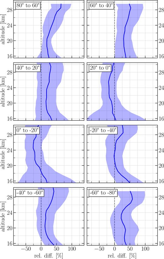
presented in Fig. 1a with the blue line. The estimate for the
tial gaps, which results in a less precise SO2 mass assessment
day when SO2 reached the stratosphere is marked with a red
(see Appendix C). Thus, the current choice provides a trade-
circle. The daily data coverage in percent, or the percentage
off between the spatial coverage and overall data availability.
of the self-defined grid that contains data that could be used
For the injection altitude estimation, MLS SO2 number
for the analysis, is depicted on the same panel with the gray
density profiles and tropopause altitude were used. Using the
line. Due to the large data gaps, this SO2 mass is a minimum
plume location from OMI/OMPS-NM and TROPOMI data
estimate for the SO2 injected during the eruption.
(see below), the profiles collocated with the plumes for April
The largest source of error for estimating the SO2 emission
and July 2018 were analyzed. Using this data, it was identi-
is probably the choice of the assumed SO2 profile because
fied that, on 6 April and the 27 July, the volcanic SO2 reached
the vertical distribution of the SO2 affects the air mass factor
the stratosphere. These days coincide with the information
used for the retrieval of the vertical column densities.
presented by Moussallam et al. (2019); Kloss et al. (2020);
Smithsonian Institution (2019). The profiles for the eruption
dates can be found in Appendix A1.
https://doi.org/10.5194/acp-21-14871-2021 Atmos. Chem. Phys., 21, 14871–14891, 202114876 E. Malinina et al.: Extinction coefficients after the 2018 Ambae eruption
Figure 1. The SO2 mass calculated for a threshold of 0.05 g m−2 from the combined OMI and OMPS-NM for the first Ambae eruption in
April (a) and from TROPOMI data for the July eruption (b).
3.1.2 TROPOMI data set the red circle, the day SO2 reached the stratosphere, accord-
ing to MLS data, is marked, while the data cover is depicted
The SO2 mass emitted during the eruption of Ambae in with a gray line. The SO2 mass increased to a maximum of
late July 2018 was estimated by analyzing SO2 total verti- 0.35 Tg on 27 July and declined, by 5 August, to magnitudes
cal columns from the TROPOMI instrument (see Sect. 2.6). of gigagram (hereafter Gg). The SO2 mass for a threshold
A grid with a resolution of 0.1◦ in both longitude and lati- of 0 g m−2 (not shown) exhibits a high SO2 background of
tude was defined from 10◦ N to 35◦ S and 150◦ E to 140◦ W. 0.1–0.15 Tg that quickly increases to a maximum of 0.51 Tg
We utilized sulfur dioxide total vertical columns, assuming on 27 July and decreases to 0.1 Tg on 5 August. The applica-
an SO2 profile represented by a 1 km thick box filled with tion of a threshold of 0 g m−2 seems to suggest an SO2 back-
SO2 and centered at 15 km altitude, in order to model con- ground of approximately 0.1–0.15 Tg that is not apparent in
ditions in an explosive eruption (Theys et al., 2017). Only Fig. 1 when using a more restrictive threshold. Focusing only
vertical column densities with values less than 1000 mol m−2 on the additional SO2 entry, i.e., the difference between the
were considered for the analysis. The data above this thresh- maximum SO2 and the background emission of 0.1–0.15 Tg,
old were excluded because they were considered unrealistic a total burden of approximately 0.35–0.4 Tg SO2 was emit-
and erroneous. Furthermore, a solar zenith angle less than ted, applying a threshold of 0 g m−2 . This result is compara-
70◦ (for the SO2 products that use an SO2 box profile) or ble to the maximal SO2 burden in Fig. 1.
a quality value greater than 0.5 (for the SO2 product that Furthermore, the calculated maximum of emitted SO2
uses TM5 model profile), respectively, was required (Theys mass strongly depends on the SO2 data product used. As
et al., 2020). The TM5 model is a global chemical transport mentioned in Sect. 3.1.1, the vertical SO2 distribution affects
model that provides a daily forecast of SO2 profiles (Theys the air mass factor that is used to retrieve the vertical column
et al., 2017). The total vertical column was multiplied by densities. Assuming a threshold of 0.05 g m−2 and an SO2
the SO2 molar mass to obtain the SO2 mass loading in the profile with the SO2 existing in a 1 km thick box at an altitude
units of g m−2 . Afterwards, similarly to Sect. 3.1.1, a thresh- of 15 km, as discussed above, results in the maximal SO2
old of 0.05 g m−2 was applied, and the SO2 mass in units of mass of 0.35 Tg. This value increases, respectively, to 0.5 Tg
grams for every grid segment was calculated. Since some or- and even to approximately 1.3 Tg by assuming, respectively,
bits overlap, 14 consecutive orbits covering a time span of a 1 km thick box at an altitude of 7 km and a profile from
approximately 24 h were bundled to a data set batch and av- the TM5 model. These results emphasize the importance of
eraged for each grid segment. Finally, the SO2 masses in all an accurate assumption for the vertical SO2 distribution (see
grid segments in the batch are summed up to obtain the total Appendix B).
SO2 burden.
The SO2 masses calculated for every batch and for the 3.2 OMPS-LP Ext retrieval algorithm
thresholds of 0.05 g m−2 during the Ambae eruption are pre-
sented in Fig. 1b. The date represents the date of the first or- As can be inferred from its name, initially OMPS was de-
bit in each batch that intersects with the area of interest. With signed to obtain ozone products, and in the instrument de-
Atmos. Chem. Phys., 21, 14871–14891, 2021 https://doi.org/10.5194/acp-21-14871-2021E. Malinina et al.: Extinction coefficients after the 2018 Ambae eruption 14877 sign, the UV-Vis parts of the spectrum were prioritized. As Malinina (2019). However, it was noticed that, by imple- the prism dispersion is nonlinear, the spectral resolution of menting the 0.002 km−1 threshold, some profiles with in- the measurements at the wavelength longer than 500 nm de- creased aerosol loading were incorrectly filtered for some grades exponentially, reaching about 30 nm at 1000 nm. This case studies. Thus, for an investigation of an isolated vol- results in the situation that the usual stratospheric aerosol canic eruption, a higher threshold is necessary to preserve all extinction wavelength 750 nm, used by, for example, SCIA- increased Ext values. The 0.1 km−1 value used in this study MACHY and OSIRIS (Rieger et al., 2018), is not suitable for is based on the experience with the 2019 Raikoke eruption use as OMPS-LP measurements around this wavelength are (Muser et al., 2020). For the user’s convenience, the products affected by the O2 -A absorption band. Thus, for the strato- with both cloud filters (0.002 and 0.1 km−1 ) are provided. spheric aerosol extinction retrieval, instead of 750 nm, we used the measurements at 869 nm (with a spectral resolution 3.3 Comparison of OMPS-LP and SAGE III/ISS of 22 nm) because the spectral interval from 830 to 900 nm is absorption free. The OMPS-LP Ext869 was originally retrieved to improve the Even though some aspects of our algorithm have been ozone product (Arosio et al., 2018); however, it can also be briefly described in Arosio et al. (2018) and Malinina (2019), used to evaluate the changes in stratospheric aerosol loading here we provide a consolidated summary. The OMPS V1.0.9 after volcanic eruptions and biomass burning events (Malin- aerosol extinction coefficient at 869 nm (Ext869 ) retrieval al- ina, 2019). Here, it should be noted that there are three other gorithm was adapted from the SCIAMACHY V1.4 algorithm OMPS aerosol extinction products; two of them are the of- (Rieger et al., 2018) and uses the same regularized iterative ficial NASA Ext675 products, i.e., V1.0 (Loughman et al., approach. However, here we used the first-order Tikhonov 2018) and V1.5 (Chen et al., 2018). Moreover, at the Univer- regularization with the parameter value of 50 to smooth spu- sity of Saskatchewan, as a part of the ozone retrieval, a tomo- rious oscillations in the level 1 V2.5 data. Using the infor- graphic Ext750 product was obtained (Bourassa et al., 2019). mation provided by NASA, the signal-to-noise ratio (SNR) All four Ext products were retrieved at different wavelengths is set to 500 for all tangent altitudes. and using different approaches. Thus, their comparison will In V1.0.9, Ext869 is retrieved on a regular 1 km grid from be not trivial and will contain uncertainties, e.g., associated 10.5 to 33.5 km, with the measurement at 34.5 km being with Ångström exponent calculations. used as the reference. Additionally, the effective Lambertian In order to evaluate the quality of our Ext869 , it was com- albedo is simultaneously retrieved using the Sun-normalized pared with the SAGE III/ISS solar occultation product. There spectrum at 34.5 km. The retrieval is done under the assump- are several advantages to this comparison. First, SAGE III is tion of stratospheric aerosols being spherical sulfate droplets an independent data set; thus, possible OMPS instrumental (75 % H2 SO4 and 25 % H2 O) with 0 % relative humidity issues (e.g., scattering angle dependency) will be revealed and unimodal lognormal particle size distribution (PSD). In by the comparison, which would not be the case when us- this distribution the median radius (rmed ) is equal to 0.08 µm ing other OMPS products. Second, SAGE III is an occulta- and σ = 1.6; the particle number density a priori profile was tion instrument, which means that its Ext profiles are rather chosen in accordance with the Extinction Coefficient for precise and independent of the aerosol PSD assumption, in STRatospheric Aerosol (ECSTRA) background climatology contrast to, for example, OSIRIS. The solar occultation mea- (Fussen and Bingen, 1999). We used the refractive indices surements are self-calibrating, and unlike limb instruments, from the OPAC (Optical Properties of Aerosols and Clouds) for the Ext retrieval, no assumptions on the aerosol particle database (Hess et al., 1998); for the selected wavelength, the size distribution are needed, thus making occultation mea- refractive index equals 1.425–1.38597 × 10⁻⁷ i. The strato- surements rather precise. spheric aerosol profile is defined from 10 to 46 km; below Another advantage of the comparison with SAGE III is and above, the number density profile is set to 0. After the the same measurement wavelength. Both OMPS-LP and retrieval, the Ext869 values higher than 0.1 km−1 are consid- SAGE III provide measurements at 869 nm, so no conversion ered to be cloud contaminated and, thus, are filtered. of the aerosol extinction to any other wavelength needs to be The threshold to reject clouds is selected empirically to done. Even though the spectral resolution of the instruments keep as much as possible of an event associated with in- at this wavelength is different (1.5 nm in SAGE III versus creased Ext and reject as many clouds as possible. However, 30 nm in OMPS-LP), it does not influence the aerosol ex- the trade-off between these two factors is determined by the tinction coefficient strongly because the wavelength interval potential application of the data set. For instance, for appli- from 830 to 900 nm is absorption free. cations where it is more important to remove as many clouds For the comparison, individual profiles from 7 June 2017 as possible and single high aerosol peaks are not of a great until 31 August 2019 were used. The profiles were collo- value, a rather conservative value of 0.002 km−1 is recom- cated using the following criteria: the difference between the mended. This value is based on the results from Bourassa profile’s coordinates should be less than 2.5◦ in latitude, 10◦ et al. (2010), where the Ext750 after the Kasatochi eruption in longitude, and 24 h in time. The minimal time difference did not exceed 0.001 km−1 . This threshold was used in, e.g., between profiles was 01:47:37 h, while the maximum dif- https://doi.org/10.5194/acp-21-14871-2021 Atmos. Chem. Phys., 21, 14871–14891, 2021
14878                                               E. Malinina et al.: Extinction coefficients after the 2018 Ambae eruption

                                                                    example, at about 28 km altitude, the differences reach up to
                                                                    60 % in these latitude bins.
                                                                       Generally, the above-described differences are similar
                                                                    to the relative differences between SCIAMACHY V1.4,
                                                                    OSIRIS v5.07, and SAGE II v7 (Rieger et al., 2018; Ma-
                                                                    linina, 2019). Additionally, Chen et al. (2020) showed that
                                                                    the differences seen between the OMPS Ext675 V1.5 and
                                                                    SAGE III product have the same shape and order of mag-
                                                                    nitude. Rieger et al. (2018) studied precisely the reasons for
                                                                    the observed differences. Since the OMPS V1.0.9 algorithm
                                                                    is very similar to the SCIAMACHY V1.4 algorithm used
                                                                    in that study, and since the OMPS and SCIAMACHY have
                                                                    very similar geometries, the same explanations, as given by
                                                                    Rieger et al. (2018), are appropriate. According to this study,
                                                                    the most important sources of errors in limb retrievals arise
                                                                    from the uncertainly assumed aerosol loading at the reference
                                                                    tangent altitude and the unknown aerosol particle size distri-
                                                                    bution parameters. The latter factor mostly affects the high
                                                                    latitudes where the viewing geometries are close to forward
                                                                    and backward scattering.
                                                                       Based on our comparison and the results from the other
                                                                    limb-occultation instrument studies, it can be concluded that
                                                                    our OMPS V1.0.9 Ext869 is of sufficient quality to be used
                                                                    for scientific purposes.

                                                                    3.4   OMPS-LP aerosol extinction climatology

                                                                    In order to study the aerosol extinction coefficient evolution
                                                                    after a volcanic eruption, the OMPS V1.0.9 product has to be
                                                                    averaged in some fashion. We have created two level 3 prod-
                                                                    ucts, which are monthly and 10 d averaged Ext869 . Both prod-
                                                                    ucts were binned onto a regular geographical grid with 2.5◦
Figure 2. Mean relative difference in Ext869 between                latitude and 5◦ longitude steps. Since the retrieved product
OMPS-LP and SAGE III/ISS calculated as 200 × (OMPS-                 is provided on the regular 1 km grid, no vertical averaging is
SAGE)/(OMPS+SAGE). The shaded areas show ± 1 standard               needed.
deviation.                                                             An example of zonal monthly mean Ext869 averaged in 30◦
                                                                    latitude bins for the whole OMPS operation period is pre-
                                                                    sented in Fig. 3. In this figure, the volcanic eruptions and a
                                                                    relevant biomass burning event are shown with gray triangles
ference is 22:07:38 h. Overall, there are 19 264 collocated         with numbers. The information on the volcanic eruptions is
measurements used for this comparison. For SAGE III data,           presented in Table 1. We show only Ext869 within 60◦ in both
similarly to OMPS, the aerosol extinction values higher than        hemispheres because, as it was pointed out in Sect. 3.3, the
0.1 km−1 were filtered out. Additionally, the SAGE III Ext869       aerosol extinctions above these latitudes are associated with
values were excluded if the uncertainty provided by NASA            larger uncertainties. Furthermore, the main scope of this pa-
is higher than 50 %. We did not filter negative Ext869 because      per is to study the tropical Ambae eruptions; thus, we do not
this would bias the comparison (see Damadeo et al. (2013)           focus our attention on aerosol loading in the high latitudes.
for details).                                                          Analysis of Fig. 3 shows that there is a certain increase
    The mean relative differences between OMPS and                  in Ext869 at the very beginning of OMPS operation in the
SAGE III Ext869 are presented in Fig. 2 in 20◦ latitude bins.       Northern Hemisphere in the bin between 60◦ and 30◦ . This
For most of the altitudes in all latitude bins, the relative dif-   is associated with the eruption of Nabro (13◦ N) in the mid-
ference is within 25 %. In the tropical and midlatitudes, the       dle of 2011. Additionally, one can see an increase in Ext869
only exceptions are the altitudes below 18 km, where, despite       some time after the eruptions in Table 1 and from the Cana-
filtering, the influence of clouds is still present. The largest    dian wildfires of 2017 (number 5 in Fig. 3 and Table 1). The
differences are observed in high latitudes (40◦ to 80◦ in both      degree of the enhancement, and the time lag between the
hemispheres), in particular at the altitudes above 24 km. For       eruptions seen in the latitude bands, are dependent on the

Atmos. Chem. Phys., 21, 14871–14891, 2021                                           https://doi.org/10.5194/acp-21-14871-2021
E. Malinina et al.: Extinction coefficients after the 2018 Ambae eruption 14879
Table 1. Volcanic eruptions and biomass burning events shown in Fig. 3.
No. Event Date of eruption Latitude Longitude
1 Copahue 23 Dec 2012 −37.51 −71.1
2 Kelut 13 Feb 2014 −7.55 112
3 Sangeang Api 30 May 2014 −8.2 119.07
4 Calbuco 22 Apr 2015 −41.19 −72.37
5 Canadian wildfires Jul–Aug 2017 51.64 −121.3
6 Ambae 6 Apr 2018 −15.4 167.84
6a 27 Jul 2018
7 Raikoke 22 Jun 2019 48.3 153.4
8 Ulawun 26 Jul 2019 −5.05 151.33
Figure 3. Monthly mean aerosol extinction coefficient (Ext869 ) distribution as a function of time and altitude. The values were obtained
by binning and zonally averaging OMPS-LP monthly level 3 Ext869 . The white lines show 0.00005 km−1 Ext869 level. The triangles with
numbers represent volcanic eruptions and biomass burning events (see Table 1).
volcano’s location and the eruption strength. Usually, for the is seen as yearly reoccurring lighter colored stripes, in both
tropical eruptions, an increase in stratospheric aerosol load- Tropics and midlatitudes is related to two factors. First, there
ing is seen globally because the aerosols and precursors are are some yearly changes in stratospheric aerosol loading
transported with the Brewer–Dobson circulation (BDC) to (Hitchman et al., 1994; Bingen et al., 2004). Second, for
both hemispheres. Also, in the Tropics, the BDC is respon- the limb-viewing instruments, an important factor is the sea-
sible for the tape recorder effect or the delayed increase in sonality in solar scattering angle, which leads to artifacts of
Ext869 with height (Vernier et al., 2011). For example, in the retrieval predominately in the extratropical regions (see,
Fig. 3a and b, the tape recorder effect is seen for the Ke- e.g., Rieger et al., 2018). Additionally, for the tropical re-
lut, Sangeang Api, Calbuco, and Ambae eruptions, as well as gion, there is a periodic signal above 25 km altitude associ-
for the Canadian wildfires. For the eruptions in the midlati- ated with the quasi-biennial oscillation (QBO). It can be seen
tudes, the increase usually stays in the hemisphere where it in the thin white line, which represents the 0.00005 km−1
occurred (e.g., Oman et al., 2006; von Savigny et al., 2015; Ext869 level. However, as with the other altitudes, this Ext869
Toohey et al., 2019; Malinina, 2019). level is somewhat affected by the annual variation in addi-
Another readily identifiable feature in Fig. 3 is the peri- tion to the QBO. Here, it is important to mention that, dur-
odical increase in Ext in all latitude bins. There are several ing the OMPS operation period, two QBO disruptions were
drivers causing this pattern. The annual seasonality, which reported, namely in 2015–2016 (Newman et al., 2016) and
https://doi.org/10.5194/acp-21-14871-2021 Atmos. Chem. Phys., 21, 14871–14891, 202114880 E. Malinina et al.: Extinction coefficients after the 2018 Ambae eruption
2019–2020 (Kang and Chun, 2021). These disruptions might there until late June. In June, the increase in Ext869 starts
also mask the changes in the high-altitude extinctions. Gen- to spread to the south, reaching 35–45◦ S in July 2018. At
erally, the influence of the QBO on stratospheric aerosols 20.5 km, the increase after the first SO2 release is rather neg-
is well known and was previously reported by, e.g., Vernier ligible. Nevertheless, there is still an area with the increased
et al. (2011); Hommel et al. (2015); Brinkhoff et al. (2015); aerosol loading below 20◦ S from the beginning of May.
von Savigny et al. (2015); Malinina et al. (2018). In late July 2018, during the fourth phase of the erup-
One should also mention the increase in the extinction at tion, Ambae injected another portion of ash and SO2 . Al-
approximately 16.5–17 km in Fig. 3a and b and at around most at the same time, Ext869 increases at 18.5 km directly
13.5–15 km in Fig. 3c and d. These are the residual clouds at the source. In about 2 weeks, the volcanic plume starts
which were not filtered by our threshold. Though we show to spread both northward and southward and is located be-
the data in Fig. 3 above the average tropopause height for tween the Equator and 35◦ S in early September, reaching
the bin, some overshooting convective clouds still could be 45◦ N in November–December 2018. The southern border
present and influence an average Ext. Here we want to high- of the plume at 18 km is harder to identify because it mixes
light that we are aware of disadvantages of our fixed cloud with the aerosol from the previous SO2 release. However, an
filtering threshold, which can also be considered quite high. increased aerosol loading is observed to the south of 35◦ S
As we state above in Sect. 3.2, our previous threshold was too in September and intensifies further with the time. By mid-
low and was filtering out parts of volcanic and forest fires October 2018, at 18.5 km, the plume shows a clear reduction
plumes. Furthermore, any fixed threshold would either fil- around the Equator and continues to weaken with time. At
ter out some high-extinction events or leave some fractions 20.5 km, the plume appears in mid-September 2018 at around
of cloud in. However, the other commonly used cloud filter- 10◦ S and spreads northwards and southwards from that mo-
ing approach exploiting altitude derivative of spectral ratio ment on, reaching its maximum in November. It is located in
also suffers from poor discrimination under certain condi- between 30◦ S and 35◦ N in mid-December 2018. Again, at
tions (Chen et al., 2016; Rieger et al., 2019). the southern border of the plume, there is an area of increased
Ext869 , which is related to both eruptions.
4 Ambae eruption 4.1.2 Ambae eruption modeled by ECHAM
4.1 Aerosol extinction coefficient evolution
The Ambae experiment setup used the estimated SO2 emis-
As it was highlighted in the introduction, Ambae was one sions from Sect. 3.1 and the injection altitudes from MLS
of the largest eruptions of the last decade but has not been data (see Appendix A). As pointed out, the result of the cal-
a focus of scientific or public interest. The eruptive period, culated SO2 mass from OMI/OMPS data for the April erup-
which lasted over a year, had two explosive phases when SO2 tion provides only a minimum estimate because the analy-
was injected into the stratosphere (the exact information on sis suffered from large data gaps. In accordance with Kloss
SO2 mass estimation can be found in Sect. 3.1). The first et al. (2020), an SO2 mass of 0.12 Tg was chosen as a realis-
emission was smaller, and the perturbation in Ext869 did not tic assumption for the April eruption in the simulation. Thus,
reach altitudes above 21 km (see Fig. 3a and b). The second we injected 0.12 Tg SO2 at altitudes of 82 to 102 hPa on the
emission was considerably larger; it perturbed Ext869 up to 6 April for 4 h and 0.36 Tg SO2 at altitudes between 74 and
23.5 km in the Tropics and up to 22 km in the extratropical 90 hPa on 27 July for 24 h, starting at 18:00 UTC (universal
regions. However, to better evaluate the plume evolution, we coordinated time). During the review process, the extension
will further analyze 10 d averaged Ext869 . of the self-defined grid for the TROPOMI analysis was re-
duced to exclude SO2 artifacts at the borders, which resulted
4.1.1 Ambae eruption as seen by OMPS-LP in a slight decrease in the estimated SO2 mass from 0.36 to
0.35 Tg. The ECHAM simulations were carried out with the
The evolution with time and altitude of the 10 d averaged former value, but we do not expect a significant impact due to
zonal mean Ext869 at 18.5 and 20.5 km is presented in Fig. 4a that difference. The long eruption phase was chosen to take
and b. Foremost, it should be noted that the increase in the observed series of eruptions into account. To slow down
Ext869 in February–May 2018 in the latitudes above 25◦ N at the oxidation of SO2 due to the limited availability of OH
18.5 km and above 7◦ N at 20.5 km is related to the disappear- in a volcanic cloud (Mills et al., 2017), the concentration of
ing plume from the Canadian wildfires of 2017. Already in OH was limited in the first days after the eruption, i.e., day 1
the first week after the eruption a small increase in Ext869 is to 10 was limited to 40 % and day 10 to 20 to 60 % of the
seen around the Ambae location; however, this increase can- prescribed OH. The sea surface temperature (SST) is set to a
not be uniquely attributed to the Ambae eruption and can be climatological value (Hurrell et al., 2008).
caused by the transport of the aerosol from preceding events. In order to be consistent with OMPS-LP measurements,
The more significant increase is observed in early May 2018. the output of ECHAM was interpolated to the same verti-
At the time, the plume is located around 10–25◦ S and stays cal grid as provided by OMPS-LP. ECHAM provides Ext at
Atmos. Chem. Phys., 21, 14871–14891, 2021 https://doi.org/10.5194/acp-21-14871-2021E. Malinina et al.: Extinction coefficients after the 2018 Ambae eruption 14881
Figure 4. The evolution of the aerosol extinction coefficient (Ext869 ) at 18.5 and 20.5 km altitude after the Ambae eruptions of 2018. In
panels (a) and (b), Ext869 was retrieved from OMPS-LP measurements; for panels (c) and (d), Ext869 was modeled by MAECHAM5-HAM.
Both data sets were averaged over 10 d periods.
550 and 825 nm; thus, for consistency in the comparison, the pear. In late December, the Ext increase is seen from 30◦ N
simulated Ext was recalculated to 869 nm, and afterwards, to 45◦ S.
the 10 d averages were calculated. The simulated distribution
of Ext869 with time and latitude at 18.5 and 20.5 km is pre- 4.1.3 Discussion
sented in Fig. 4c and d. In these panels, it is seen that, at
18.5 km, the aerosol extinction coefficient starts to increase In order to evaluate the consistency of the results from OMPS
almost right after the first eruption and reaches its peak in and ECHAM, the panels in Fig. 4 need to be compared. It is
May. The majority of the volcanic aerosol stays in the Trop- obvious that the model and the observations are very close to
ics between 30◦ S and the Equator. A small amount of aerosol each other, in particular at 18.5 km. The plume from the first
is dispersed meridionally right after the eruption. After the eruption appears and intensifies at the same time at 18.5 km;
second eruption, at the end of July, the first aerosol is formed however, in the model it is weaker, and it reaches 20.5 km
right after the eruption, with Ext increasing slowly until it about a month later. This is most likely related to the fact that,
reaches the maximum in September. Most aerosols are lo- in the model, neither the anthropogenic nor biomass burning
cated to the south of 10◦ N. In the last days of September, the sources are taken into account.
plume is still very well pronounced, and it starts to spread The Ambae plume from the July eruption looks even more
meridionally, mostly southwards. By beginning of October, similar in the model results and measurements. Not only does
Ext increases also in the Northern Hemisphere at 20◦ N; this the plume appear at the same time, at 18.5 km, and is lo-
increase spreads with the time to 40◦ in the late December. cated at the same latitudes, but also both model and mea-
The plume starts to weaken at the beginning of November. surements show a wave-shape of the plume. The curvature
At 20.5 km, the plume from the first eruption appears in in both plumes appears in mid-September; however, in the
late June. The plume at this altitude is quite weak and does OMPS-LP data, the plume is bending stronger to the north.
not extend much over the latitudes. Basically, it is a small It should also be noted that the ECHAM simulations show a
area in between the Equator and 10◦ S. The increase in Ext more intensive and longer living plume at this altitude. Addi-
associated with the second eruption appears at 20.5 km in tionally, in the OMPS-LP data, in the second part of October,
very late August; by the middle of September, the plume in- the aerosols move north- and southward evenly, while in the
tensifies and starts to expand meridionally. It reaches its max- ECHAM data, the plume is instead transported to the south.
imum by November, when the increase is seen from 10◦ N to In ECHAM data at 20.5 km, the July plume appears about
40◦ S. From that moment, the plume starts to slowly disap- 2–3 weeks earlier than in the OMPS measurements. Though
the intensity of the modeled plume at this altitude is slightly
https://doi.org/10.5194/acp-21-14871-2021 Atmos. Chem. Phys., 21, 14871–14891, 202114882 E. Malinina et al.: Extinction coefficients after the 2018 Ambae eruption
weaker, the absolute differences are smaller than at 18.5 km.
However, the horizontal distribution of the modeled plume is
less consistent with the measurements. While the plume in
ECHAM data stays, with the time, in the same latitude band
mostly in the Southern Hemisphere, in the OMPS data, it has
a C-shape around the Equator.
It should be highlighted that, even though there are some
differences between the modeled and measured Ext, the
consistency is quite remarkable. There are key main fac-
tors which contributed to this particular agreement between
OMPS and ECHAM, namely, rather precise SO2 mass and
height estimation, as well as nudging of meteorological data.
Consequently, it is seen that the second plume, whose emis-
sion was estimated from TROPOMI data, was modeled more
accurately. At the same time, our internal studies showed that
the ECHAM SO2 sensitivity plays a key role in the lifetime
and distribution of the plume (see Fig. S1 in the Supplement).
It is a well-known feature of ECHAM that the meridional
transport is too strong, causing a relatively short lifetime of
sulfate (e.g., Niemeier et al., 2009), especially compared to
results of other models (e.g., Marshall et al., 2018). There-
fore, the nudging of the meteorological data provided a re-
alistic transport pattern resulting in good agreement with
OMPS-LP measurements. However, the nudging database, Figure 5. Evolution of zonal mean aerosol extinction coefficient
the ERA5 reanalysis, has not only observational but also a (Ext869 ) in the Tropics (20◦ S–20◦ N), with altitude and time after
strong model component as well. Thus, small differences the Ambae eruptions of 2018. In panel (a), the data from OMPS-LP
with observations are rather possible, especially in the strato- are presented, and in panel (b) the simulation with MAECHAM5-
sphere. Additionally, the stratospheric aerosol layer is close HAM is plotted. Both data sets were averaged over a 10 d periods.
to the ozone layer at 24 km. ECHAM uses the prescribed
ozone and OH values which do not change due to the pres-
tion given by Eq. (1), as suggested by Hansen et al. (2005)
ence of volcanic aerosol.
the following:
Another way to assess the degree of consistency between
the model and the measurements is to analyze the vertical RF ≈ −25 · τ550 , (1)
distribution of Ext with the time (see Fig. 5). Since most
of the plume stayed in the tropical region, for Fig. 5, the where τ550 is the stratospheric aerosol optical depth at
OMPS (Fig. 5a) and ECHAM (Fig. 5b) Ext were averaged 550 nm. Although originally proposed for the globally av-
between 20◦ S and 10◦ N. In this figure, it is again obvious eraged model data, Eq. (1) was successfully used for the RF
that, in the model, the perturbation from the volcano reached assessment from the measurement results (see, e.g., Solomon
the same altitudes. Additionally, it is observed that the plume et al., 2011; von Savigny et al., 2015). As the focus of our
was weaker for the April eruption. However, consistency for study is on the additional RF after the tropical Ambae erup-
the second eruption is again striking. The plume has the same tions, we do not consider global averages but limit the com-
overall shape and is located at the same time coordinates. A parison to 20◦ S–20◦ N region.
disagreement is seen, however, around the 19.5 km altitude in To apply Eq. (1) to the OMPS-LP data, we deter-
November, where OMPS-LP data show an increased extinc- mined τ550(869) by integrating the Ext869 from instantaneous
tion not present in ECHAM simulations. Also, Kloss et al. tropopause height to 33.5 km and then converting the result to
(2020) report maximum extinction in the 18–19 km layer in 550 nm wavelength by using an Ångström exponent of 2.47,
November when analyzing OMPS-LP data. The reasons for which is appropriate for the particle size distribution used in
the observed disagreements are still under investigation. the Ext869 retrieval (see Sect. 3.2). The tropopause height val-
ues were obtained for each single OMPS-LP measurement by
4.2 Radiative forcing using corresponding ECMWF-ERA5 temperature profiles.
The World Meteorological Organization (WMO) definition
In order to assess the RF from the Ambae eruption, we ana- of the tropopause, based on the temperature lapse rate, was
lyzed the top-of-the-atmosphere ECHAM RF output and the implemented (WMO, 1957), and the tropopause height cal-
top-of-the-atmosphere RF calculated from OMPS-LP mea- culation algorithm follows the one from Appendix A (1) of
surements. For the latter, we use the empirical approxima- Maddox and Mullendore (2018). Afterwards, the τ550(869)
Atmos. Chem. Phys., 21, 14871–14891, 2021 https://doi.org/10.5194/acp-21-14871-2021You can also read