Capital income breeding in wild boar: a comparison between two sexes - Nature
←
→
Page content transcription
If your browser does not render page correctly, please read the page content below
www.nature.com/scientificreports
OPEN Capital‑income breeding in wild
boar: a comparison between two
sexes
Rudy Brogi1*, Roberta Chirichella1, Francesca Brivio1, Enrico Merli2, Elisa Bottero1 &
Marco Apollonio1
Organisms differ in the strategy adopted to fuel reproduction by using resources either previously
acquired and stored in body reserves (capital breeding) or, conversely, acquired during their
reproductive activity (income breeding). The choice of one or the other strategy is related to several
internal and external factors which are counteractive in wild boar. Based on a large dataset of culled
wild boar, we investigated individual body weight variability throughout the period of 1st September–
31st January, which included the main part of the mating season, among different sex and age classes
to determine their position along the capital-income breeding continuum. Though food resources
were abundant during the rut, adult males lost body weight suggesting they adopted a predominantly
capital breeding strategy, likely owing to the high intra-sexual competition entailed by the peculiar
mating system of the species. On the contrary, subadult males seemed to behave as income breeders,
likely enhancing the reproductive flexibility of wild boar populations. During the rut, females stored
reserves, thus suggesting that they substantially relied on them to cover future reproductive costs.
The life history of an animal is comprised of sets of trade-offs among growth, survival, and reproduction that
organisms face during their life1. A major aspect of life history diversity among animal species is that the resources
allocated to reproduction are obtained either from stored reserves within the body or the current intake, resulting
in the division between capital and income breeders (e.g.,2,3). This concept is of utmost importance in theoretical
evolutionary ecology as it influences both the body condition-reproductive success relationship and the time lag
of organisms-environmental resources linkage3, but it can also be profitably applied to conservation and manage-
ment as it affects a species’ sensitivity to environmental c hanges3,4. Furthermore, given the wide exploitation of
ungulates in hunting and their growing involvement in wildlife-human conflicts, their life histories are raising
a strong interest among researchers.
Stephens and c olleagues3 reported that the degree of capital and income breeding of organisms is related to
a variety of ecological, morphological, and physiological factors. In particular, high food availability during the
breeding season typically promotes income breeding strategies2, while temporal mismatches between resource
supply and reproductive demand promote capital b reeding5. Larger body size can facilitate capital breeding on
account of a lower relative cost for reserve transportation and a higher metabolism efficiency3. The mating system
and, specifically, the degree of polygyny may act as a further push-factor in positioning male ungulates along
the capital-income c ontinuum6. Indeed, higher levels of intra-sexual male competition for mating opportuni-
ties are likely to enhance the reproductive demands of polygynous males and, concomitantly, their tendency to
adopt feeding r eduction7,8 and s uppression9,10 during the rut, inevitably forcing them to rely on a stored capital
of reserves. Moreover, in order to maximize their lifetime reproductive success, individuals can occupy differ-
ent positions along the capital-income breeding continuum throughout their life c ycles5. Indeed, adult male
ungulates typically show high body weight loss during the rut (i.e., high reliance on stored reserves) compared
to younger males which, conversely, give priority to growth. As a consequence, young males show a limited or
null body weight loss (for a review, see Mysterud et al.11), although they can still be fully or partially involved
in reproduction12,13. When evaluating life history strategies, it is therefore essential to first characterise sex and
age classes, as groups of individuals at different stages of the growth-reproduction trade-off are likely to adopt
different strategies for the acquisition of resources to invest in reproduction.
One of the major constraints for studies on capital-income breeding lies in the difficulty to objectively cir-
cumscribe the time period over which the reproductive costs should be m easured3. As female investment into
reproduction usually includes a variety of activities linked to a single reproductive event (for mammals: mating,
1
Department of Veterinary Medicine, University of Sassari, via Vienna 2, 07100 Sassari, Italy. 2Agriculture and
Wildlife Service, Emilia-Romagna Region, via Garibaldi 50, 29122 Piacenza, Italy. *email: r.brogi@studenti.uniss.it
Scientific Reports | (2021) 11:4579 | https://doi.org/10.1038/s41598-021-84035-w 1
Vol.:(0123456789)www.nature.com/scientificreports/
foetuses growth, giving birth, and lactation), studies on females are particularly concerned with the difficulties
in circumscribing the period of such reproductive costs. Conversely, since most male ungulates have no further
reproductive cost after c onception11, their reproductive effort is entirely included in the rutting season. Neverthe-
less, finding an objective way to circumscribe this period on a local level entails several practical complications.
Previous studies on male ungulate life histories arbitrarily delimited the r ut14, obtained it from other studies15,
or roughly derived it from field behavioural o bservations16.
As a rare example of highly polygynous species17, exhibiting similar early-life growth rates in both sexes
(e.g.,18) and a short generation time compared to other ungulates (e.g.,19,20), wild boar (Sus scrofa) is a particularly
interesting species for studying life history strategies. The position of wild boar along the capital-income breeding
continuum has previously only been determined for females and was found to be different according to the area
and the study19,21,22, with litter size being the only measure of reproductive effort considered. Conversely, males’
reliance on the stored capital or the available resource income for reproduction has never been investigated,
though this sex presents a unique combination of contrasting factors pushing simultaneously towards the two
opposite strategies. On the one hand, the mating period occurs when food resources are relatively abundant. This
should prevent the need of previously stored energy and facilitate income breeding. Oak (Quercus spp.), chestnut
(Castanea sativa), and beech (Fagus sylvatica) seed production, which accounts for most of European wild boar’s
diet (at least in natural and semi-natural situations in which agricultural crops are scarce and supplementary
feeding is not provided23,24), is typically concentrated in late autumn, when mating usually occurs25. On the other
hand, wild boar morphology and reproductive biology should push males to adopt capital breeding, by reducing
costs associated with this strategy and accounting for feeding suppression, respectively. As a matter of fact, large
size and a thermally efficient body shape (sensu A llen26) should enhance wild boar metabolism efficiency, thus
reducing costs of capital storing, transportation, and maintenance. The relatively high degree of polygyny of this
species17 entails high competition among males for mating opportunities. This may be expected to increase both
the need and the potential reproductive value of relying on stored reserves and thus promote capital b reeding6.
27 28
In addition, the gregarious habits of females and the high litter size make male reproductive effort even more
beneficial in terms of potential number of descendants, thus exacerbating intra-male competition.
Age can also be expected to heavily determine individual strategies to fuel reproduction, as younger wild boar
still need to allocate part of the resources to growth. Consequently, they have lower body reserves to invest29.
As mentioned above, it becomes essential to discuss individuals’ reproductive reliance on stored reserves in the
context of their growth stages, typically represented by age classes. Nevertheless, the available growth curves
on wild boar are provided by studies limited by the use of either a small sample size30,31, or descriptive statistics
alone18, or both32,33.
When relatively high, hunting pressure can also play a role in shaping wild boar reproductive strategies, as
an unbalanced removal of adult individuals can influence the first reproduction of both subadult males34 and
females19. If the harvest is adult male-biased (not the case of our study a rea35), hunting can also cause a shortage
of adult males and, therefore, lower the levels of sexual competition36, thus potentially reducing the reproduc-
tive effort and ultimately the need of capital breeding. Nevertheless, an opposite effect (i.e., increased male
reproductive costs) was described by Mysterud et al.14 in female-skewed moose (Alces alces) populations, likely
because males had to enhance their displacements in order to take advantage of the higher number of available
female groups.
Based on a large dataset of culled wild boar, we first modelled male and female body growth curves and identi-
fied age classes in order to properly compare breeding strategies among homogeneous groups of individuals. To
independently determine the period over which male reproductive effort is sustained, we assessed female oestrus
distribution throughout the year and used it as a proxy of the rutting season. We then compared body weight
variability throughout autumn–winter in different sex and age classes in order to evaluate potential changes in
male weight with respect to other classes owing to their reproductive effort. In so doing, we aimed to ascertain
their position along the capital-income breeding continuum.
Results
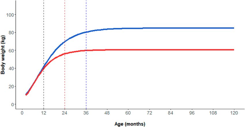
Sex and age class identification. Gompertz growth models’ estimated parameters, summarised in Sup-
plementary Table S1, were all statistically significant. Sexual size dimorphism appeared around 1 year of age.
Males had to reach 3 years of age to exceed 90% of their asymptotical weight (85 kg), while the age for females
was 2 years (female asymptotical weight = 61 kg, Fig. 1). On this basis, the following sex and age classes were
identified: male and female piglets (individuals younger than 1 year), subadult males (males older than 1 year
but younger than 3 years), subadult females (females older than 1 year but younger than 2 years), adult males
(males older than 3 years), and adult females (females older than 2 years). Sample distribution among sex and
age classes is reported in Supplementary Table S2.
Rutting season identification. The intra-annual distribution of conception dates started in October,
peaked in January and lasted until April, with most events concentrated in the period December-March (Fig. 2).
The portion of conception events occurring during the sampling period (153 days starting from 1st September)
was 59.68 ± 5.00% (mean ± SE) of the total.
Seasonal variability of individual body weight in different classes. All selected best models (iden-
tified following the minimum Akaike’s Information Criterion, AIC, see Methods for more details) significantly
explained body weight variability (p-values of all included predictor are reported in Supplementary Tab. S3).
Adult males’ best model included sampling day, individual age, previous winter rain precipitation, and spring
temperature as predictor variables ( R2adj = 0.100). Throughout the sampling period, adult males showed a non-
Scientific Reports | (2021) 11:4579 | https://doi.org/10.1038/s41598-021-84035-w 2
Vol:.(1234567890)www.nature.com/scientificreports/
Figure 1. Body weight variation of males (blue line) and females (red line) at growing ages. Values were
predicted by the Gompertz growth models separately for males and females (see the text for more details).
Vertical dashed lines represent the limits between piglets-subadults (both sexes, black line), subadult-adult
females (red line), subadult-adult males (blue line).
Figure 2. Conception event smoothed distribution throughout the year assessed from individual age of piglets
and subadult individuals, culling date, and gestation period (see the text for more details). Upper and lower
thin lines represent the distribution of mean + SE and mean − SE, respectively. Date is expressed as days from
1st September and equivalent to the sampling day. The dashed line represents the end of the sampling period
(153 days, from 1st September to 31st January).
linear pattern of body weight variability, with a slight increase during the first part of the sampling period (last-
ing approximately 50 days) and a subsequent steady loss. Predicted weights ranged from a maximum of about
91 kg (around the 50th day of the sampling period) to 82 kg (at the end of the sampling period, Fig. 3a), thus
showing a weight loss of 9.89%. As they grew older, adult males showed only a slight, constant weight gain.
Adult male weights increased with increasing spring average temperature, until reaching a maximum peak with
an average temperature of 8.0 °C, then slightly decreased above this optimal value, and finally stabilised above
9.5 °C. A slightly positive effect of previous winter rain precipitation was detected (see Supplementary Fig. S1).
The best model explaining adult female body weight variability included sampling day, individual age, and
previous year chestnut productivity as predictor variables (R2adj = 0.214). Adult females gained body weight with
a steady pattern throughout the sampling period, starting with an average weight of 55 kg and reaching up to
68 kg at the end of the period (Fig. 3b), with a total gain of 23.64% of the initial weight. In accordance with the
Scientific Reports | (2021) 11:4579 | https://doi.org/10.1038/s41598-021-84035-w 3
Vol.:(0123456789)www.nature.com/scientificreports/
Figure 3. Body weight variation of adult males (a), adult females (b), subadult males (c), subadult females (d),
male piglets (e), and female piglets (f) throughout the sampling period. The first sampling day corresponds to
1st September. Values were predicted by the best models separately for each class. Grey-shaded areas represent
the estimated standard errors. The predictions are given according to the mean of all other covariates in the
models.
results of the Gompertz body growth model, adult females showed substantially stable weights at growing ages.
Though statistically significant, previous year chestnut productivity had a positive but biologically negligible
effect on adult female body weight (Supplementary Fig. S2).
The best model predicting subadult male body weight variability included the following set of predictor vari-
ables: sampling day, individual age, previous year chestnut productivity, previous winter, spring, and summer
average temperatures ( R2adj = 0.238). Their body weight showed only small variations throughout the sampling
period (predicted values: 55–61 kg), with an initial slight increase lasting about 50 days, followed by a horizontal
pattern lasting for the rest of the season (Fig. 3c). Individual age had a clear, positive effect on the predicted body
weight, while previous year chestnut productivity accounted for slightly higher body weight. Finally, the average
Scientific Reports | (2021) 11:4579 | https://doi.org/10.1038/s41598-021-84035-w 4
Vol:.(1234567890)www.nature.com/scientificreports/
temperature of the summer and spring months preceding the hunting season negatively affected subadult male
body weight, while that of the previous winter months did not show any relevant effect (Supplementary Fig. S3).
Subadult female body weight variability was explained by the best model including sampling day, individual
age, previous summer average temperature, previous winter rain precipitation, and current autumn rain pre-
cipitation as predictor variables ( R2adj = 0.233). Females of this age class showed a steady increase of their body
weight throughout the sampling period, a result which is similar to that of adult females, though with wider
confidence intervals (Fig. 3d). Moreover, the relation with age was positive. As with subadult males, the best
model predicted a substantial negative relation between body weight and previous summer average temperature.
Subadult females reached their maximum body weight with mean values of rain precipitation during the previ-
ous winter (around 4 mm/day), while higher values of current autumn rain (above 5.0 mm/day) accounted for
heavier body weights (Supplementary Fig. S4).
The best model explaining the variability of male piglet body weight included the predictors: sampling day,
individual age, current year global productivity index, mean rain precipitation of previous summer, and aver-
age temperature of previous spring (R2adj = 0.370). In this class, body weight increased with a steady pattern
throughout the sampling period until the 110th sampling day and slightly decreased during last 40 days of
hunting (Fig. 3e). Individual age had a positive effect on the response variable, with older male piglets being
constantly heavier than younger ones. The relation between male piglet body weight and current year global
productivity index was linear and positive, whereas other predictor variables had a significant but biologically
negligible effect (Supplementary Fig. S5).
As for female piglets, the best model included sampling day, individual age, and previous year Turkey oak
(Quercus cerris) productivity as predictor variables ( R2adj = 0.331). Their predicted body weight increased through-
out the sampling period, with a pattern essentially identical to that of male piglets (Fig. 3f). Likewise, a positive
effect of individual age was assessed. Finally, female piglet body weight was higher when previous year Turkey
oak productivity was around 0.4 Mg/ha (Supplementary Fig. S6).
Discussion
We investigated wild boar capital-income breeding strategies by using a large dataset of culled individuals. We
objectively characterised age classes and quantitatively assessed the timing of the rut with a large sample of
conception dates and a comprehensive account of uncertainty. Our results suggest that adult males relied on a
stored capital of reserves to cope with their reproductive requirements, although weight gains of other classes
confirmed the expectation that food resources were particularly abundant during the rut.
Our sex and age classification on the basis of growth stages is consistent with that used in previous studies
with regards to piglets of both sexes and females in g eneral19,25,36. On the contrary, the subdivision between
subadult and adult males was placed at 3 years, unlike other studies (2 years in33,34,36). As males were clearly still
growing between 2 and 3 years of age, they could not afford a full investment in reproduction, despite being
already sexually mature37, which is the typical condition of subadults. In this respect, we would argue that our
classification better generalised male growth stages. This enabled us to properly compare body weight variation
patterns and breeding strategies among homogenous groups of individuals.
Only adult males showed an absolute weight loss during the sampling period (1st September–31st January),
whereas all other classes gained body weight, though with different extents and patterns (Fig. 3). Food resources
were particularly abundant during that time of the year, as confirmed by weight gains of other classes as well as by
data referring to wild boar spatial behaviour within the same area38. Since hunting disturbance is known to have
a minimal impact on wild boar b ehaviour39,40 and the rich-food habitats (forest) are also the safest refuges from
35
hunting risk in our study area , we can exclude the possibility that hunting affected the weight loss observed in
adult males. Reproductive efforts were more likely to be the main cause of this negative trend, as supported by
the temporal match between the start of adult male body weight decrease (around the 50th sampling day) and
the start of the conception event distribution. We may directly estimate a relative loss of about 9.89% of the pre-
reproductive adult male body weight (50th sampling day), though the total weight loss related to reproduction
was likely much higher. Indeed, our sampling period was constrained by hunting season limits and covered only
a part of the rutting season, including 59.68 ± 5.00% of all conception events (Fig. 2). If the relation between body
weight loss and conception event distribution had remained the same as it was observed during the sampling
period, we can estimate that adult males would have lost 16.57 ± 1.39% of their pre-reproductive body weight
by the end of the rut. Adult male wild boar relative weight loss estimated by our analysis can be compared with
that of male Alpine chamois (Rupicapra rupicapra rupicapra, 17–19% in Mason et al.16 and 16.0% in Apollonio
et al.6) and male red deer (Cervus elaphus, 19.5% in Apollonio et al.6), which are usually considered capital
breeders6,14. Accordingly, our results position adult male wild boar towards the capital end of the capital-income
breeding continuum.
Both the reproduction effort itself and feeding reduction or suppression during the rutting season possibly
accounted for the reproduction-induced weight loss of adult males. Though information on male wild boar
reproductive behaviour is still lacking, during the rut they are thought to roam widely in search for groups of
receptive females, actively competing to monopolise and finally mate with them41,42. This behavioural pattern is
likely to enhance the energetic expenditure of males during the rut. Even though hunting pressure may partially
weaken the direct competition to monopolise female groups by unbalancing the population structure toward
females36, a female-skewed population has been shown to increase male reproductive cost in other species (e.g.,
in moose14). This is likely due to a higher energy expenditure in spatial movements, as each male would have the
opportunity to mate with several scattered female groups. Nevertheless, in such a food-rich season, the massive
weight loss observed can hardly be explained by energy expenditure alone. However, the almost total feeding sup-
pression which characterises a number of male polygynous ungulates (see M iquelle9 for moose; Apollonio and Di
Scientific Reports | (2021) 11:4579 | https://doi.org/10.1038/s41598-021-84035-w 5
Vol.:(0123456789)www.nature.com/scientificreports/
ittorio10 for fallow deer, Dama dama) would be unaffordable for wild boar, given the long-lasting rut. Indeed, it
V
was never detected in studies involving the analysis of wild boar stomach c ontent23,43. We can therefore presume
that adult male wild boar may adopt milder forms of feeding reduction during the rut, similarly to male Alpine
ibex (Capra ibex)7 and Alpine chamois8. This explanation is supported by the decrease of the insulin-like growth
factor 1 concentrations (IGF-I, whose secretion is linked with energy supply) observed in males during autumn
and winter by Treyer et al.43. This may have also contributed to weaken the effect of food abundance during the
rut in determining the adoption of an income breeding strategy, by preventing individuals to fully exploit it.
Similarly to adult males, subadult males increased their body weight during the first part of the sampling
period but then showed substantially stable values, with an almost flat slope (Fig. 3c). As they are still growing,
subadult males may not have considerable stored reserves available for reproduction. The temporary 2–3 month
growth break observed may indicate that subadult males took part in reproduction (as previously suggested by
Šprem et al.34), though investing only resources from the current intake and thus behaving as income breeders.
Since income breeding can only support a small reproductive investment and a direct competition with adults
would be totally ineffective for them44, we can argue that subadult males relied on alternative mating tactics
to achieve at least some p aternities12,13. Wild boar social organisation may have also contributed to the missed
weight gain observed in this class. Indeed, during the rut adult males display agonistic behaviours against sub-
adult males joining females g roups27, potentially moving them away from food-rich areas, which are typically
occupied by females. Thus, we can argue that subadult males’ reproductive contribution is inversely dependent
on the availability of adult males in the population. This may therefore potentially reduce the negative effect of
a male-biased culling on the reproductive outcomes.
Both adult and subadult females gained body weight almost steadily during the whole sampling period
(Fig. 3b,d). However, this result did not allow us to directly determine their position along the capital-income
breeding continuum. Indeed, female reproductive investment can be considered negligible during the mating
season, then becoming substantial during the subsequent phases of foetuses formation, birth, and weaning, which
essentially occupy the rest of the year. While subadult females were still growing and therefore may have allocated
the resources acquired during autumn–winter to body growth, adult females have already completed their body
development and reasonably invested the resources stored during this period in the subsequent reproduction
phases. This suggests that adult females substantially relied on reserves stored in autumn–winter to cover future
reproductive costs and, thus, adopted a capital breeding strategy.
We used a long-lasting dataset sampled during 14 consecutive hunting seasons but limited to 5 months per
year. This prevented us from properly evaluating females’ reproductive reliance on stored reserves and observ-
ing the last portion of the rutting season. However, we managed to predict the total reproductive cost carried
by adult males by means of a quantitative and independent assessment of rut timing. Our large sample size
provided a robust insight into wild boar life history at a population level, which would have been unfeasible
with longitudinal studies as they are typically limited to few monitored individuals (e.g.,12,45 ). Nevertheless,
further well-designed longitudinal studies may be extremely useful to evaluate the heterogeneity of wild boar
life history on an individual level.
In conclusion, we demonstrated that adult male wild boar adopted a predominantly capital breeding strategy,
while subadult males likely behaved as income breeders and enhanced the reproductive flexibility of the popula-
tions. Though we were not able to directly assess females’ strategy, we detected a strong resource storage during
the mast period, which is likely to be invested in the subsequent reproduction effort. Being capital breeders
generally less sensitive to environmental v ariability3,4, we can argue that wild boar reproductive outcomes will
be highly resilient to ecological perturbations.
Materials and methods
Study area. Our study was conducted in the Alpe di Catenaia mountainous area (Northern Apennines,
Italy, 43° 48′ N, 11° 49′ E, Supplementary Fig. S7) which covers a total surface of 13,400 ha and includes a pro-
tected area (Oasi Alpe di Catenaia) of 2,700 ha. Altitude ranges from 330 to 1,414 m above the sea level. The
temperate-continental climate shows marked seasonal variations, with hot and dry summers (mean temperature
of 18.7 °C and daily precipitation of 1.73 mm) and cold and rainy winters (mean temperature of 1.2 °C and daily
precipitation of 3.55 mm). Snowfalls occur only occasionally between October and April. The area is mainly
covered with mixed deciduous woods (67% of the total surface), with Turkey oak, beech, and chestnut as the
most abundant tree species, while conifer woods (7%), agricultural crops (16%), and mixed open-shrubs areas
(10%) cover the rest of the surface. Wild boar unselective drive hunts (i.e. targeting all social classes) involved
25–50 hunters and were performed in the surroundings of the protected area three times a week from Septem-
ber–October to January (on average of 58.3 hunting days per year). Hunting pressure was high and relatively
constant over the years, with an average of 6.4 wild boar/km2 harvested every year35.
Data collection. We collected data on 8,763 wild boar of all age and sex classes culled within our study
area from 1st September to 31st January in the period 2002–2016, for a total of 14 consecutive hunting seasons.
Undressed body weight and culling date were recorded for each wild boar. Since female reproductive traits were
not fully available for measurements, we could not subtract foetus weight from pregnant female body weight,
thus potentially overestimating their body condition. Nevertheless, foetus weight (calculated on a subsample of
415 pregnant females with measurable reproductive traits) accounted for a negligible portion of mother total
body weight (on average 0.51 ± 0.95%, mean ± SD). On the basis of their tooth eruption and abrasion46, all wild
boar were assigned to one of the following age intervals: < 3 months, 3–4 months, 5–6 months, 7–9 months,
10–12 months, 13–14 months, 15–16 months, 17–18 months, 19–20 months, 20–22 months, 22–24 months,
24–36 months, 3–4 years, 5–7 years, 8–10 years or > 10 years. Given the intrinsic characteristics of the tooth-
Scientific Reports | (2021) 11:4579 | https://doi.org/10.1038/s41598-021-84035-w 6
Vol:.(1234567890)www.nature.com/scientificreports/
based aging method, we are aware that precision decreased as age increased. Notwithstanding, this was the only
feasible approach to age a large number of culled individuals.
Yearly seed productivity of beech, chestnut, and Turkey oak was acquired from an online database reporting
local data collected in our study a rea47. Weather data were recorded daily in a weather station located inside our
study area (43° 42′ N, 11° 55′ E) and kindly provided by the Regional Hydrological Service of Tuscany.
Ethical declarations. Data collection did not involve any alive animal. All wild boar included in analysis
were culled according to Italian national and regional hunting laws.
Data analysis. Sex and age class identification. As we aimed to assess patterns of body growth of both
sexes during different age stages, we distinguished culled individuals into males and females, thus creating 2
sub-datasets out of our original dataset (males, n = 4398, and females, n = 4365). We then assigned individual
ages as the median of the age interval identified by means of tooth analysis. For each sub-dataset, body growth
was then described by fitting weight to age with the Gompertz growth equation45,48,49 through a 3-parameter
nonlinear model:
−cx
W = a ∗ e−be
in which W is body weight at age x, a is the asymptotic body weight, e is the exponential constant, b is the dis-
placement on the x-axis, and c is growth rate. We estimated a, b and c by means of the SSgompertz function of the
stats package in R 3.2.250. Finally, we used the growth curves obtained to identify 2 breakpoints: (i) age of sexual
size dimorphism appearing and (ii) age of body weight exceeding 90% of its asymptotic value (sex-specific),
rounding them on a yearly basis to correctly distinguish cohorts. Depending on their individual age, male and
female wild boar were separately grouped into 3 age classes: piglets (below first breakpoint), subadults (above
the first and below the second breakpoint) and adults (above the second breakpoint).
Rutting season identification. In order to identify the rutting season for the studied population, we estimated
the temporal distribution of conception events. Individual conception dates were estimated from the age of
culled piglet and subadult wild boar, culling date and gestation period, following the formula:
CoD = CuD − IA − GP
with CoD being the conception date, CuD the culling date, IA the individual age expressed in days of the culled
wild boar, and GP an average gestation period of 118 days (obtained as the mean between a gestation period of
115 days reported by H enry51 and of 121 days reported by V ericad52). IA was estimated as the median of the age
interval identified. Only wild boar aged 2 years or younger were included in analyses, as their age interval width
was ≤ 3 months, for a total of 6604 individuals. In order to take into account both sources of uncertainty (gesta-
tion period and ageing process), we smoothened the number of conception events occurring per date by means
of the loess function of the stats package in R. We used a 41-day span width, i.e., the average standard error of
conception date attribution, which was calculated as 1/1.96 of the sum of the mean age interval width (74 days)
and the 6-day difference between two conception periods. Finally, we quantified the portion of conception events
which occurred during our sampling period.
Seasonal variability of individual body weight in different classes. In order to evaluate the variability of indi-
vidual body weight throughout the sampling period and its relation with reproduction efforts, we divided our
dataset into 6 sub-datasets corresponding to sex and age classes previously identified by means of body growth
models (adult males, n = 752, adult females, n = 1376, subadult males, n = 1629, subadult females, n = 1318, male
piglets, n = 2017, and female piglets, n = 1671). Individual body weight was modelled by means of Generalised
Additive Models (GAMs) with a Gaussian distribution, which were implemented by means of the mgcv package
in R, separately for each sub-dataset. Sampling day was standardised as the number of days from 1st September
and used as predictor to observe the variability of individual body weight throughout the sampling period.
In order to enhance the models’ robustness, we also included individual age, previous and current year forest
productivities, and weather variables as predictors. Individual age, expressed in months, was calculated as the
median of the age interval identified by means of the tooth analysis and used to take into account the residual
age-related source of variation in individual body weight. Current and previous year productivity of Turkey
oak, beech, and chestnut, expressed as Mg/ha, were measured on a yearly basis and included in the models to
consider inter-annual variability of food resource availability and its potential effect on individual body weight.
Moreover, we included a global forest productivity index, which was calculated as the sum of the relative produc-
tivity of all three species, which were in turn obtained as the ratio of the productivity of a certain tree species in
a given year over the mean productivity of the same species during the entire study period38. Finally, to account
for the potential indirect effect of weather on individual body weight of wild boar, we included the seasonal
average of temperature and rain precipitation in the models. Since all individuals were culled during the hunting
season of year x, seasonal temperature and seasonal rain precipitation were calculated on a yearly basis with the
following rule: weather variables were averaged from December of year x-1 to February of year x in winter, from
March to May of year x in spring, from June to August of year x in summer, and from September to November
of year x in autumn. Values of the 8 weather variables (average temperature and average daily rain precipitation
for each of the four seasons) were then assigned to each individual according to the hunting season of culling.
For each sub-dataset discretely, predictors were screened for collinearity (Pearson correlation matrix, rp) and
multicollinearity (Variance Inflation Factor), with thresholds set to r p = ± 0.7 and VIF = 3, respectively53. Among
Scientific Reports | (2021) 11:4579 | https://doi.org/10.1038/s41598-021-84035-w 7
Vol.:(0123456789)www.nature.com/scientificreports/
the different sub-datasets, the most recurring groups of variables affected by collinearity included forest pro-
ductivities of the same year, especially the chestnut-Turkey oak and beech-global index productivity pairs, and
mean temperature and daily precipitation of the same season, particularly spring and autumn. To select the best
candidate predictors among the collinear variables, we screened them by means of a machine learning method,
the random forest calculation (random.Forest package), which ranked all predictor variables on the basis of their
potential to explain body weight v ariability54. We dropped the worst predictor variable of each collinearity con-
dition until no variable affected by multicollinearity remained.
The final step of analysis consisted of a model selection process for each sub-dataset. We built a full GAM
which included all the predictor variables selected in the previous step, with the effect of all variables modelled
as a natural cubic spline function. Subsequently, we used the dredge function of the MuMln package to run a
set of models with all possible combinations of the full model predictor variables. The best models were then
identified following the minimum AIC and the most parsimonious (in terms of number of predictor variables
included) were selected in case of pairs and groups of models with ΔAIC < 255. We performed a validation of the
models selected by visually inspecting their residuals to check for homoscedasticity, normality of errors, and
independence53.
Data availability
The dataset analysed during the current study is available from the corresponding author on reasonable request.
Received: 10 November 2020; Accepted: 25 January 2021
References
1. Bednekoff, P. A. Life histories and Predation risk. In Encyclopedia of Animal Behavior 283–287 (Elsevier, Amsterdam, 2010).
2. Jönsson, K. I. Capital and income breeding as alternative tactics of resource use in reproduction. Oikos 78, 57 (1997).
3. Stephens, P. A., Boyd, I. L., McNamara, J. M. & Houston, A. I. Capital breeding and income breeding: their meaning, measurement,
and worth. Ecology 90, 2057–2067 (2009).
4. Kerby, J. & Post, E. Capital and income breeding traits differentiate trophic match–mismatch dynamics in large herbivores. Philos.
Trans. R. Soc. B 368, 20120484 (2013).
5. Williams, C. T. et al. Seasonal reproductive tactics: annual timing and the capital-to-income breeder continuum. Philos. Trans. R.
Soc. B 372, 20160250 (2017).
6. Apollonio, M. et al. Capital-income breeding in male ungulates: Causes and consequences of strategy differences among species.
Front. Ecol. Evol. 8, 308 (2020).
7. Brivio, F., Grignolio, S. & Apollonio, M. To feed or not to feed? Testing different hypotheses on rut-induced hypophagia in a
mountain ungulate. Ethology 116, 406–415 (2010).
8. Corlatti, L. & Bassano, B. Contrasting alternative hypotheses to explain rut-induced hypophagia in territorial male chamois. Ethol-
ogy 120, 32–41 (2014).
9. Miquelle, D. G. Why don’t bull moose eat during the rut?. Behav. Ecol. Sociobiol. 27, 145–151 (1990).
10. Apollonio, M. & Di Vittorio, I. Feeding and reproductive behaviour in fallow bucks (Dama dama). Naturwissenschaften 91, 579–584
(2004).
11. Mysterud, A., Langvatn, R. & Stenseth, N. C. Patterns of reproductive effort in male ungulates. J. Zool. 264, 209–215 (2004).
12. Coltman, D. W., Festa-Bianchet, M., Jorgenson, J. T. & Strobeck, C. Age-dependent sexual selection in bighorn rams. Proc. R. Soc.
Lond. B 269, 165–172 (2002).
13. Apollonio, M., Brivio, F., Rossi, I., Bassano, B. & Grignolio, S. Consequences of snowy winters on male mating strategies and
reproduction in a mountain ungulate. Behav. Process. 98, 44–50 (2013).
14. Mysterud, A., Solberg, E. J. & Yoccoz, N. G. Ageing and reproductive effort in male moose under variable levels of intrasexual
competition. J. Anim. Ecol. 74, 742–754 (2005).
15. Garel, M. et al. Sex-specific growth in Alpine Chamois. J. Mammal. 90, 954–960 (2009).
16. Mason, T. H. E. et al. Contrasting life histories in neighbouring populations of a large mammal. PLoS ONE 6, e28002 (2011).
17. Dardaillon, M. Le sanglier et le milieu Camarguais: Dynamique Coadaptative. (1984).
18. Spitz, F., Valet, G. & Lehr Brisbin, I. Variation in body mass of wild boars from southern France. J. Mammal. 79, 251–259 (1998).
19. Servanty, S., Gaillard, J., Toïgo, C., Brandt, S. & Baubet, E. Pulsed resources and climate-induced variation in the reproductive
traits of wild boar under high hunting pressure. J. Anim. Ecol. 78, 1278–1290 (2009).
20. Gamelon, M. et al. Fluctuating food resources influence developmental plasticity in wild boar. Biol. Lett. 9, 20130419 (2013).
21. Frauendorf, M., Gethöffer, F., Siebert, U. & Keuling, O. The influence of environmental and physiological factors on the litter size
of wild boar (Sus scrofa) in an agriculture dominated area in Germany. Sci. Total Environ. 541, 877–882 (2016).
22. Gamelon, M. et al. Reproductive allocation in pulsed-resource environments: a comparative study in two populations of wild boar.
Oecologia 183, 1065–1076 (2017).
23. Massei, G., Genov, P. V. & Staines, B. W. Diet, food availability and reproduction of wild boar in a Mediterranean coastal area. Acta
Theriol. (Warsz.) 41, 307–320 (1996).
24. Schley, L. & Roper, T. J. Diet of wild boar Sus scrofa in Western Europe, with particular reference to consumption of agricultural
crops. Mamm. Rev. 33, 43–56 (2003).
25. Canu, A. et al. Reproductive phenology and conception synchrony in a natural wild boar population. Hystrix 26, 77–84 (2015).
26. Allen, J. A. The influence of physical conditions in the genesis of species. Radic. Rev. 1, 108–140 (1877).
27. Fernández-Llario, P., Carranza, J. & De Trucios, S. H. Social organization of the wild boar (Sus scrofa) in Doñana National Park.
Misc. Zool. 19, 9–18 (1996).
28. Bywater, K. A., Apollonio, M., Cappai, N. & Stephens, P. A. Litter size and latitude in a large mammal: the wild boar Sus scrofa.
Mamm. Rev. 40, 212–220 (2010).
29. Merta, D., Mocała, P., Pomykacz, M. & Frąckowiak, W. Autumn-winter diet and fat reserves of wild boars (Sus scrofa) inhabiting
forest and forest-farmland environment in south-western Poland. J. Vertebr. Biol. 63, 95–102 (2014).
30. Ježek, M., Štípek, K., Kušta, T., Červený, J. & Vícha, J. Reproductive and morphometric characteristics of wild boar (Sus scrofa) in
the Czech Republic. J. For. Sci. 57, 285–292 (2011).
31. Markina, F. A., Cortezo, R. G. & Gómez, C.S.-R. Physical development of wild boar in the Cantabric Mountains, Álava, Nothern
Spain. Galemys Bol. Inf Soc. Esp. Para Conserv. Estud. Los Mamíferos 16, 25–34 (2004).
32. Gallo Orsi, U., Macchi, E., Perrone, A. & Durio, P. Biometric data and growth rates of a wild boar population living in the Italian
Alps. J. Mt. Ecol. 3, 60–63 (1995).
Scientific Reports | (2021) 11:4579 | https://doi.org/10.1038/s41598-021-84035-w 8
Vol:.(1234567890)www.nature.com/scientificreports/
33. Pedone, P., Mattioli, S. & Mattioli, L. Body size and growth patterns in wild boars of Tuscany, Central Italy. J. Mt. Ecol. 3, 66–68
(1995).
34. Šprem, N. et al. Morphometrical analysis of reproduction traits for the wild boar (Sus scrofa L.) in Croatia. Agric. Conspec. Sci. 76,
263–265 (2011).
35. Merli, E., Grignolio, S., Marcon, A. & Apollonio, M. Wild boar under fire: the effect of spatial behaviour, habitat use and social
class on hunting mortality. J. Zool. 303, 155–164 (2017).
36. Poteaux, C. et al. Socio-genetic structure and mating system of a wild boar population. J. Zool. 278, 116–125 (2009).
37. Mauget, R. & Boissin, J. Seasonal changes in testis weight and testosterone concentration in the European wild boar (Sus scrofa
L.). Anim. Reprod. Sci. 13, 67–74 (1987).
38. Bisi, F. et al. Climate, tree masting and spatial behaviour in wild boar (Sus scrofa L.): Insight from a long-term study. Ann. For. Sci.
75, 46 (2018).
39. Keuling, O., Stier, N. & Roth, M. How does hunting influence activity and spatial usage in wild boar Sus scrofa L.?. Eur. J. Wildl.
Res. 54, 729–737 (2008).
40. Brivio, F. et al. An analysis of intrinsic and extrinsic factors affecting the activity of a nocturnal species: the wild boar. Mamm. Biol.
84, 73–81 (2017).
41. Singer, F. J., Otto, D. K., Tipton, A. R. & Hable, C. P. Home ranges, movements, and habitat use of European wild boar in Tennessee.
J. Wildl. Manag. 45, 343–353 (1981).
42. Dardaillon, M. Wild boar social groupings and their seasonal changes in the Camargue, southern France. Z. Für Säugetierkd. 53,
22–30 (1988).
43. Treyer, D. et al. Influence of sex, age and season on body weight, energy intake and endocrine parameter in wild living wild boars
in southern Germany. Eur. J. Wildl. Res. 58, 373–378 (2012).
44. Festa-Bianchet, M. The cost of trying: weak interspecific correlations among life-history components in male ungulates. Can. J.
Zool. 90, 1072–1085 (2012).
45. Knott, K. K., Barboza, P. S. & Bowyer, R. T. Growth in arctic ungulates: postnatal development and organ maturation in Rangifer
tarandus and Ovibos moschatus. J. Mammal. 86, 121–130 (2005).
46. Briedermann, L. Wild boars. Deutscher Landwirtschaftsverlag (1990).
47. Chianucci, F. et al. Multi-temporal dataset of stand and canopy structural data in temperate and Mediterranean coppice forests.
Ann. For. Sci. 76, 80 (2019).
48. Zullinger, E. M., Ricklefs, R. E., Redford, K. H. & Mace, G. M. Fitting sigmoidal equations to mammalian growth curves. J. Mam-
mal. 65, 607–636 (1984).
49. Sand, H., Cederlund, G. & Danell, K. Geographical and latitudinal variation in growth patterns and adult body size of Swedish
moose (Alces alces). Oecologia 102, 433–442 (1995).
50. R Development Core Team. R: A Language and Environment for Statistical Computing (R Foundation for Statistical Computing,
Vienna, 2015).
51. Henry, V. G. Length of estrous cycle and gestation in European Wild Hogs. J. Wildl. Manag. 32, 406 (1968).
52. Vericad Corominas, J. R. Estimación de la edad fetal y períodos de concepción y parto del jabalí (Sus scrofa L.) en los Pirineos
occidentales. (1981).
53. Zuur, A., Ieno, E. N., Walker, N., Saveliev, A. A. & Smith, G. M. Mixed Effects Models and Extensions in Ecology with R (Springer
Science & Business Media, Berlin, 2009).
54. Breiman, L. Random forests. Mach. Learn. 45, 5–32 (2001).
55. Symonds, M. R. & Moussalli, A. A brief guide to model selection, multimodel inference and model averaging in behavioural ecol-
ogy using Akaike’s information criterion. Behav. Ecol. Sociobiol. 65, 13–21 (2011).
Acknowledgements
We are grateful to the hunters who collaborated with us and to all researchers, students, and volunteers who
contributed in collecting data, especially E. Bertolotto, N. Cappai, E. Donaggio and D. Battocchio. We also wish
to thank the Regional Hydrological Service of Tuscany for providing meteorological data. C. Polli kindly edited
the English version of this manuscript. The research was financially and logistically supported by the Provincial
Administration of Arezzo and the Italian Ministry of Education, University and Research (PRIN 2010-2011,
20108 TZKHC).
Author contributions
M.A. originally formulated the idea. R.C. and E.B. conducted fieldwork. R.B., F.B. and E.M. collaborated in imag-
ing and performing analysis. R.B. wrote the original draft of the manuscript. M.A., F.B., R.C. and E.M. provided
editorial advice. M.A. provided materials tools and contributed to funding acquisition.
Competing interests
The authors declare no competing interests.
Additional information
Supplementary Information The online version contains supplementary material available at https://doi.
org/10.1038/s41598-021-84035-w.
Correspondence and requests for materials should be addressed to R.B.
Reprints and permissions information is available at www.nature.com/reprints.
Publisher’s note Springer Nature remains neutral with regard to jurisdictional claims in published maps and
institutional affiliations.
Scientific Reports | (2021) 11:4579 | https://doi.org/10.1038/s41598-021-84035-w 9
Vol.:(0123456789)www.nature.com/scientificreports/
Open Access This article is licensed under a Creative Commons Attribution 4.0 International
License, which permits use, sharing, adaptation, distribution and reproduction in any medium or
format, as long as you give appropriate credit to the original author(s) and the source, provide a link to the
Creative Commons licence, and indicate if changes were made. The images or other third party material in this
article are included in the article’s Creative Commons licence, unless indicated otherwise in a credit line to the
material. If material is not included in the article’s Creative Commons licence and your intended use is not
permitted by statutory regulation or exceeds the permitted use, you will need to obtain permission directly from
the copyright holder. To view a copy of this licence, visit http://creativecommons.org/licenses/by/4.0/.
© The Author(s) 2021
Scientific Reports | (2021) 11:4579 | https://doi.org/10.1038/s41598-021-84035-w 10
Vol:.(1234567890)You can also read